READ THESE TERMS AND CONDITIONS CAREFULLY BEFORE USING THIS WEBSITE.
https://nrc-publications.canada.ca/eng/copyright
Vous avez des questions? Nous pouvons vous aider. Pour communiquer directement avec un auteur, consultez la
première page de la revue dans laquelle son article a été publié afin de trouver ses coordonnées. Si vous n’arrivez pas à les repérer, communiquez avec nous à PublicationsArchive-ArchivesPublications@nrc-cnrc.gc.ca.
Questions? Contact the NRC Publications Archive team at
PublicationsArchive-ArchivesPublications@nrc-cnrc.gc.ca. If you wish to email the authors directly, please see the first page of the publication for their contact information.
NRC Publications Archive
Archives des publications du CNRC
This publication could be one of several versions: author’s original, accepted manuscript or the publisher’s version. / La version de cette publication peut être l’une des suivantes : la version prépublication de l’auteur, la version acceptée du manuscrit ou la version de l’éditeur.
Access and use of this website and the material on it are subject to the Terms and Conditions set forth at Commissioning twin houses for assessing the performance of energy conserving technologies
Swinton, M. C.; Moussa, H.; Marchand, R. G.
https://publications-cnrc.canada.ca/fra/droits
L’accès à ce site Web et l’utilisation de son contenu sont assujettis aux conditions présentées dans le site LISEZ CES CONDITIONS ATTENTIVEMENT AVANT D’UTILISER CE SITE WEB.
NRC Publications Record / Notice d'Archives des publications de CNRC: https://nrc-publications.canada.ca/eng/view/object/?id=da3c9800-f6f9-4937-aa5b-84d40b7e6774 https://publications-cnrc.canada.ca/fra/voir/objet/?id=da3c9800-f6f9-4937-aa5b-84d40b7e6774
Canadian
Centre
Centre
canadien
des
for Housing Technology
technologies résidentielles
Commissioning twin houses for assessing the performance of energy conserving technologies
Swinton, M.C.; Moussa, H.; Marchand, R.G.
NRCC-44995
A version of this document is published in / Une version de ce document se trouve dans: Proceedings for Performance of Exterior Envelopes of Whole Buildings VIII: Integration of Building
The Canadian Centre for Housing Technology (CCHT)
Built in 1998, the Canadian Centre for Housing Technology (CCHT) is jointly operated by the National Research Council, Natural Resources Canada, and Canada Mortgage and Housing Corporation. CCHT's mission is to accelerate the development of new technologies and their acceptance in the marketplace.
The Canadian Centre for Housing Technology features twin research houses to evaluate the whole-house performance of new technologies in side-by-side testing. The twin houses offer an intensively monitored real-world environment with simulated occupancy to assess the performance of the residential energy technologies in secure premises. This facility was designed to provide a stepping-stone for manufacturers and developers to test innovative technologies prior to full field trials in occupied houses.
As well, CCHT has an information centre, the InfoCentre, which features a showroom, high-tech meeting room, and the CMHC award winning FlexHouse™ design, shown at CCHT as a demo home. The InfoCentre also features functioning state-of-the art equipment, and demo solar photovoltaic panels. There are over 50 meetings and tours at CCHT annually, with presentations and visits occurring with national and international visitors on a regular basis.
Commissioning Twin Houses for Assessing the Performance
of Energy Conserving Technologies
Michael C. Swinton*1, member of ASHRAE, P.E. , Hussein Moussa2, Roger G. Marchand3
ABSTRACT
In 1998, twin houses were built at the Canadian Centre for Housing Technology in Ottawa to assess the energy performance of new and innovative energy efficient materials and components for houses. The two research houses are identical energy efficient houses typical of tract-built models available on the local housing market. They also feature identical simulated occupancies based on home-automation technologies and are monitored for energy performance and thermal comfort. The simulated occupancy controls turn on and off major appliances, lighting and equipment. The houses were commissioned in the winter and spring of 1999, and benchmarked in the next heating season. This paper records the energy features of the houses and
commissioning results. With the benefit of detailed monitoring of energy systems in both houses, many of the anomalies in component operation and controls were found and fixed. These anomalies could easily go undetected in regular houses.
Keywords: residential, energy measurement, consumption, space heating, water heating, energy analysis, commissioning.
1 Michael C. Swinton is a senior research officer, Institute for Research in Construction, National Research Council Canada, and is Research
Manager at the Canadian Centre for Housing Technology.
2 Hussein Moussa formerly a technical officer, Institute for Research in Construct ion, National Research Council Canada, now an applications
engineer with Alfieri-Proctor Associates, Boston.
Commissioning Twin Houses for Assessing the Performance
of Energy Conserving Technologies
Michael C. Swinton*1, member of ASHRAE, P.E. , Hussein Moussa2, Roger G. Marchand3
ABSTRACT
In 1998, twin houses were built at the Canadian Centre for Housing Technology in Ottawa to assess the energy performance of new and innovative energy efficient materials and components for houses. The two research houses are identical energy efficient houses typical of tract-built models available on the local housing market. They also feature identical simulated occupancies based on home-automation technologies and are monitored for energy performance and thermal comfort. The simulated occupancy controls turn on and off major appliances, lighting and equipment. The houses were commissioned in the winter and spring of 1999, and benchmarked in the next heating season. This paper records the energy features of the houses and
commissioning results. With the benefit of detailed monitoring of energy systems in both houses, many of the anomalies in component operation and controls were found and fixed. These anomalies could easily go undetected in regular houses.
Keywords: residential, energy measurement, consumption, space heating, water heating, energy analysis, commissioning.
1
Michael C. Swinton is a senior research officer, Institute for Research in Construction, National Research Council Canada, and is Research Manager at the Canadian Centre for Housing Technology.
2
Hussein Moussa formerly a technical officer, Institute for Research in Construction, National Research Council Canada, now an applications engineer with Alfieri-Proctor Associates, Boston.
3
INTRODUCTION
The concept of side-by-side testing of whole house performance in not new. Four side-by-side houses were built in the suburbs of Ottawa in 1977 [Quirouette 1978] and monitored extensively for a number of years [Brown 1980]. The energy efficiency measures being assessed in that project were initially built into the houses. The project assessed the total impact of design packages involving many different energy upgrades in each house. This is in contrast to the current facility, which was designed to assess individual technologies separately. As well, the original houses were initially unoccupied and later occupied by different families – both situations being problematic for realistic assessments of the technology packages. Later, two pairs of identical UK and Swedish prefab houses were built in the UK, [Rayment et al, 1993, 1997]. These were initially identical and featured automated controls based on laboratory control techniques to regulate energy usage inside the houses. Although these houses were successful in assessing individual energy conserving measures, these houses were not typical of North American style houses (e.g. only 84m2 livable area and no basement), and operated in the moderate UK climate.
In 1998, twin houses were built at the Canadian Centre for Housing Technology to assess the energy performance of new and innovative energy efficient materials and components for houses in the Canadian context. The two research houses – the reference house and the test house – were built to a design submitted by a local builder for the project. The houses are typical in construction, appearance and layout of tract-built houses available on the local housing market. They are identical, and are built to the R-2000 standard - Canada’s benchmark for energy efficient house design. They are approximately 210 m2 liveable area, and feature a full basement and a two-car garage.
The research houses also feature standard sets of major appliances typically found in North American homes. A system based on home automation technology simulates human activity by operating appliances, lighting and other equipment according to an identical schedule in both houses. The simulated occupancy system is also used to monitor energy performance.
This paper describes the commissioning process of the twin research houses, highlighting the main elements that were found to be different from a thermal performance point of view, and needing correction. Performance benchmark characteristics were developed against which energy saving devices could be rated in side-by-side comparisons.
Description of the Test and Reference house
The two houses were built side-by-side in the fall of 1998. The same trades built the houses by stages in sequence from one house to the other; e.g. footings were poured in one house then the next, then basement walls etc. The houses were never more than two weeks apart in the
construction process at any point in time. Construction was stopped at the pre-drywall stage for 2 ½ weeks to allow the installation of over 250 sensors in each house. As well 21 electric, gas and water flow meters were installed. The houses were completed in January 1999. We refer to one house as the “reference house”, which is intended to remain unchanged through the various experiments at the facility. The second house is referred to as the “test house”, in which
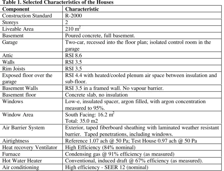
different energy-efficient technologies are assessed. The technologies are always installed in such a way that the test house can be returned to the original configuration which we refer to as the “benchmark configuration”. Table 1 lists selected characteristics of the two houses, and Table 2 lists the meters installed.
The reference house is a typical 2-storey wood-frame house, with 210m2 of liveable area, set on a cast-in-place concrete basement, with style and finish representative of current houses available on the local housing market. The house is built to meet the R-2000 Standard with a package that includes tight, well insulated assemblies, low-e argon filled sealed glazing units. It has a high efficiency sealed combustion condensing gas furnace, a power-vented conventional hot water heater and a heat recovery ventilator. The furnace, water heater and gas fireplace are all vented through the wall, eliminating the need for chimneys. The house has an airtightness characteristic of 1.07 ach @ 50 Pa – well below the R-2000 requirement of 1.5 ach @ 50 Pa. The monitoring and control room is located in an isolated room built in the garage with special conduits leading to each floor, to run wiring. The conduits were sealed on completion or the wiring. The test house was notionaly identical to the reference house, but this had to be verified through the commissioning process. For example, its airtightness characteristics was 0.97 ach @ 50 Pa – 10% lower than the reference house. We needed to determine how this and a whole host of other factors would affect the overall thermal performance of each of the houses.
After a first round of commissioning and benchmarking, the test house was modified to
incorporate several heating systems by incorporating a split plenum with dampers, in the forced air distribution system. The benchmark was unchanged by this adaptation, as verified in
subsequent weeks of benchmarking. A network of piping and valves was also developed to accommodate several water heaters. The houses are shown in Photo 1.
Data Collection
Four sets of data were collected during the test period. These were:
1. The main data set of approximately 250 sensors (mostly temperatures and RH) collected to keep track of operating conditions inside and out. Data was saved on an hourly basis, and a selected set was saved every 5 minutes.
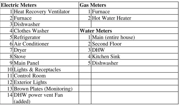
2. Utility meter readings (2 gas meters, 14 electric meters and 5 water flow meters – data stored hourly – see Table 2).
3. Weather data from a weather station situated about 350 m north and west of the houses (hourly).
4. Detailed heating equipment performance indicators were monitored separately by our research partners (not reported here).
Simulated Occupancy Controls
The houses are equipped with sophisticated home-automation technologies, which operate lighting, plumbing and major appliances (stove, washer, dryer, and dishwasher). Generating the equivalent amount of heat with lamps simulates heat release associated with occupant presence and the operation of small appliances. The system features a combination of off-the-shelf home automation control modules, and some unique custom adaptations by the consultant. For
instance, the available clothes washer featured conventional mechanical dial settings and timers, which had to be adapted for electronic controls. This proved to be the most troublesome unit to debug completely, because of this uneasy marriage of old and new technologies. In contrast, the dishwasher had electronic controls in which simple pulses could be used to activate, and reset. This system of simulated occupancy was designed to be identical and synchronized in both
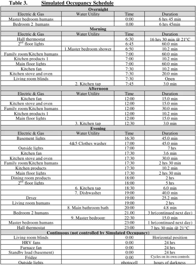
houses. A target of 20 kWh per day of electricity consumption was set, which corresponds to an accepted standard used for modelling energy systems in houses [Swinton and Sander, 1992]. As is explained below, the target was overshot by a considerable margin, and some adjustments were made. The simulated occupancy schedule is in Table 3.
ANALYSIS APPROACH
The analysis approach commonly used in side-by-side monitoring consists of comparing the energy performance of one building against the other for selected time intervals, over a selected period of time. The time interval is typically one day, as used in the BRE Test Houses in the UK [Rayment, 1998], and in Oakland for side-by-side office testing [Lee et al, 1998]. Each day is a considered to be a separate experiment in which identical sequence of events occur both within the house (using the simulated occupancy) and outdoors (weather). The results are reported on a graph of daily results, on which the consumption of one house is plotted against the other. Through varying exterior conditions, a plot is developed of these daily experimental results over time, and a statistical relation is found between the operating characteristics of each house. An example such a graph is shown in Figure 1, which is discussed later in the paper. Although the technique is deceptively simple, a number of key factors require careful consideration:
• The houses cannot simply be assumed to be identical, and calibration is essential. The assessment of innovative technologies requires a characteristic benchmark line – a performance characteristic relating the test house performance in its benchmark configuration to the reference house performance, for all cases. The technology that is assessed in the test house is therefore not compared directly to that of the reference, it is compared to the performance of what the benchmark equipment would be in the same house
under the same conditions. The distinction is important if the houses turn out not to be perfectly identical, as was the case for the hot water consumption, discussed below. The development of benchmark characteristic allows for slight differences between the houses, without affecting the accuracy of the assessment of a technology.
• The period chosen for analysis (e.g. 24 hours) and the time of day chosen for start and end of the 24 period have an influence on the scatter of the result. For example, plots prepared of the same data on a morning to morning basis had different scatter that plots produced on an afternoon to afternoon basis. Time lag in the building’s energy system, the cyclic nature of heating system operation, as well as the scheduled events during the day, all can carry the effects caused by events in one 24 hour period to show-up in the next. These effects are not necessarily synchronized between the houses. As well, meter accuracy and consumption have an effect on the scatter. A 24 hour midnight-to-midnight analysis was shown to minimize these effects. This analysis period could be revisited for assessing systems that would involve thermal mass, where lag effects might require longer periods of analysis.
• Meter resolution also needs to be considered when setting the period of analysis. For
instance, our electric meters were originally specified with a resolution of one kilowatt-hour. This was sufficient for analysis of overall house consumption, but for the analysis of daily consumption of smaller appliances such as the dishwasher (with the drying cycle turned off), the truncation error of the meter was the same order of magnitude as the consumption. As a result, the minimum period of analysis for consumption comparisons of individual
appliances was found to be at least a week. A plan for the replacement of all electrical meters with units that are accurate to the third of a watt-hour was underway at time of
writing. This will allow hourly comparisons of consumption - needed for identifying and debugging anomalies more quickly.
MONITORING AND COMMISSIONING
The first winter of operation started in January 1999 and continued until the heating season ran out in early May. During this period, the houses were finalized, debugged and commissioned. The key objective of the commissioning exercise was to ensure that all of the operating
characteristics of the houses were understood and characterized for all operating conditions. As a result, when performing experiments involving other technologies, all resulting differences between house performance could be confidently attributed to performance of the technology and not to some undocumented anomaly in facility performance. This proved to be a daunting task. The following is a discussion of the anomalies and resulting changes.
Although the high efficiency furnaces appeared to be identical, one air circulation fan motor consumed 30% less energy than the other. Not having an independent benchmark to determine which one was defective, and after prolonged debugging attempts by the contractor, both motors were replaced and rewired, eliminating the difference. It turned out that the fan motor
consuming 30% more had been correctly installed and wired in the first place – it was delivering full power, the other was not. A check of fan motor speed settings and airflow rates through the system would have probably uncovered and solved the problem more quickly. Such an
installation problem would likely go undetected by homeowners, under similar circumstances. Policing the entry of visitors and coordinating researchers in the houses was a problem.
• Initial tours of the completed houses resulted in people continually breaking visiting rules by flicking light switches and pressing control buttons. The worst such example
was a heat recovery ventilator (HRV) control setting that was changed from its original position resulting in far more high speed cycling in one house than the other. This resulted in the large scatter of data shown in Figure 1. Resetting these controls and carefully balancing and monitoring HRV performance was the single largest factor in eliminating scatter in performance between the houses.
• Monitoring the indoor air quality just after final closing of the houses was a priority. As a result, the equipment used for this process was allowed to be placed within the reference house (unlike other monitoring equipment, in the isolated control room in the garage). Unfortunately the resulting imbalance in total house heating consumption was only detected later, once the analysis technique was put in place. This effect is clearly shown by the 20.7 MJ/day offset in Figure 1. The test house required more heating due to the absence of the approximately 275 W of internal gains associated with the temporary IAQ monitoring equipment in the reference house. The
preliminary slope of the line in Figure 1 hinted at the near perfect match of the houses, confirmed in the next heating season when most of the anomalies were found and resolved.
• It can be seen in Figure 1 that as commissioning progressed into the spring of 1999, towards the lower end of the consumption curve in Figure 1, the scatter was reduced considerably.
Eventually, actual tours into the houses were stopped altogether, except under very special circumstances. Virtual tours from the neighboring information centre using computer links, were set-up to satisfy that demand.
• Temperatures at the interior surface of windows appeared to be anomalous on cold sunny days. Figure 2 shows such a profile on a day that started with a low of –20 ºC. The interior surface temperature reached above 45ºC. This was originally believed to be measurement error of the thermocouples placed on the window surface with a small bead of white cementitious compound, due to a different balance of the radiative components of heat transfer at the bead. However, independent measurements with an IR-based sensing device were within 1ºC of all thermocouple measurements. Local shading of the thermocouple bead only reduced apparent surface temperatures by 1ºC. The interior surfaces of the south facing windows were very hot to the touch. These high temperatures are apparently associated with the high performance characteristics of the window, possibly caused by a postulated high absorptance of the low-e coating on surface 3 of the sealed unit. These window properties need to be characterized in more detail. The same windows in occupied south-facing offices nearby are associated with high levels of discomfort from overheating, due to the relatively large size of these windows. This is an unresolved issue at time of writing.
• The furnace fans, once they were set to operate at the same power consumption, were
initially run continuously at high speed for better air distribution and mixing. This resulted in consumption rates of 500 W continuous, or 12 kWh per day on average, effectively blowing the targeted power budget of 20 kWh per day by a large margin – see Figure 3. These fans were subsequently reset to operate at low speed on a continuous basis, and only kick into high speed during furnace (or air conditioner) operation. This reduced furnace fan consumption to approximately 8.6 kWh/day. A higher efficiency motor in one of the technologies investigated later consumed only 7.2 kWh/day, while delivering slightly more airflow. ECM technologies would presumably do even better.
• The draw of hot water over a thermocouple in the hot water line downstream of the water heater results in the temperature profile recorded in Figure 4. The spikes were used as a standard characteristic of the simulated occupancy’s water using devices in operation, which was used to verify proper operation of each hot water using device. Typical total daily consumption of hot water was measured to be 268 L/day on average in the reference house and 279 L/day in the test house. The difference was the result of small cumulative
differences in each device, and was therefore difficult to correct, because the flow rates were determined by tap settings that could only be set in approximately the same position in each house. Appliance settings were also fixed and did not provide opportunity for fine-tuning. This difference was accepted and accounted for in the benchmarking. The differences did not bias the comparisons, just positioned the benchmark with an offset – see Figure 5.
• Not having actual occupants posed a heightened need for review of all monitored characteristics on a very regular basis during commissioning:
• solenoid operation of the shower failed to turn-it off on one occasion resulting in an 8-hour shower, with high humidity throughout the house.
• On one occasion, the stove was inadvertently left ‘on’ by the simulated occupancy for 12 hours overnight, and only turned off at its scheduled time in the morning. This event went undetected for several days. Later, comparison of daily stove consumption in both houses confirmed that the problem was with the stove in the reference house – but did not give the full picture of what had happened. Detailed review of temperature measurements in the kitchen area showed that the area over the stove had been much warmer than other areas of the house, and this data helped isolate that exact start and stop time of the event. Review of our logs revealed that a manual change of automation system clocks for
daylight saving time in spring was not properly coordinated with the simulated occupancy schedule. This resulted in the elimination of the hour in which the stove is normally turned off.
• Two thermostats were installed in each house – a regular electronic thermostat and one which is programmable through the simulated occupancy system. In the early stages, the controlled thermostat of the simulated occupancy system was used. The control system was not completely debugged at that stage. On one occasion, the simulated occupancy controller froze, and the thermostat was stuck in the ‘on’ position. The indoor
temperature reached 38ºC (100ºF) before the problem was noticed. The electronic thermostat was used until the entire simulated occupancy system was debugged. As a result of these and many other commissioning experiences, operating procedures and checklists were refined and adhered to, which resulted in a much higher level of confidence in the results.
Benchmarking
The objective of benchmarking was to account for any remaining post-commissioning
differences between the houses, and record these statistically, to give a point of reference for any future technology assessments. Benchmarking the houses occurred over the period from
November 1999 to the end of January 2000. Figure 5 shows the results for hot water heating, with slight scatter and an offset. The test house consumed about 18% more energy for hot water heating than the reference house. The higher consumption of the test house is related to a number of cumulative factors that are difficult to control. Slightly greater hot water draws were noted in the test house as discussed above, and there was poor control over actual water heater
for fine-tuning. Nevertheless, this offset became part of the benchmarked condition, and therefore would not affect future comparisons, which will take this offset into account. It was also important to remember that the documented difference in hot water consumption also plays a role the in the space heating system which was benchmarked concurrently. Refining the hot water situation would necessitate re-benchmarking the space heating as well, which undesirable to do, given time and resource constraints and the satisfactory result described below.
Benchmarking the space heating consumption, theoretically the more challenging exercise, turned out to be simpler in that the results confirmed that the objective of the design was met – virtually overall identical thermal performance, on a statistical basis. Figure 6 shows the benchmarking of the test house against the reference over the same period. It is noted that whereas each day’s result is not necessarily a perfect match, statistically, this is a near-perfect result, with the slope being measured only 0.7% lower than a perfect fit with a slope of “1”. We interpret this result as follows, small differences associated with daily comparisons appear to be random, and cancel out, given a large enough sample of points. As well, the house airtightness and hot water consumption were both documented to be slightly different, so it is important to note that the excellent space heating correlation is the results of the net cancellation of many small differences in the house’s total energy system.
Experience in interpreting results of subsequent assessments with this facility suggests that approximately two to three weeks of data (14 -21 data points) are sufficient to give a good statistical estimate of performance, provided that the weather patterns in that period are
shown in these figures. A strategy of alternating technologies from week to week was adopted to ensure that each technology was operated in different conditions throughout the heating season.
Finally, the benchmark line needed for assessing heating systems that supply both space heating and hot water is calculated by finding the total of the benchmark result for hot water heating and that for space heating, resulting in the characteristic shown in Figure 7. That benchmark of total gas consumption was checked later in the heating season, after several weeks of experiments and it essentially remained intact, as shown by the data points which mostly touch the previously derived benchmark line.
Figure 8 illustrates how the facility and analysis procedures are used to assess the performance of two technologies against the benchmark. On days where data points for a given technology fall above the benchmark line, that technology consumes more than the benchmark configuration, and vice versa. The fact that the characteristic performance lines of the technologies cross the benchmark line turned out to be due more to the moving target offered by the benchmark than due to changes in performance of the technology. The explanation is as follows: the benchmark for space heating is based on high efficiency condensing technology (e.g. 91%). The benchmark for water heating is based on conventional technology (e.g. 67%), as specified in Table 1. At any given point during the heating season, the overall combined efficiency of the benchmark heating equipment is a combination of the two efficiencies, in proportion to the relative size of space heating load to hot water heating load. Once this was realized, it became clear that the technologies used for space and water heating should be as close as possible in efficiency, to present a relatively fixed efficiency target for combined heating equipment technologies.
The strong statistical linear fit of these performance lines suggests that the characteristic could be used to assess over all seasonal performance comparisons, based on approximately three weeks of testing for each technology.
CONCLUSIONS
In 1998, twin houses were built at the Canadian Centre for Housing Technology in Ottawa to assess the energy performance of new and innovative energy efficient materials and components for houses. This paper describes the energy features of the houses, commissioning and
benchmarking results. With the benefit of detailed monitoring of energy systems in both houses, many of the anomalies in component operation and controls were rectified. Close monitoring and supervision of the operation of the houses was shown to be a necessary element of gaining full control over their operation. Once commissioned, the houses were shown to perform in a near-identical fashion. Remaining differences were benchmarked in a detailed fashion, to ensure that the performance characteristics attributed to new technologies by this facility would be solely attributable to the technology and not to unaccounted anomalies in the operation of the facility. The resulting facility was shown to be capable of delineating performance differences with a high level of accuracy. A two to three week monitoring period for each technology was found to be sufficient for performance comparison purposes.
ACKNOWLEDGEMENTS
The authors wish to thank Frank Szadkowski, Dr. Evgueniy Entchev of Natural Resources Canada for assisting in the commissioning of HVAC equipment and their performance characterization in the houses. The authors would also like to thank Ludo Bertsch and Neil Morris of Horizon Technologies for assisting with the design and specification of the simulated occupancy system and who assisted with commissioning and debugging the system. Finally, special thanks to Luc Saint-Martin, Business Manager of CCHT and Dr. Nady Said for their review of the paper.
REFERENCES
Brown, W.C., 1980. Mark XI Energy Research Project - Comparison of Standard and
Upgraded Houses. Division of Building Research (now Institute for Research in Construction), National Research Council Canada. Building Research Note No. 160, June 1980.
Lee, E.S. DiBartolomeo, D.L. and Selkowitz, S.E. 1998. Thermal and Daylighting
Performance of an automated venetian blind and lighting system in a full scale private office. Energy and Buildings 29, 1998, 47-63.
Quirouette, R.L., 1978. The Mark XI Energy Research Project – Design and Construction. Division of Building Research (now Institute for Research in Construction), National Research Council Canada. Building Research Note No. 131, October 1978.
Rayment, R., Hart, J., and Whiteside, D. 1993. The DoE/BRE Energy and Environment Test Houses. Building Research Establishment Internal Report N196/92, January 1993.
Rayment, R., Hart, J., and Whiteside, D. 1997. Comparison of moisture clearance by trickle and ducted systems in Swedish test houses. Building Research Establishment Internal Report N101/97, August 1997.
Swinton, M.C. and Sander, D.M. 1992 "Economic levels of thermal resistance for house envelopes: considerations for a national energy code". Renewable Energy -- Technology for Today : Conference Proceedings : 18th Annual Conference for the Solar Energy Society of Canada (Edmonton, ALBT, Canada, 1992) pp. 165-170, 1992. (NRCC-34019) (IRC-P-1804)
Table 1. Selected Characteristics of the Houses Component Characteristic
Construction Standard R-2000
Storeys 2
Liveable Area 210 m2
Basement Poured concrete, full basement.
Garage Two-car, recessed into the floor plan; isolated control room in the garage
Attic RSI 8.6
Walls RSI 3.5
Rim Joists RSI 3.5
Exposed floor over the garage
RSI 4.4 with heated/cooled plenum air space between insulation and sub-floor.
Basement Walls RSI 3.5 in a framed wall. No vapour barrier. Basement floor Concrete slab, no insulation
Windows Low-e, insulated spacer, argon filled, with argon concentration measured to 95%.
Window Area South Facing: 16.2 m2 Total: 35.0 m2
Air Barrier System Exterior, taped fiberboard sheathing with laminated weather resistant barrier. Taped penetrations, including windows.
Airtightness Reference 1.07 ach @ 50 Pa; Test House 0.97 ach @ 50 Pa Heat recovery Ventilator High Efficiency (84% nominal)
Furnace Condensing gas @ 91% efficiency (as measured)
Hot Water Heater Conventional, induced draft @ 67% efficiency (as measured). Air conditioning High efficiency - SEER 12 (nominal)
Table 2. List of meters installed in Each House.
Electric Meters Gas Meters
1 Heat Recovery Ventilator 1 Furnace
2 Furnace 2 Hot Water Heater
3 Dishwasher
4 Clothes Washer Water Meters
5 Refrigerator 1 Main (entire house) 6 Air Conditioner 2 Second Floor
7 Dryer 3 DHW
8 Stove 4 Kitchen Sink
9 Main Panel 5 Dishwasher
10 Lights & Receptacles 11 Control Room 12 Exterior Lights
13 Brown Plates (Monitoring) 14 DHW power vent Fan
Table 3. Simulated Occupancy Schedule Overnight
Electric & Gas Water Utility Time Duration
Master bedroom humans 0:00 6 hrs 45 min
Bedroom 2 humans 0.00 6 hrs 45min
Morning
Electric & Gas Water Utility Time Duration
Hall thermostat 6:30 16 hrs 30 min @ 21°C
2nd floor lights 6:45 60.0 min
1.Master bedroom shower 6:50 10.2 min
Family room/Kitchen humans 7:00 60.0 min
Kitchen products 1 7:00 10.2 min
Main floor lights 7:00 60.0 min
Kitchen fan 7:30 10.2 min
Kitchen stove and oven 7:30 20.0 min
Living room blinds 7:30 Open
2. Kitchen tap 7:45 3.0 min
Afternoon
Electric & Gas Water Utility Time Duration
Kitchen fan 12:00 15.0 min
Kitchen stove and oven 12:00 15.0 min
Family room/Kitchen humans 12:00 30.0 min
Kitchen products 1 12:00 10.2 min
Main floor lights 12:00 15.0 min
3. Kitchen tap 12:30 3.0 min
Evening
Electric & Gas Water Utility Time Duration
Basement lights 16:30 45.0 min
4&5 Clothes washer 17:00 45.0 min
Outside lights 17:00 7 hrs
Kitchen fan 17:30 3.6 min
Kitchen stove and oven 17:30 30.0 min
Family room/Kitchen humans 17:30 2 hrs 30 min
Kitchen products 17:30 10.2 min
Main floor lights 17:30 2 hrs 30 min
Dining room products 18:00 2 hrs
2nd floor lights 18:00 5 hrs
6. Kitchen tap 18:30 6.0 min 7. Dishwasher 19:00 40.0 min
Dryer 19:00 25.2 min
Living room humans 19:00 2 hrs
8. Main bathroom bath 20:00 4.8 min
Bedroom 2 humans 21.00 3 hr(continued next day) 9. Master bedroom 22:30 15.0 min Master bedroom humans 23:00 1 hr(continued next day)
Hall thermostat 23:00 7 hrs 30 min @ 21°C
Continuous (not controlled by Simulated Occupancy)
Living room blinds 0:00 Horizontal position
HRV fans 0:00 24 hrs
Furnace fan 0:00 24 hrs
Standby load (basement) 0:00 24 hrs
Fridge 0:00 Cycles on its own controls
FIGURE CAPTIONS
Figure 1 Pre-commissioning benchmark data for space heating and statistically fitted line. Figure 2. Sunny day profile of interior and exterior glazing surface temperatures
Figure 3. Comparison of average daily electricity consumption of both houses measured over one week. (The heat release from people, simulated with lamps, is recorded
separately, but added here to show total internal heat gain).
Figure 4. A thermocouple placed in the hot water line downstream of the water heater records pipe water temperature rise and drop, as water using devices are turned on and off
Figure 5. Benchmark data for domestic water heating. (Shown on a scale consistent with the space heating graphs for comparison).
Figure 6 Post-commissioning benchmark data for space heating and statistically fitted line.
Figure 7 Verification of benchmark of total gas consumption (space and water heating combined) during assessment of technologies.
Figure 8 Example assessment of two technologies using the benchmark for total gas consumption as a reference.
Comparison of Heat Consumption for Space Heating of the CCHT Houses
0 100 200 300 400 500 600 0 100 200 300 400 500 600
Heat Consumption - Reference House, MJ/day
Heat Consumption -Test House, MJ/day
Slope = Intercept = Correlation Coefficient = 1.002 20.7 0.965 Jan 6 - May 12, 1999 Benchmark Characteristics - Pre-commissioning Line of perfect agreement (Slope =1)
Fitted line: pre-commissioning benchmark
Pre-Commissioning
CCHT Reference House - South Facing Window Temperatures (February 17, 2000, -20C and sunny)
-15 -5 5 15 25 35 45 55 0:00:00 17-Feb-00 3:00:00 17-Feb-00 6:00:00 17-Feb-00 9:00:00 17-Feb-00 14:00:00 17-Feb-00 17:00:00 17-Feb-00 20:00:00 17-Feb-00 23:00:00 17-Feb-00
Date & Time
Temperature,
0 C
Outer Pane Inner Pane
47.53 C 12.77 C 32°F 5°F 77°F 113°F
Total Electrical Consumption - CCHT Research Houses 0 5 10 15 20 25 30
Ref Dec 4-10 Test Dec 4-10
Date
Daily Average Electricity Consumption, kWh/day
Furnace HRV Int.lights & plugs Stove Fridge Dish/r Washer Dryer Simulated People People energy separated
from total electricity consumption
Daily Profile of Water Temperature in Pipe Downstream of Water Heater 30 35 40 45 50 55 60 65 70 0 6 12 18 24 Time, hours Temperature, °C Shower Kitchen Tap Kitchen Tap Clothes Washer Fill & Rinse
Kitchen Tap Dishwasher Bath Shower 104°F 122°F 140°F 158°F
Benchmark of Gas Comsumption for Hot Water Heating 0 100 200 300 400 500 600 0 100 200 300 400 500 600
Reference House Consumption, MJ/day
Test House Consumption, MJ/day
Note: 100 MJ ~ 95 kBTU
Line of perfect agreement (Slope =1)
Consumption for Space Heating in CCHT Research Houses
0 100 200 300 400 500 600 0 100 200 300 400 500 600Reference House Consumption, MJ/day
Test House Consumption, MJ/day
Benchmark Data Perfect Fit Fitted Line
Slope = Intercept = Correlation Coefficient = 0.993 1.371 0.997 Benchmark Characteristics
Benchmark Data - Nov 12, 1999 to Jan 24, 2000
Post-Commissioning
Verification of the Benchmark - Combined Space and Water Heating 0 100 200 300 400 500 600 0 100 200 300 400 500 600
Reference House Consumption, MJ/day
Test House Concumption, MJ/day
Original Benchmark - Fitted Line Verification Data Points
Original Benchmark Characteristics
Slope= Intercept =
0.993 17.0 Verification data measured the weeks of March 6 and May 13, 2000
Two Technologies Assessed
0 100 200 300 400 500 600 0 100 200 300 400 500 600Reference House Consumption, MJ/day
Test House Consumption, MJ/day
Benchmark Technology 1 Fitted Tech.1 Technology 2 Fitted Tech. 2
Benchmark
Technology 2 System Characteristics
Slope = Intercept = Correlation Coefficient = 1.149 -26.7 0.998
Technology 1 System Characteristics
Slope = Intercept = Correlation Coefficient = 1.238 -14.3 0.998 February 2 to April 2, 2000 Note: 100 MJ ~ 95 kBTU