HAL Id: hal-03040390
https://hal.archives-ouvertes.fr/hal-03040390v2
Preprint submitted on 23 Dec 2020
HAL is a multi-disciplinary open access archive for the deposit and dissemination of sci-entific research documents, whether they are pub-lished or not. The documents may come from teaching and research institutions in France or abroad, or from public or private research centers.
L’archive ouverte pluridisciplinaire HAL, est destinée au dépôt et à la diffusion de documents scientifiques de niveau recherche, publiés ou non, émanant des établissements d’enseignement et de recherche français ou étrangers, des laboratoires publics ou privés.
Construction of parsimonious event risk scores by an
ensemble method. An illustration for short-term
predictions in chronic heart failure patients from the
GISSI-HF trial.
Benoît Lalloué, Jean-Marie Monnez, Donata Lucci, Eliane Albuisson
To cite this version:
Benoît Lalloué, Jean-Marie Monnez, Donata Lucci, Eliane Albuisson. Construction of parsimonious event risk scores by an ensemble method. An illustration for short-term predictions in chronic heart failure patients from the GISSI-HF trial.. 2020. �hal-03040390v2�
1 Full title: “Construction of parsimonious event risk scores by an ensemble method. An illustration for short-term predictions in chronic heart failure patients from the GISSI-HF trial.”
Short title: “Construction and illustration of parsimonious event risk scores by an ensemble method.”
Benoît Lalloué1,2,*, Jean-Marie Monnez1,2, Donata Lucci3, Eliane Albuisson4,5 6
1
Université de Lorraine, CNRS, Inria (Project-Team BIGS), IECL (Institut Elie Cartan de Lorraine), Nancy, France;
2
Inserm U1116, Centre d'Investigation Clinique Plurithématique 1433, Université de Lorraine, Nancy, France;
3
ANMCO Research Center, Florence, Italy;
4
Université de Lorraine, CNRS, IECL (Institut Elie Cartan de Lorraine), Nancy, France;
5 BIOBCHRU-Nancy, DRCI, Nancy, France; 6
Faculté de Médecine, InSciDenS, Vandœuvre-lès-Nancy, France.
E-mail: benoit.lalloue@univ-lorraine.fr (BL); jean-marie.monnez@univ-lorraine.fr (JMM); donata.lucci@anmco.it (DL); eliane.albuisson@univ-lorraine.fr (EA)
2
Abstract
Heart failure (HF) is a worldwide major cause of mortality and morbidity for which many predictive scores have been defined. Selecting which explanatory variables to include in a given score is a common difficulty, as a balance must be found between statistical fit and practical application. This article presents a methodology for constructing parsimonious event scores combining a stepwise selection of variables with ensemble scores obtained by aggregation of several scores, using several classifiers, bootstrap samples and various modalities of random selection of variables. The stepwise selection allows constructing a succession of scores, with the practitioner able to choose which score best fits his needs. The methods proposed herein can be reproduced on any set of variables as long as the training dataset comprises a sufficient number of cases.
Three methods were compared in an application to construct parsimonious short-term scores in chronic HF patients, two involving a backward selection of the variables based on their coefficients in an ensemble score and the third involving a forward selection of the variables maximizing the AUC. The working sample consisted of 11,411 (patient, visit) couples from the GISSI-HF database, with 5,595 events (duplicated in order to balance the sample) and 5,816 non-events. Sixty-two candidate explanatory variables were studied. The outcome was the composite endpoint of death or hospitalization for worsening HF within 180 days of a visit. The three methods yielded a selection of 50, 59 and 26 variables, respectively. For a given number of selected variables, most were common to the three methods. Focusing on the fastest method, four scores were constructed, yielding out-of-bag AUCs ranging from 0.81 (26 variables) to 0.76 (2 variables). These results are slightly better than those obtained by other scores reported in the literature using a similar number of variables.
1. Introduction
Heart failure (HF) is a global and major cause of mortality and morbidity. This disease carries a burden both on the patients themselves, who suffer from a lower quality of life and reduced life
3 expectancy, as well as for the healthcare systems, particularly due to hospitalization costs [1,2]. Successfully predicting the course of the disease could therefore help alleviate this burden.
The association between HF outcomes (death, hospitalization, device implantation, transplantation, etc.) and a large number of variables (whether demographic, clinical, biochemical, biomarkers, etc.) has been widely highlighted in the literature. A common approach to usefully synthesize the information provided by this large number of predictor variables is to create a risk score aimed at predicting the probability of adverse events. Many predicting scores and models have already been published: in a recent literature review, Di Tanna et al. [3] identified 58 risk-prediction models for HF in 40 articles published between 2013 and 2018. A much larger number of these models have furthermore been published over the last three decades [4–7].
Scores are mainly constructed using “classic” statistical methods. Among the 40 recent articles studied, Di Tanna et al. [3] counted 11 studies using logistic regressions (mostly binary and multivariate) and 22 using Cox regressions (mostly multivariate and stepwise). Scores using other methods, such as machine learning methods, are rarer although increasingly proposed nowadays [8– 10]. In the study of Duarte et al. [11], the authors proposed a methodology for constructing a short-term event risk score in HF patients based on the use of an ensemble method involving two classification rules (logistic regression and linear discriminant analysis), bootstrap samples as well as introducing random selections of variables in the construction of predictors. The principle of an ensemble method is to build a collection of predictors and thereafter aggregate the predictions [12], a well-known example being the random forests method [13]. An ensemble predictor is expected to be better than each of the individual predictors, provided that (i) each single predictor is relatively good and (ii) single predictors are sufficiently different from each other [14]. Other studies have used various forms of ensemble methods without designating the latter as such, for example by constructing multiple imputed datasets, drawing bootstrap samples on each of these datasets, and subsequently building models on each sample prior to their aggregation [15–17].
4 A common difficulty in the construction of prognostic scores is to choose which variables to include in the model. Indeed, the more variables are contained in a model, the more complicated its use in clinical practice. Therefore, a balance must be found between increasing the number of variables to allow for a better statistical fit and keeping this number sufficiently small to facilitate practical application. With the increased number of potential predictors (through the use of "big data" from both electronic medical records and the increasing number of available biomarkers), the need for the statistical selection of variables also increases, particularly if the goal is to continue building parsimonious and effective models. Variables can be selected using a literature review in order to assess which variables are the most clinically relevant [18,19]. This often constitutes a preliminary step before using various methods of statistical selection. Among the statistical methods, a simple method is to retain only the significant variables derived from univariate analyses [20–22] or from a full multivariate model [23,24]. Slightly more elaborate methods such as stepwise selection can also be used [15,25]. Finally, certain studies select variables with more complex methods, using bootstrapping [17], random forests and decision trees [10,26] or other selection methods [27]. Since the primary goal in the present study is to construct a score using an already-defined ensemble method, most of the above selection methods are not easily applicable in this setting. For example, the likelihood ratio test based on a probabilistic model can be used to achieve a stepwise selection for a given classifier such as logistic regression but not directly for an ensemble method. Other selection criteria must hence be defined.
Given this context, this article presents a methodology for constructing parsimonious event scores combining a stepwise preselection of variables and the use of ensemble scores. In particular, we define herein three methods, two of which involve a backward selection based on the variables’ coefficients in an ensemble score, and the third involving the combination of a forward selection using the area under the ROC curve (AUC) as criterion and an ensemble score. Due to the stepwise selection, a succession of scores is constructed which allows the user to choose which of the latter yield the best balance between performance and the number of variables. As a concrete illustration,
5 these three methods of construction of parsimonious scores are compared according to AUC and processing time in an application aimed at constructing short-term scores in chronic heart failure (CHF) patients.
2. Methods
2.1.
First exclusion of variables
Univariate tests (Wilcoxon test for continuous variables and Fisher’s exact test for categorical variables) were first used to test the association between the response variable and each explanatory variable. Variables with a p-value greater than 0.2 were excluded.
2.2.
Construction of an ensemble score
The methodology detailed in Duarte et al. [11] was adapted to construct the scores. Basically, it used an ensemble method, where several models were built using various classification methods, different samples and different variable selections, and were subsequently aggregated in a unique score by averaging. This method can be described in seven phases (with specific choices summarized in Figure 1), as follows:
1. n1 classifiers are chosen. Two classifiers, linear discriminant analysis (LDA), which is
equivalent to linear regression on binary outcomes, and logistic regression (LR) were chosen. 2. n2 bootstrap samples are drawn from the working sample. Each bootstrap sample is used n1
times (each sample is used by each classifier). In the present instance, n2 = 1000.
3. n3 modalities of selection of variables are chosen, “modality” representing a means to select
the variables. In the present instance, n3 = 2: namely, one modality to randomly draw a
defined number of variables, the other to randomly draw a defined number of groups of related variables (correlated or linked by construction) and, for each selected group, randomly draw one variable. The groups of related variables used in the application are shown Table 1.
6 4. n1n2n3 models are built, each using a different combination of classifiers, bootstrap samples
and modalities of selection of variables.
5. A first aggregation by classifiers is performed. The coefficients of the models are averaged to yield n1 intermediate scores. In the present instance, one score was constructed for linear
discriminant analysis (SLDA) and the other for logistic regression SLR.
6. The coefficients of the intermediate scores are normalized such that the scores themselves are between 0 and 100, using the same method as in Duarte et al. ([11], Subsection 4.4.2). The two normalized scores were denoted and .
7. The final score is constructed by taking an affine combination of the intermediate scores. In the present instance, ( ); the optimal value of λ was
determined by testing values from 0 to 1 using incremental 0.01 steps and selecting the value maximizing the out-of-bag AUC (see below).
Figure 1. Methodology of construction of the ensemble score
Compared to the methodology presented in Duarte et al. [11], a balanced sample was used, and the normalization of the coefficients was carried out before rather than after the final aggregation. The latter change was made to balance the intermediate scores in the event that their raw coefficients would have different orders of magnitude.
2.3.
Preselection of variables and construction of
parsimonious scores
As the number of explanatory variables after the first exclusion of variables still remained too large to create a parsimonious score, a second phase was added in order to preselect a fewer number of variables. Three different methods with an additional preselection were proposed and their results compared.
7
Preselection of variables: For LDA and for LR, a stepwise preselection using the Akaike Information
Criterion (AIC) was performed on the working sample, without bootstrapping. Thus, two sets of preselected variables were created. The union of these two sets was used as initial preselection. Let be the number of preselected variables.
Note that herein, the AIC can be used as criterion since both LDA and LR are probabilistic models. With non-probabilistic classification rules, AIC could not be used. However, in general, any preselection method could be used in this phase.
Construction of scores: For i = 1, 2, …, s: at step i: an ensemble score was constructed from j = s – i + 1
variables (i.e., for i = 1, j = s ; for i = s, j = 1), using two classifiers (LDA and LR), 1000 bootstrap samples, two modalities of selection of variables (all variables or all groups of related variables). The variable with the lowest normalized and standardized coefficient in absolute value in this score was excluded for the step i + 1 (backward selection).
This allowed determining the evolution of the AUC OOB according to the number of selected variables, as well as the order of removal of the variables. Parsimonious scores with few variables can be chosen among this sequence of s scores.
2.3.2. Method 2
Preselection of variables: No initial preselection of variables was performed; all of the 64 explanatory
variables were included.
Construction of scores: For i = 1, 2, …, 64: at step i: an ensemble score was constructed from j = 64 – i
+ 1 variables (i.e., for i = 1, j = 64 ; for i = 64, j = 1), using two classifiers (LDA and LR), 1000 bootstrap samples and two modalities of selection of variables (a random selection of 75% of the variables or of 75% of the groups of related variables). The variable with the lowest normalized and standardized coefficient in absolute value in this score was excluded for the step i + 1.
8 Again, this process allowed determining the evolution of the AUC OOB according to the number of selected variables, as well as the order of removal of the variables, and parsimonious scores with few variables can be chosen among this sequence of 64 scores.
2.3.3. Method 3
Preselection of variables: A forward preselection using AUC as criterion was performed using LR. Let t
denote a stopping time. For i = 1, 2, …, t, at step i: i – 1 variables denoted V1, …, Vi-1 were available
from step i - 1; for every set of variables V1, …, Vi-1,Vj with j ≠ 1, …, i - 1, a logistic regression was
performed on the entire sample without bootstrap; the variable, denoted Vi, yielding the maximal
AUC in resubstitution was included for the step i + 1, provided that the AUC significantly increased using DeLong’s test; otherwise, the inclusion of variables was stopped (t = i).
Note that, contrary to the preselection phase of Method 1 with AIC, there is no need in this instance for a probabilistic model. Indeed, the AUC can be computed as long as there is a prediction for each statistical unit, without assumption on the manner with which this prediction was obtained.
Construction of intermediate scores: For each classifier, intermediate scores using only the
preselected variables, with the transformations corresponding to the classifier (see Subsection 3.2.4), were constructed, using 1000 bootstrap samples (the same for both classifiers) and two modalities of selection of variables (all variables or all groups of related variables).
Construction of final scores: The two intermediate scores using the same number of preselected
variables were aggregated in a final score by averaging their prediction for each statistical unit. Other methods were tested although not shown here. Their descriptions and results are available as Supplementary Material (Part A).
2.4.
Comparison criteria between the methods
The area under the ROC curve (AUC) for the out-of-bag (OOB) estimations was used as internal validation and as the main criterion to compare the different scores. The OOB AUC was computed as
9 follows: for a given statistical unit, the scores obtained from bootstrap samples that did not include this statistical unit were aggregated to obtain an OOB prediction. By applying this method for all statistical units, OOB predictions for the entire sample were used to compute the AUC OOB. Three AUC OOB were studied: the AUC OOB for the intermediate linear score, the AUC OOB for the intermediate logistic score and, mainly, the AUC OOB for the global score.
Sensitivity (Se) and specificity (Sp) corresponding to the highest Youden index (Se + Sp - 1), as well as the number of selected variables and processing time, were also taken into account.
3. Application for short-term predictions in chronic heart
failure patients
3.1.
Description of the original data
The data used in this study are derived from the GISSI-HF trial: a multicenter, randomized, double-blind, placebo-controlled trial designed to assess the effect of n-3 polyunsaturated fatty acids in patients with CHF. The detailed protocol and main results of this trial have already been described elsewhere [28,29].
Eligible patients were adult men and women with clinical evidence of HF of any cause, with a New York Heart Association (NYHA) class II–IV, and having had a left ventricular ejection fraction (LVEF) measured within 3 months prior to enrolment. Patients with a LVEF greater than 40% had to have been admitted at least once to hospital for HF in the preceding year to meet the inclusion criteria. In addition to contraindications linked to the studied treatment, exclusion criteria included acute coronary syndrome or revascularization procedure within the preceding 1 month; and planned cardiac surgery expected to be performed within 3 months after randomization.
After randomization and the baseline visit, patients underwent scheduled visits at 1, 3, 6, 12 months and every 6 months thereafter until the end of the trial. Data collected at baseline included patient
10 description, medical history, etiology of HF, LVEF measurements, electrocardiogram data, clinical and cardiovascular examination, blood chemistry tests, pharmacological treatments and dietary habits. During the follow-up visits, collected data consisted of patient description, clinical and cardiovascular examination, LVEF measurement, electrocardiogram data, blood chemistry tests (only at 1, 3, 6, 12, 24, 36 and 48 months), pharmacological treatment (including the study treatment) and dietary habits. Events of interest were also recorded. The entire GISSI-HF trial included 7046 eligible and randomized patients, with the final sample analyzed in [29] and comprised of 6975 patients.
The present study used a subsample of the GISSI-HF data containing 1231 patients with N-terminal prohormone brain natriuretic peptide (NT-proBNP) measurements. The dataset included baseline and follow-up visits for these patients, as well as their associated health events.
3.2.
Data management
3.2.1. Statistical unit: (patient, visit) couples
(Patient, visit) couples were used herein as statistical units, i.e. each observation was associated to a patient for a given visit. We assumed that the short-term future of a patient was only dependent on the most recent measurements. Thus, the links between several couples pertaining to the same patient were not taken into account, as in [11,30]. This yielded an initial sample of 12,882 (patient, visit) couples.
3.2.2. Variable pre-processing
Several variables were derived from the available data, either for the follow-up visits (when values were available at baseline but not for the follow-up) or for all visits: mean blood pressure (BP) (1/3*systolic BP + 2/3*diastolic BP); estimated plasma volume (ePVS) ((100-hematocrit)/hemoglobin as defined in [31]); estimated glomerular filtration rate (eGFR) (using the MDRD formula [32]); age and body mass index (BMI). Binary variables for the therapeutic classes of drugs were also derived
11 from detailed information pertaining to pharmacological treatments in order to indicate the consumption of ACE-inhibitors, beta-blockers, calcium antagonists or diuretics.
Categorical variables were recoded as binary dummy variables. In particular, in the case of ordinal variables (i.e. NYHA class and peripheral edema), an ordinal encoding was used, namely constructing the binary variables NYHA ≥ II, NYHA ≥ III and NYHA ≥ IV and, similarly, peripheral edema ≥ ankles, peripheral edema ≥ knee, peripheral edema ≥ above.
Since some variables were only available at baseline but were unlikely to change over time (e.g. sex), their values were copied for follow-up visits. Similarly, certain medical history variables available at baseline (such as previous acute myocardial infarction (AMI), previous stroke, angina pectoris,
coronary artery bypass graft (CABG), previous hospitalization for worsening HF) were copied for follow-up visits and, when possible, updated using the information from the events.
NT-proBNP values were only measured at baseline and at the 3-months follow-up. Due to the importance of this variable in the literature [27,33–35], it was decided to retain and interpolate its value for the other visits as follows: the value for the 1-month follow-up visit was computed as 2/3*(baseline value) + 1/3*(3-months value). Value of the 3-months visit was copied for the subsequent visits.
Lastly, the response variable was defined as the occurrence of a composite event (death for worsening HF or hospitalization for worsening HF) within 180 days of a visit.
3.2.3. Exclusion of variables and observations
Since the laboratory tests for measuring blood parameters were performed only at baseline, 1, 3, 6, 12, 24, 36 and 48 months, only the observations corresponding to these visits were retained. Incomplete observations (with missing values) were also excluded.
Several variables not relevant to this study were excluded (e.g. “technical variables”, such as identification numbers or dates, or “intermediary variables” used to build other variables, such as the
12 cause of death or drug doses), as well as variables with more than 1,000 missing values. The remaining variables are shown Table 1.
3.2.4. Transformation of the variables
In order to eliminate outliers without excluding the associated observations, all continuous variables were winsorized: all values lower than the 1st percentile (respectively greater than the 99th percentile) were set to the value of the 1st percentile (resp. the 99th percentile). This method was used to avoid excluding more observations, since the number of cases was already small compared to the controls and to avoid reducing the number of patients with event.
Continuous variables were then transformed to satisfy the linearity assumption of logistic regression. For each continuous variable, a similar method to that described in Duarte et al. [11] was used. First, the restricted cubic splines method with 3 knots was used to test the linearity assumption for each variable under the univariate logistic model: using a likelihood ratio test, the nullity of the coefficient associated with the cubic component of the spline was tested [17,27]. Then, for each variable with a significantly non-null coefficient with a 5% threshold, a graphical representation of the links between the variable and the logit was performed. If the relationship was monotonous, simple monotonic transformations of the form f(x) = xa with or f(x) = ln(x) were tested. If the relationship was not monotonous, quadratic transformations of the form f(x) = (x – k)² were tested, with k situated between the minimum and the maximum of the variable by incremental 0.1 steps. To determine the values of a or k, all possible values were tested and the transformation which yielded a non-significant p-value for the linearity test and a minimal p-value for the test of nullity of the coefficient in univariate logistic regression was retained.
This transformed dataset was used for Methods 1, 2 and the LR intermediate score of Method 3. A similar technique was used for the LDA intermediate score of Method 3, but with transformation of the variables in order to satisfy the linearity assumption for linear regression.
13
3.2.5. Sample balancing
Given the large imbalance between cases and controls, the sample was balanced by duplicating each case 15 times. This is equivalent to giving each case fifteen times more weight than a control. Preliminary analyses (not shown) showed that using a sample that was rebalanced in this manner resulted in better performance compared to using the unbalanced sample.
4. Results
Summary statistics of the sample prior to data management (winsorization, transformation of the variables and sample balancing) are available in the Supplementary Material (Part B). Summary statistics of the sample after winsorization and sample balancing, but before the transformation of the variables, are provided in Table 1.
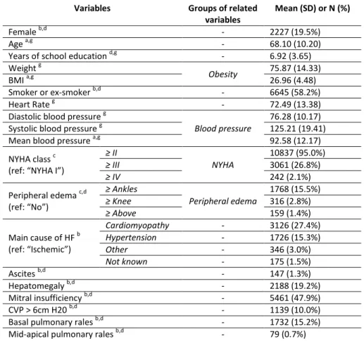
Table 1. Descriptive statistics of the explanatory variables after winsorization and sample balancing performed before transformation of the variables
Variables Groups of related
variables
Mean (SD) or N (%)
Female b,d - 2227 (19.5%)
Age a,g - 68.10 (10.20)
Years of school education d,g - 6.92 (3.65)
Weight g
Obesity 75.87 (14.33)
BMI a,g 26.96 (4.48)
Smoker or ex-smoker b,d - 6645 (58.2%)
Heart Rate g - 72.49 (13.38)
Diastolic blood pressure g
Blood pressure
76.28 (10.17)
Systolic blood pressure g 125.21 (19.41)
Mean blood pressure a,g 92.58 (12.17)
NYHA class c (ref: “NYHA I”)
≥ II NYHA 10837 (95.0%) ≥ III 3061 (26.8%) ≥ IV 242 (2.1%) Peripheral edema c,d (ref: “No”) ≥ Ankles Peripheral edema 1768 (15.5%) ≥ Knee 316 (2.8%) ≥ Above 159 (1.4%) Main cause of HF b (ref: “Ischemic”) Cardiomyopathy - 3126 (27.4%) Hypertension - 1726 (15.3%) Other - 346 (3.0%) Not known - 175 (1.5%) Ascites b,d - 147 (1.3%) Hepatomegaly b,d - 2188 (19.2%) Mitral insufficiency b,d - 5461 (47.9%) CVP > 6cm H20 b,d - 1139 (10.0%)
Basal pulmonary rales b,d - 1732 (15.2%)
14
Pulmonary rales b,d - 599 (5.2%)
Aortic stenosis b,d - 315 (2.8%)
Third heart sound (S3) b,d - 2177 (19.1%)
Hematocrit g Hematology 40.16 (4.53) Hemoglobin g 13.40 (1.60) ePVS a,g 4.57 (0.92) Serum creatinine g Renal function 1.27 (0.44) eGFR a,g,h 64.08 (22.63) Serum potassium g - 4.48 (0.50) Serum sodium g - 139.49 (3.33) Uricemia g - 6.43 (1.94) Triglycerides g - 137.92 (84.01) Cholesterol HDL g Cholesterol 47.58 (13.19) Total Cholesterol g 175.10 (44.48) Bilirubin g - 0.84 (0.42) Glycemia g - 122.98 (46.60) NT-proBNP f,g - 1856.60 (2194.91) Diabetes mellitus b,d - 3481 (30.5%) Hypertension b,d - 6470 (56.7%)
Previous AMI b,e - 5421 (47.5%)
Previous stroke b,e - 643 (5.6%)
Previous hosp. for worsening HF b,e - 6526 (57.2%)
Angina pectoris b,e - 2060 (18.1%)
Coronary angioplasty b,d - 1478 (13.0%)
Transient ischemic attack (TIA) b,d - 1228 (10.8%)
COPD b,d - 2348 (20.6%)
CABG b,e - 2847 (24.9%)
Implantable defibrillator b,d - 1020 (8.9%)
Paroxystic AF b,d - 2756 (24.2%)
Neoplasia b,d - 592 (5.2%)
Definitive pace maker b,d - 1944 (17.0%)
Waiting for cardiac transplantation b,d - 122 (1.1%)
LVEF d,g - 32.58 (10.05)
Bundle branch block b - 3883 (34.0%)
Atrial fibrillation b - 2087 (18.3%)
Left ventricular hypertrophy b - 1885 (16.5%)
Pathological Q waves b - 2236 (19.6%)
Normal ECG evaluation b - 415 (3.6%)
ACE-inhibitors a,b - 8782 (77.0%)
Beta-blockers a,b - 7430 (65.1%)
Calcium antagonists a,b - 803 (7.0%)
Diuretics a,b - 10813 (94.8%)
a
derived variable; b binary variable encoding; c ordinal encoding; d baseline value copied to follow-up visits; e baseline value copied to follow-up visits and updated when possible;
f
interpolated values; g winsorized variable
SD: standard deviation; BMI: body mass index; NYHA: New York Heart Association; HF: heart failure; CVP: central venous pressure; ePVS: estimated plasma volume; eGFR: estimated glomerular filtration rate; HDL, high-density lipoprotein; AMI: acute myocardial infarction; COPD: chronic obstructive pulmonary disease; CABG: coronary artery bypass graft; AF: atrial fibrillation; LVEF: left ventricular ejection fraction; ACE: angiotensin-converting enzyme
4.1.
Variable transformations
For the logistic regression, eleven of 23 continuous variables had a significantly non-null coefficient associated with the cubic component of the restricted cubic spline when tested, i.e. necessitated transformation in order to obtain a linear relation with the logit of the probability of event.
15 Among these eleven variables, six (mean blood pressure, eGFR, triglycerides, cholesterol HDL, total cholesterol and proBNP) had a monotonic relationship with the logit. All except eGFR and NT-proBNP had x-2 for optimal transformation, while the optimal transformation for eGFR and NT-proBNP was 1/x and ln(x) respectively. The remaining five variables (BMI, systolic blood pressure, hematocrit, uricemia and LVEF) had a quadratic relationship with the logit and were transformed accordingly. After the transformation, the coefficient associated with the cubic component of the spline was non-significantly different from 0 for each of the transformed variables.
For the linear discriminant analysis, a similar procedure was used on a duplicate dataset to transform the variables. Fifteen variables were transformed: ten were transformed using a quadratic (x – k)² transformation (BMI, systolic blood pressure, diastolic blood pressure, mean blood pressure, hematocrit, hemoglobin, ePVS, serum sodium, uricemia, total cholesterol and LVEF); three using an inverse square x-2 transformation (eGFR, triglycerides, cholesterol HDL); one using a square transformation (serum creatinine); and one using a square root transformation (NT-proBNP).
The p-values of the tests, before and after transformation, as well as the transformation functions applied to the variables both for the LR and for the LDA are available as Supplementary Material (Part C).
4.2.
First exclusion of variables
The exclusion of variables led to exclude six binary variables (p-value > 0.2): gender = female, main cause of HF = hypertension, main cause of HF = other, history of coronary angioplasty, left ventricular hypertrophy, pathological Q waves.
4.3.
Working sample
After the exclusions, the working sample consisted in 11,411 observations of 62 explanatory variables, with 5,595 (duplicated) events and 5,816 non-events. Summary statistics of the working sample are provided in Table 1.
16
4.4.
Results for the preselections of variables by the three
methods
The detailed preselections with their corresponding AUC are given in Table 2. The number of variables needed to obtain a given AUC OOB for each of the three methods are provided in Table 3.
17 Table 2. Preselections of variables obtained with the three methods and corresponding AUC OOB of the associated scores
Method 1 Method 2 Method 3
Variables AUC OOB* Variables AUC OOB* Variables AUC OOB** (LR part) AUC OOB** (LDA part) AUC OOB*** (all)
1 NT-proBNP 0.7246 NT-proBNP 0.7246 NT-proBNP 0.7246 0.7246 0.7246
2 NYHA ≥ III 0.7482 NYHA ≥ III 0.7482 NYHA ≥ III 0.7482 0.7523 0.7523
3 Periph. edema ≥ 'above' 0.7547 Heart rate 0.7529 NYHA ≥ II 0.7550 0.7579 0.7579
4 Glycemia 0.7620 Systolic BP 0.7591 Glycemia 0.7621 0.7642 0.7642
5 Systolic BP 0.7671 NYHA ≥ II 0.7647 Periph. edema ≥ 'above' 0.7687 0.7688 0.7694 6 Beta-blockers 0.7730 Beta-blockers 0.7696 Beta-blockers 0.7731 0.7714 0.7736
7 NYHA ≥ II 0.7787 Glycemia 0.7764 Systolic BP 0.7791 0.7761 0.7792
8 Cholesterol HDL 0.7829 Periph. edema ≥ 'above' 0.7810 Cholesterol HDL 0.7835 0.7796 0.7835 9 Mean BP 0.7827 Cholesterol HDL 0.7852 Paroxystic AF 0.7864 0.7831 0.7867
10 Diastolic BP 0.7840 Uricemia 0.7885 Uricemia 0.7902 0.7866 0.7904
11 Heart rate 0.7861 Bilirubin 0.7912 Bilirubin 0.7925 0.7876 0.7926
12 Uricemia 0.7897 Diuretics 0.7913 Implantable defibrillator 0.7948 0.7908 0.7950 13 Third heart sound 0.7922 Previous AMI 0.7932 Neoplasia 0.7966 0.7924 0.7968 14 Bilirubin 0.7950 Paroxystic AF 0.7953 Third heart sound 0.7984 0.7947 0.7985 15 Previous AMI 0.7967 Third heart sound 0.7982 Heart rate 0.8001 0.7963 0.8002
16 Paroxystic AF 0.7988 LVEF 0.7990 Previous AMI 0.8020 0.7977 0.8020
17 Implantable defibrillator 0.8010 Triglycerides 0.8006 Triglycerides 0.8038 0.7993 0.8038
18 Neoplasia 0.8027 Neoplasia 0.8028 LVEF 0.8052 0.8010 0.8052
19 LVEF 0.8045 Ascitis 0.8038 Hypertension 0.8067 0.8021 0.8067
20 Triglycerides 0.8064 Implantable defibrillator 0.8060 Mitral insufficiency 0.8080 0.8040 0.8080 21 Diuretics 0.8070 Hemoglobin 0.8058 Smoker or ex-smoker 0.8091 0.8053 0.8091
22 Ascitis 0.8085 ePVS 0.8061 Ascitis 0.8104 0.8060 0.8104
23 Mid-apical pulmonary rales 0.8091 Hematocrit 0.8070 Periph. edema ≥ 'ankles' 0.8116 0.8069 0.8116 24 Smoker or ex-smoker 0.8099 Smoker or ex-smoker 0.8080 NYHA ≥ IV 0.8119 0.8071 0.8119 25 Mitral insufficiency 0.8108 Mitral insufficiency 0.8086 BMI 0.8130 0.8084 0.8130 26 Hypertension 0.8121 BMI 0.8103 Mid-apical pulmonary rales 0.8137 0.8084 0.8137
27 BMI 0.8131 Hypertension 0.8119
28 Periph. edema ≥ 'ankles' 0.8144 Previous hosp. for worsening HF 0.8119 29 Periph. edema ≥ 'knee' 0.8151 Mid-apical pulmonary rales 0.8127
30 CABG 0.8157 Diabetes 0.8127
31 Calcium antagonists 0.8161 CABG 0.8133
32 Previous hosp. for worsening HF 0.8166 Periph. edema ≥ 'knee' 0.8136 33 Bundle branch block 0.8170 Diastolic BP 0.8137
18
34 NYHA ≥ IV 0.8176 NYHA ≥ IV 0.8145
35 Serum sodium 0.8178 Bundle branch block 0.8147 36 Diabetes 0.8180 Calcium antagonists 0.8153
37 COPD 0.8181 Total cholesterol 0.8149
38 Previous stroke 0.8184 Mean BP 0.8151
39 Years of school education 0.8187 COPD 0.8150 40 Age 0.8186 Periph. edema ≥ 'ankles' 0.8163 41 Weight 0.8186 Atrial fibrillation 0.8166 42 Serum creatinine 0.8185 Cause of HF = 'not known' 0.8165
43 eGFR 0.8186 Previous stroke 0.8167
44 Total cholesterol 0.8184 Aortic stenosis 0.8167
45 Aortic stenosis 0.8185 Age 0.8164
46 Cause of HF = 'not known' 0.8186 Angina pectoris 0.8164 47 Atrial fibrillation 0.8187 Years of school education 0.8166 48 Pulmonary rales 0.8186 Waiting for cardiac transplantation 0.8168 49 Basal pulmonary rales 0.8188 Serum sodium 0.8170 50 Transient ischemic attack 0.8187 Definitive pace maker 0.8171
51 Basal pulmonary rales 0.8168
52 Weight 0.8169
53 eGFR 0.8169
54 Transient ischemic attack 0.8170
55 Hepatomegaly 0.8165 56 Pulmonary rales 0.8168 57 ECG evaluation 0.8167 58 ACE-inhibitors 0.8172 59 Serum creatinine 0.8168 60 Serum potassium 0.8170 61 CVP>6cm H20 0.8170 62 Cause of HF = 'cardiomyopathy' 0.8167
* AUC OOB obtained for the score including the variable in the row as well as all previous variables.
** The AUC OOB of these columns were obtained by building an intermediate score using only LDA (respectively LR) for the linear part (resp. logistic part) from the selected variables.
*** The AUC OOB of this column was obtained by constructing a full ensemble score with the same number of variables for both LDA and LR, using the optimal for each score.
19 Table 3. Number of variables needed to obtain an AUC above given thresholds
AUC OOB Method 1 Method 2 Method 3 Number of variables common to all methods
≥ 0.750 3 3 2 2 ≥ 0.760 4 5 4 2 ≥ 0.770 6 7 6 4 ≥ 0.780 8 8 8 7 ≥ 0.790 13 11 10 9 ≥ 0.800 17 17 15 13 ≥ 0.810 25 26 22 21
Note: even if the methods necessitated the same number of variables to obtain a given AUC, the variables themselves may not be the same
For Method 1, 50 variables were preselected during the stepwise selection phase, after which the maximum AUC OOB was obtained for the score using 49 variables. The total runtime for the first method was approximately 1h30 (5min for the two stepwise preselections and 1h25 for the backward selection using scores).
Comparatively, for Method 2, the maximum AUC OOB corresponded to the score using 58 variables. The total runtime of the second method was approximately 1h35 (exclusively for the backward selection using scores).
For Method 3, the logistic forward preselection yielded 26 variables, mostly clinical or biological, after which the AUC no longer increased significantly. The total runtime of the third method was approximately 1h05 minutes if all the scores were constructed (less than 5min for the preselection and 30min for each of the successions of scores). However, unlike the other two methods, it is not mandatory to construct all of the scores with Method 3 and one could construct only one score after the preselection of variables. In this case, the total runtime would be reduced to less than 10min (less than 5min for the preselection and 2-5min to construct one score).
Preselected variables were extremely similar between all 3 methods. For Methods 1 and 2, three variables were needed to obtain an AUC OOB greater than 0.75 (for Method 3, only two were needed). Among these variables, two were common to all methods: NT-proBNP and NYHA ≥ III. In order to obtain an AUC OOB above 0.78, all methods necessitated eight variables, seven of which were common to the three methods: NT-proBNP, NYHA ≥ III, Glycemia, systolic blood pressure,
beta-20 blockers, peripheral edema ≥ “above” and NYHA ≥ II. Lastly, for an AUC OOB threshold of 0.80, Methods 1 and 2 necessitated 17 variables, while Method 3 necessitated 15. In this case, 13 variables were common to the three methods: added to the six aforementioned variables were: cholesterol HDL, heart rate, uricemia, third heart sound, bilirubin and paroxystic atrial fibrillation. Globally, the three selections were very similar.
For a fixed number of variables, the three methods yielded extremely similar AUC OOB, even when the selections of variables themselves were different. Since Method 3 generally yielded the best AUC OOB for a given number of selected variables and with a faster runtime, only the results for parsimonious scores constructed by this method are given at the end of this section.
4.5.
Results for parsimonious scores constructed by Method 3
Four scores constructed by Method 3 were particularly studied: the score including all variables selected by the forward preselection, denoted S3.26 (the number of the method and the number of variables used), and three “parsimonious” scores, denoted S3.15, S3.8 and S3.2, which yielded an AUC OOB above certain thresholds (0.80, 0.78 and 0.75). To attain these thresholds, 15, 8 and 2 variables were respectively needed. The AUC OOB with λ = 0.5 and the optimal λ, as well as the optimal sensitivity and specificity according to the maximum Youden index of these four scores are given in Table 4.
Table 4. Summary of the characteristics of the parsimonious scores constructed using Method 3
Score designation S3.26 S3.15 S3.8 S3.2
Data Working sample defined in sections “Data management” and “First statistical selection of the variables”. Variables transformed differently for the linear intermediate score and the logistic
intermediate score.
Number of bootstrap samples 1000
Number of variables used 26 15 8 2
Number of modalities 2 value .5 (optimal) .5 (optimal) .5 (optimal) .5 (optimal)
AUC OOB of the LDA 0.8084 0.7963 0.7796 0.7523
AUC OOB of the LR 0.8137 0.8001 0.7835 0.7482
AUC OOB of the final score 0.8121 0.8137 0.7996 0.8002 0.7830 0.7835 0.7502 0.7523
Sensitivity* 0.861 0.823 0.759 0.724 0.713 0.748 0.810 0.826
Specificity* 0.611 0.651 0.689 0.719 0.707 0.675 0.551 0.547
Maximum Youden index 0.472 0.474 0.448 0.443 0.420 0.423 0.361 0.373
21 Score S3.2 had an AUC OOB of 0.7523 with an optimal λ = 1 (i.e. only LDA was used). Score S3.8 had an AUC OOB of 0.7835 with an optimal λ = 0.06. Score S3.15 had an AUC OOB of 0.8001 with an optimal λ = 0.09. Finally, the full score including all preselected variables had an AUC OOB of 0.8137 with an optimal λ = 0 (i.e. only LR was used).
Note that the final AUC OOB was greater or equal to the AUC OOB of the intermediate scores in the four scores, which illustrates the ability of ensemble methods to yield better performances than their individual components. However, it is interesting to note that for score S3.2, only LDA was used while for score S3.26 only LR was used. Thus, both classifiers are useful.
5. Discussion
5.1.
Methodological discussion
In this article, we presented and compared different methods of construction of parsimonious ensemble scores, with the construction of short-term event scores for CHF as a concrete illustration. Parsimonious scores were obtained by combining stepwise selections of variables and the use of an ensemble score. Since classic criteria of stepwise selection based on probabilistic models cannot be used in the case of an ensemble score, we proposed using a criterion based on the absolute values of the coefficients of variables in an ensemble score and a second criterion based on the AUC.
An advantage of a stepwise selection of predictors is that it allows automatically building a succession of scores and therefore choosing which of the latter has the best balance between performance and the number of variables, according to the desired quality objectives. Once this choice is made, the selected score can be used as a “classic” score. The use of an ensemble method to construct this score also provides confidence in the stability and performance of the results. Indeed, ensemble methods generally yield better results than a single predictor, provided that the predictors constituting the ensemble perform sufficiently well individually and are sufficiently
22 different from each other [14]. The downside is that since the method relies on estimating a large number of models before their aggregation, this approach takes longer than estimating a single model. However, in the present context, it is only necessary to perform this procedure once to obtain the selection of variables and their associated coefficients, after which a simple linear combination is sufficient to obtain the score for any new observation.
Other selection methods could have been tested, for example by building all possible ensemble scores at each step with one more variable than in the previous step, keeping only the variable yielding the largest increase in AUC OOB. However, this would have entailed a lengthy processing time due to the large number of ensemble scores to construct and preliminary results (not shown) conclude that they would not have yielded a better performance than the presented methods. Variants of Method 3 could also be used, e.g. preselecting variables using LDA as opposed to LR. Summarized results for these alternative methods are presented in the Supplementary Material. Within the ensemble method used to construct the scores, other methods, such as support vector machine or even an alternative existing predictive score, could also be used in lieu of or in addition to LDA and LR.
5.2.
Application discussion
Regarding the variables used, when applying our method to the construction of a short-term score in patients with CHF, the most predictive variable was systematically NT-proBNP, which is a well-known predictor of HF [3,23,27,33–35]. Other explanatory variables, such as NYHA class, systolic blood pressure, LVEF, BMI, beta-blocker medication, uricemia, atrial fibrillation, heart rate or smoking status, have also often been selected in other studies [3,5,6,15,24,27,35]. Note that in a previous study on the 1231 patients from the GISSI-HF trial with NT-proBNP, Barlera et al. [23] constructed a score using a Cox model and 14 variables: NT-proBNP, hs-cTnT, NYHA class, age, COPD, systolic blood pressure, diabetes, eGFR, sex, uricemia, LVEF, hemoglobin, BMI and aortic stenosis. In the present study, certain variables used in a number of scores were included in the original set of variables but
23 were not selected in the final scores, such as age, gender, diabetes, serum creatinine, eGFR, hemoglobin or serum sodium. Sex was not significant in univariate analysis and the remainder of these variables were not retained during the forward AUC preselection phase in Method 3. However, it should be noted that these variables were selected in Methods 1 and 2, generally in the second half of the selection. Finally, the preselection of Method 3 also included less common variables such as glycemia, peripheral edema, cholesterol HDL, bilirubin, implantable defibrillator, neoplasia, triglycerides, mitral insufficiency, as well as history of AMI, hypertension or ascites.
All variables included in the parsimonious scores S3.15, S3.8 and S3.2 are easily available from either the patient’s medical history (paroxystic atrial fibrillation, previous AMI, implantable defibrillator, neoplasia), the patient’s drug consumption (beta-blockers), a clinical examination (NYHA class, peripheral edema, heart rate, blood pressure, third heart sound), or laboratory blood tests (NT-proBNP, glycemia, cholesterol HDL, bilirubin, uricemia, triglycerides).
To our knowledge, no study has presented a score for short-term (180 days) events in CHF. Therefore, comparing the performance of our scores with others in the literature is difficult. Recent existing scores were generally constructed to predict long-term events for CHF patients, often at 1 or 2 years [23,25,27,35,36] and sometimes longer [15,22], or to predict either short- or long-term events for acute HF patient [11,34]. For instance, regarding CHF:
In Voors et al. [17], several models were compared to predict different outcomes in CHF patients. Their models using 15 or 9 variables (including NT-proBNP) to predict a composite endpoint of all-cause mortality or HF hospitalization yielded an AUC of 0.71 or 0.69 in derivation, respectively. This is lower than the 0.80 and 0.78 AUC OOB values obtained by scores S3.15 and S3.8 respectively in the present study using a comparable number of variables.
The performance of score S3.8 is similar to that of the score proposed by Spinar et al. [35] to assess the 2-year prognosis of CHF (all-cause mortality, heart transplantation,
24 device implantation), which yielded an AUC of 0.79 without cross-validation nor external validation for a model using 7 variables.
The MAGGIC risk score [15], which has been shown to feature one of the best accuracies to predict 1-year mortality in Canepa et al. [36] using 13 variables and subsequently studied on many validation cohorts, had an AUC between 0.64 and 0.74 in the studies without NT-proBNP [30,34,36,37], and of 0.74 with NT-proBNP [34]. Note that the AUC for the composite endpoint of death and hospitalization, as used in the current study, is generally lower than the AUC for all-cause death only. Yet, score S3.8 achieved a slightly higher AUC OOB using less variables.
The main limitation of our application study is that only one dataset was used in our tests. However, the present work is mostly a “proof of concept” of the usefulness of the presented methods of construction of parsimonious ensemble scores.
6. Conclusion
In this article, we have proposed to construct parsimonious ensemble scores using sample balancing, several classifiers, bootstrap samples and different variable selection methods in this setting. As a concrete application, we constructed a short-term event (death or hospitalization for HF at 180 days) score for CHF patients, yielding slightly better results than other scores in this field. The methods proposed and tested in this article can be reproduced on any delay, any set of variables and any other settings (other types of HF or other diseases) as long as there is a sufficient number of cases, i.e. a sufficiently large training dataset. Applications on other datasets, both in HF patients or in other diseases, should be conducted in order to confirm the applicability of the proposed methods.
Acknowledgments
25
References
1. Metra M, Teerlink JR. Heart failure. The Lancet. 2017;390: 1981–1995. doi:10.1016/S0140-6736(17)31071-1
2. Orso F, Fabbri G, Maggioni AP. Epidemiology of Heart Failure. In: Bauersachs J, Butler J, Sandner P, editors. Heart Failure. Cham: Springer International Publishing; 2017. pp. 15–33.
doi:10.1007/164_2016_74
3. Di Tanna GL, Wirtz H, Burrows KL, Globe G. Evaluating risk prediction models for adults with heart failure: A systematic literature review. PloS One. 2020;15: e0224135.
doi:10.1371/journal.pone.0224135
4. Alba AC, Agoritsas T, Jankowski M, Courvoisier D, Walter SD, Guyatt GH, et al. Risk prediction models for mortality in ambulatory patients with heart failure: a systematic review. Circ Heart Fail. 2013;6: 881–889. doi:10.1161/CIRCHEARTFAILURE.112.000043
5. Ouwerkerk W, Voors AA, Zwinderman AH. Factors Influencing the Predictive Power of Models for Predicting Mortality and/or Heart Failure Hospitalization in Patients With Heart Failure. JACC Heart Fail. 2014;2: 429–436. doi:10.1016/j.jchf.2014.04.006
6. Rahimi K, Bennett D, Conrad N, Williams TM, Basu J, Dwight J, et al. Risk prediction in patients with heart failure: a systematic review and analysis. JACC Heart Fail. 2014;2: 440–446.
doi:10.1016/j.jchf.2014.04.008
7. Ferrero P, Iacovoni A, D’Elia E, Vaduganathan M, Gavazzi A, Senni M. Prognostic scores in heart failure — Critical appraisal and practical use. Int J Cardiol. 2015;188: 1–9.
doi:10.1016/j.ijcard.2015.03.154
8. Chicco D, Jurman G. Machine learning can predict survival of patients with heart failure from serum creatinine and ejection fraction alone. BMC Med Inform Decis Mak. 2020;20: 16. doi:10.1186/s12911-020-1023-5
9. Bazoukis G, Stavrakis S, Zhou J, Bollepalli SC, Tse G, Zhang Q, et al. Machine learning versus conventional clinical methods in guiding management of heart failure patients-a systematic review. Heart Fail Rev. 2020. doi:10.1007/s10741-020-10007-3
10. Desai RJ, Wang SV, Vaduganathan M, Evers T, Schneeweiss S. Comparison of Machine Learning Methods With Traditional Models for Use of Administrative Claims With Electronic Medical Records to Predict Heart Failure Outcomes. JAMA Netw Open. 2020;3: e1918962.
doi:10.1001/jamanetworkopen.2019.18962
11. Duarte K, Monnez J-M, Albuisson E. Methodology for Constructing a Short-Term Event Risk Score in Heart Failure Patients. Appl Math. 2018;09: 954–974. doi:10.4236/am.2018.98065 12. Hastie Trevor, Tibshirani Robert, Friedman J. The elements of statistical learning. 2nd ed.
Springer; 2009.
13. Breiman L. Random Forests. Mach Learn. 2001;45: 5–32. doi:10.1023/A:1010933404324 14. Genuer R, Poggi J-M. Arbres CART et Forêts aléatoires, Importance et sélection de variables.
26 15. Pocock SJ, Ariti CA, McMurray JJV, Maggioni A, Køber L, Squire IB, et al. Predicting survival in
heart failure: a risk score based on 39 372 patients from 30 studies. Eur Heart J. 2013;34: 1404– 1413. doi:10.1093/eurheartj/ehs337
16. O’Connor CM, Whellan DJ, Wojdyla D, Leifer E, Clare RM, Ellis SJ, et al. Factors related to morbidity and mortality in patients with chronic heart failure with systolic dysfunction: the HF-ACTION predictive risk score model. Circ Heart Fail. 2012;5: 63–71.
doi:10.1161/CIRCHEARTFAILURE.111.963462
17. Voors AA, Ouwerkerk W, Zannad F, van Veldhuisen DJ, Samani NJ, Ponikowski P, et al.
Development and validation of multivariable models to predict mortality and hospitalization in patients with heart failure. Eur J Heart Fail. 2017;19: 627–634. doi:10.1002/ejhf.785
18. Upshaw JN, Konstam MA, Klaveren D van, Noubary F, Huggins GS, Kent DM. Multistate Model to Predict Heart Failure Hospitalizations and All-Cause Mortality in Outpatients With Heart Failure With Reduced Ejection Fraction: Model Derivation and External Validation. Circ Heart Fail. 2016;9. doi:10.1161/CIRCHEARTFAILURE.116.003146
19. Senni M, Parrella P, De Maria R, Cottini C, Böhm M, Ponikowski P, et al. Predicting heart failure outcome from cardiac and comorbid conditions: the 3C-HF score. Int J Cardiol. 2013;163: 206– 211. doi:10.1016/j.ijcard.2011.10.071
20. Bhandari SS, Narayan H, Jones DJL, Suzuki T, Struck J, Bergmann A, et al. Plasma growth hormone is a strong predictor of risk at 1 year in acute heart failure. Eur J Heart Fail. 2016;18: 281–289. doi:10.1002/ejhf.459
21. Ramírez J, Orini M, Mincholé A, Monasterio V, Cygankiewicz I, Luna AB de, et al. Sudden cardiac death and pump failure death prediction in chronic heart failure by combining ECG and clinical markers in an integrated risk model. PLOS ONE. 2017;12: e0186152.
doi:10.1371/journal.pone.0186152
22. Xu X-R, Meng X-C, Wang X, Hou D-Y, Liang Y-H, Zhang Z-Y, et al. A severity index study of long-term prognosis in patients with chronic heart failure. Life Sci. 2018;210: 158–165.
doi:10.1016/j.lfs.2018.09.005
23. Barlera S, Tavazzi L, Franzosi MG, Marchioli R, Raimondi E, Masson S, et al. Predictors of Mortality in 6975 Patients With Chronic Heart Failure in the Gruppo Italiano per lo Studio della Streptochinasi nell’Infarto Miocardico-Heart Failure Trial: Proposal for a Nomogram. Circ Heart Fail. 2013;6: 31–39. doi:10.1161/CIRCHEARTFAILURE.112.967828
24. Lupón J, de Antonio M, Vila J, Peñafiel J, Galán A, Zamora E, et al. Development of a novel heart failure risk tool: the barcelona bio-heart failure risk calculator (BCN bio-HF calculator). PloS One. 2014;9: e85466. doi:10.1371/journal.pone.0085466
25. Levy WC, Mozaffarian D, Linker DT, Sutradhar SC, Anker SD, Cropp AB, et al. The Seattle Heart Failure Model: Prediction of Survival in Heart Failure. Circulation. 2006;113: 1424–1433. doi:10.1161/CIRCULATIONAHA.105.584102
26. Krumholz HM, Chaudhry SI, Spertus JA, Mattera JA, Hodshon B, Herrin J. Do Non-Clinical Factors Improve Prediction of Readmission Risk?: Results From the Tele-HF Study. JACC Heart Fail. 2016;4: 12–20. doi:10.1016/j.jchf.2015.07.017
27 27. Simpson J, Jhund PS, Lund LH, Padmanabhan S, Claggett BL, Shen L, et al. Prognostic Models
Derived in PARADIGM-HF and Validated in ATMOSPHERE and the Swedish Heart Failure Registry to Predict Mortality and Morbidity in Chronic Heart Failure. JAMA Cardiol. 2020. doi:10.1001/jamacardio.2019.5850
28. Tavazzi L, Tognoni G, Franzosi MG, Latini R, Maggioni AP, Marchioli R, et al. Rationale and design of the GISSI heart failure trial: a large trial to assess the effects of n-3 polyunsaturated fatty acids and rosuvastatin in symptomatic congestive heart failure. Eur J Heart Fail. 2004;6: 635–641. doi:10.1016/j.ejheart.2004.03.001
29. GISSI-HF investigators. Effect of n-3 polyunsaturated fatty acids in patients with chronic heart failure (the GISSI-HF trial): a randomised, double-blind, placebo-controlled trial. The Lancet. 2008;372: 1223–1230. doi:10.1016/S0140-6736(08)61239-8
30. Kwon J-M, Kim K-H, Jeon K-H, Lee SE, Lee H-Y, Cho H-J, et al. Artificial intelligence algorithm for predicting mortality of patients with acute heart failure. PloS One. 2019;14: e0219302.
doi:10.1371/journal.pone.0219302
31. Duarte K, Monnez J-M, Albuisson E, Pitt B, Zannad F, Rossignol P. Prognostic Value of Estimated Plasma Volume in Heart Failure. JACC Heart Fail. 2015;3: 886–893.
doi:10.1016/j.jchf.2015.06.014
32. Levey A, Bosch J, Lewis J, Greene T, Rogers N, Roth D. A More Accurate Method To Estimate Glomerular Filtration Rate from Serum Creatinine: A New Prediction Equation. Ann Intern Med. 1999. doi:10.7326/0003-4819-130-6-199903160-00002
33. Braunwald E. Biomarkers in Heart Failure. N Engl J Med. 2008;358: 2148–2159. doi:10.1056/NEJMra0800239
34. Khanam SS, Choi E, Son J-W, Lee J-W, Youn YJ, Yoon J, et al. Validation of the MAGGIC (Meta-Analysis Global Group in Chronic Heart Failure) heart failure risk score and the effect of adding natriuretic peptide for predicting mortality after discharge in hospitalized patients with heart failure. PLOS ONE. 2018;13: e0206380. doi:10.1371/journal.pone.0206380
35. Spinar J, Spinarova L, Malek F, Ludka O, Krejci J, Ostadal P, et al. Prognostic value of NT-proBNP added to clinical parameters to predict two-year prognosis of chronic heart failure patients with mid-range and reduced ejection fraction - A report from FAR NHL prospective registry. PloS One. 2019;14: e0214363. doi:10.1371/journal.pone.0214363
36. Canepa M, Fonseca C, Chioncel O, Laroche C, Crespo-Leiro MG, Coats AJS, et al. Performance of Prognostic Risk Scores in Chronic Heart Failure Patients Enrolled in the European Society of Cardiology Heart Failure Long-Term Registry. JACC Heart Fail. 2018;6: 452–462.
doi:10.1016/j.jchf.2018.02.001
37. Rich JD, Burns J, Freed BH, Maurer MS, Burkhoff D, Shah SJ. Meta-Analysis Global Group in Chronic (MAGGIC) Heart Failure Risk Score: Validation of a Simple Tool for the Prediction of Morbidity and Mortality in Heart Failure With Preserved Ejection Fraction. J Am Heart Assoc. 2018;7: e009594. doi:10.1161/JAHA.118.009594