HAL Id: hal-01933625
https://hal.inria.fr/hal-01933625
Submitted on 23 Nov 2018
HAL is a multi-disciplinary open access
archive for the deposit and dissemination of
sci-entific research documents, whether they are
pub-lished or not. The documents may come from
teaching and research institutions in France or
abroad, or from public or private research centers.
L’archive ouverte pluridisciplinaire HAL, est
destinée au dépôt et à la diffusion de documents
scientifiques de niveau recherche, publiés ou non,
émanant des établissements d’enseignement et de
recherche français ou étrangers, des laboratoires
publics ou privés.
Score in Heart Failure Patients
Kévin Duarte, Jean-Marie Monnez, Eliane Albuisson
To cite this version:
Kévin Duarte, Jean-Marie Monnez, Eliane Albuisson. Methodology for Constructing a Short-Term
Event Risk Score in Heart Failure Patients. Applied Mathematics, Scientific Research Publishing,
2018, 09 (08), pp.954 - 974. �10.4236/am.2018.98065�. �hal-01933625�
ISSN Online: 2152-7393 ISSN Print: 2152-7385
DOI: 10.4236/am.2018.98065 Aug. 29, 2018 954 Applied Mathematics
Methodology for Constructing a Short-Term
Event Risk Score in Heart Failure Patients
Kévin Duarte
1,2*, Jean-Marie Monnez
1,2,3, Eliane Albuisson
4,5,61CNRS, INRIA, Institut Elie Cartan de Lorraine, Université de Lorraine, Nancy, France 2CHRU Nancy, INSERM, Université de Lorraine, CIC, Plurithématique, Nancy, France 3IUT Nancy-Charlemagne, Université de Lorraine, Nancy, France
4Institut Elie Cartan de Lorraine, Université de Lorraine, CNRS, Nancy, France 5CHRU Nancy, BIOBASE, Pôle S2R, Université de Lorraine, Nancy, France 6Faculté de Médecine, InSciDenS, Université de Lorraine, Nancy, France
Abstract
We present a methodology for constructing a short-term event risk score in heart failure patients from an ensemble predictor, using bootstrap samples, two different classification rules, logistic regression and linear discriminant analysis for mixed data, continuous or categorical, and random selection of explanatory variables to build individual predictors. We define a measure of the importance of each variable in the score and an event risk measure by an odds-ratio. Moreover, we establish a property of linear discriminant analysis for mixed data. This methodology is applied to EPHESUS trial patients on whom biological, clinical and medical history variables were measured.
Keywords
Ensemble Predictor, Linear Discriminant Analysis, Logistic Regression, Mixed Data, Scoring, Supervised Classification
1. Introduction
In this study, we focus on the problem of constructing a short-term event risk score in heart failure patients based on observations of biological, clinical and medical history variables.
Numerous event risk scores in heart failure patients have been proposed in recent years, but one aspect is particularly important to consider in the con-struction of a score and in the relevance of the results obtained. This concerns the choice of classification models whose conditions of use may be restrictive. The most currently used classification models in these studies are logistic
regres-How to cite this paper: Duarte, K., Mon-nez, J.-M. and Albuisson, E. (2018) Me-thodology for Constructing a Short-Term Event Risk Score in Heart Failure Patients. Applied Mathematics, 9, 954-974.
https://doi.org/10.4236/am.2018.98065
Received: May 2, 2018 Accepted: August 26, 2018 Published: August 29, 2018 Copyright © 2018 by authors and Scientific Research Publishing Inc. This work is licensed under the Creative Commons Attribution International License (CC BY 4.0).
http://creativecommons.org/licenses/by/4.0/ Open Access
DOI: 10.4236/am.2018.98065 955 Applied Mathematics
sion and Cox proportional hazard model. Quoting for example the Seattle Heart Failure Model (SHFM) risk score [1] and the Seattle Post Myocardial Infarction Model (SPIM) risk score [2] which allow respectively predicting survival in chronic and post-infarction heart failure patients:
SHFM risk score was derived in a cohort of 1153 patients with ejection frac-tion < 30% and New York Heart Associafrac-tion (NYHA) class III to IV and va-lidated in 5 other cohorts of patients with similar characteristics. Area under ROC curve (AUC) at 1 year was 0.725 in resubstitution and ranged from 0.679 to 0.810 in the 5 validation cohorts.
SPIM risk score was derived in a cohort of 6632 patients from the Eplerenone Post-Acute Myocardial Infarction Heart Failure Efficacy and Survival Study (EPHESUS) trial [3] and validated on a cohort of 5477 patients. AUC at 1 year was 0.742 in derivation and 0.774 in validation.
These two risk scores were developed using Cox proportional hazard model and characteristics available at baseline as explanatory variables. Overall, there are several limitations to using these risk scores. They were constructed using only data available at baseline. However, as many studies include inclusion crite-ria based on clinical or biological parameters measured at baseline, it is possible that some variables are not present in the score due to these inclusion criteria. For example, patients were included in the EPHESUS trial only if their potas-sium level at baseline was less than 5 mmol/L. This is a reason why potaspotas-sium is not present in the SPIM score although this is an important parameter which moreover may evolve considerably over time. Concerning the model, the Cox proportional risk model assumes the proportionality of risks, an important con-dition not always obtained and verified.
In this study, we used a new approach:
• we develop a methodology for constructing a short-term event (death or hospitalization) risk score, taking into account the most recent values of the parameters and therefore the closest values of an event, in order to generate alerts and eventually immediately modify drug prescription; using EPHESUS trial data, we could only construct a score at 1 month in order not to have too few patients with event in the learning sample; but with the same methodol-ogy, a score could be constructed at a closer time;
• we use an ensemble predictor, that is more stable than a predictor built on a single learning sample, using bootstrap samples; this allows an internal vali-dation of the score using AUC out-of-bag (OOB); moreover, we use two classi-fication methods, logistic regression and linear discrimination analysis, and, in order to avoid overlearning, for each predictor we use a random selection of explanatory variables, after testing other methods of selection that did not give better results, the number of drawn variables being optimized after test-ing all possible choices;
• furthermore, our method of construction can be adapted to data streams: when patient data arrives continuously, the coefficients of variables in the score function can be updated online.
DOI: 10.4236/am.2018.98065 956 Applied Mathematics
In the next section, we present how we defined the learning sample using the available data from EPHESUS trial and the list of explanatory variables used. In the third section, we state a property of linear discriminant analysis (LDA) for mixed data, continuous or categorical. In the fourth section, after presenting the methodology used to build a risk score and to reduce its variation scale from 0 to 100, we define a measure of the importance of variables or groups of correlated variables in the score and a measure of the event risk by an odds-ratio. In the fifth section, we describe the results obtained by applying our methodology to our data. The paper ends with a conclusion.
2. Data
The database at our disposal was EPHESUS, a clinical trial that included 6632 patients with heart failure (HF) after acute myocardial infarction (MI) compli-cated by left ventricular systolic dysfunction (left ventricular ejection fraction < 40%) [3]. All patients were randomly assigned to treatment with eplerenone 25 mg/day or placebo.
In this trial, each patient was regularly monitored, with visits at the inclusion in the study (baseline), 1 month after inclusion, 3 months later, then every 3 months until the end of follow-up. At each visit, biological, clinical parameters or medical history were observed. In addition, all adverse events (deaths, hospi-talizations, diseases) that occurred during follow-up were collected.
To define the learning sample used to construct the short-term event risk score, we made the following working hypothesis: based on biological, clinical measurements or medical history on a patient at a fixed time, we sought to assess the risk that this patient has a short-term HF event. The individuals considered are couples (patient-month) without taking into account the link between sever-al couples (patient-month) concerning the same patient. Therefore, it was as-sumed that the short-term future of a patient depends only on his current meas-ures.
Firstly, we did a full review of the database in order to:
• identify the biological and clinical variables that were regularly measured at each visit,
• determine the medical history data that we could update from information collected during the follow-up.
We were thus able to define a set of 27 explanatory variables whose list is pre-sented in Figure 1. Estimated plasma volume derived from Strauss formula (ePVS) was defined in [4]. Estimated glomerular filtration rate (eGFR) was as-sessed using three formulas [5] [6] [7]. The different types of hospitalization were defined in supplementary material of [3].
Then, we defined the response variable as the occurrence of a composite short-term HF event (death or hospitalization for progression of HF). In order to have enough events, we defined the short term as being equal to 30 days. Pa-tient-months with a follow-up of less than 30 days and no short-term HF event during this incomplete follow-up period, were not taken into account.
DOI: 10.4236/am.2018.98065 957 Applied Mathematics Figure 1. List of variables.
There were finally 21,382 patient-months from 5937 different patients whose 317 with short-term HF event and 21,065 with no short-term event.
3. Property of Linear Discriminant Analysis of Mixed Data
Denote A' the transposed of a matrix A.In case of mixed data, categorical and continuous, a classical method to per-form a discriminant analysis is:
1) perform a preliminary factorial analysis according to the nature of the data, such as multiple correspondence factorial analysis (MCFA) [8] for categorical data, multiple factorial analysis (MFA) [9] for groups of variables, mixed data factorial analysis (MDFA) [10], ... ;
2) after defining a convenient distance, perform a discriminant analysis from the set of values of principal components, or factors.
See for example the DISQUAL (DIScrimination on QUALitative variables) method of Saporta [11], which performs MCFA, then LDA or quadratic discri-minant analysis (QDA).
Denote as usual T the total inertia matrix of a dataset partitioned in classes, W
and B respectively its intraclass and interclass inertia matrix.
We show hereafter that when performing LDA with metrics T−1 or W−1, it is
not necessary to perform a preliminary factorial analysis and LDA can be direct-ly performed from the raw mixed data.
Metrics W−1 will be used in the following but can be replaced by T−1.
Let I=
{
1,2, , n}
a set of n individuals, partitioned in q disjoint classes1, , q
I I . Denote nk=card I
( )
k , pki the weight of ith individual of class Ik(
i=1, , ; n kk =1, , q)
and 1 k n k ki i P p ==
∑
the weight of Ik, with1 1 q k k= P =
∑
. pquantitative variables or indicators of modalities of categorical variables, de-noted x1, , xp, are observed on these individuals. Suppose that there exists no
affine relation between these variables, especially for each categorical variable an indicator is removed.
For j= 1, ,p, denote j ki
x the value of xj for ith individual of class
k I .
DOI: 10.4236/am.2018.98065 958 Applied Mathematics
Denote xki the vector
(
x1kix ′kip)
and gk the barycenter of the elements xkifor i I∈ k: 1 . k k ki ki i I k g p x P ∈ =
∑
(1)Intraclass inertia
(
p p matrix ,)
W is supposed invertible:(
)(
)
1 1 . k n q ki ki k ki k k i W p x g x g = = ′ =∑∑
− − (2)A currently used distance in LDA dW−1
( )
a b, between two points a and b in p is such that:( ) (
)
(
)
1 2 , 1 . W d − a b = a b W− ′ − a b− (3)Suppose we want to classify an individual knowing the vector a of values of
1, , p
x x . Principle of LDA is to classify it in Ik such that dW2−1
(
a g, k)
ismi-nimal.
Consider now new variables y1, , ym affine combinations of x1, , xp,
with m p≥ , such that:
,
ki ki
y =Ax +β (4)
with
(
1 m)
ki ki ki
y = y y ′, A a
(
m p matrix of rank ,)
p and β a vector in m.Denote hk the barycenter of vectors yki in m for i I∈ k:
(
)
1 1 , k k k ki ki ki ki k i I i I k k h p y p Ax Ag P ∈ P ∈ β β =∑
=∑
+ = + (5)(
)
. ki k ki k y −h =A x −g (6)Let Z the intraclass inertia
(
m m matrix of ,)
{
y iki, 1, , ;= n kk =1, , q}
:(
)(
)
1 k . q ki ki k ki k k i I Z p y h y h AWA = ∈ ′ ′ =∑∑
− − = (7)The rank of Z is equal to the rank of A, p m≤ . For m p> , the
(
m m ma-,)
trix Z is not invertible. Then use in this case the pseudoinverse (or Moore-Penrose inverse) of Z, denoted Z+, which is equal to the inverse of Z when m p= , tode-fine the pseudodistance denoted dZ+ in m. The denomination
pseudodis-tance is used because Z+ is not positive definite. Remind the definition of a
pseudoinverse and two theorems [12].
Definition Let A a
( )
k l matrix of rank , r. The pseudo-inverse of A is the unique( )
,lk matrix A+ such that:1) AA A A+ = , 2) A AA+ + =A+,
3)
( )
AA+ ′ =AA+,4)
( )
A A+ ′ =A A+ .Theorem 1 Maximal rank decomposition
Let A a
( )
k l, matrix of rank r. Then there exist two full-rank (r) matrices, F of dimension( )
k r, and G of dimension( )
r l, (rg F( )
=rg G( )
=r) such thatDOI: 10.4236/am.2018.98065 959 Applied Mathematics A FG= .
Theorem 2 Expression of A+
Let A FG= a full-rank decomposition of A. Then A+=G F AG′ ′ ′
(
)
−1F′.
Prove now:
Proposition 1 dZ2+
(
Aa+β
,Ab+β
)
=dW2−1( )
a b, .Proof. Z=
(
AW A′)
. AW and A' are of full-rank p. Applying theorem 2yields:
(
)
(
)
1(
)
Z+ =A AW AWA A′ ′ − AW ′ (8)(
) (
1) (
1)
A A A′ − WA AW′ − AW ′ = (9)( )
1 1( )
1 . A A A W′ − − A A A′ − ′ = (10) 1. A Z A W′ + = − (11)Note that, when m p= , A is invertible and Z+=
(
AWA′)
−1=Z−1.
(
)
(
(
)
)
(
(
)
)
(
)
(
)
2 , 1 . Z d + Aa+β Ab+β = A a b Z A a b− ′ + − = a b W− ′ − a b− □ Thus:Proposition 2 Let A a
(
m p,)
matrix, m p> , of rank p and for k= , 1, ,q1, , k
i= n , yki=Axki+β . The results of LDA of the dataset
{
x kki, =1, , , 1, , q i= nk}
with the metrics W−1 on are the same as those p of LDA of the dataset{
y kki, =1, , , 1, , q i= nk}
with the pseudometrics(
)
Z+ = AWA′ +.
Applications
Denote j
i
x the value of the variable xj for individual i belonging to I,
1, ,
i= n, j= 1, ,p and
(
1 p)
i i i
x = xx ′ the vector of values of
(
x1, , xp)
for individual i. Denote pi the weight of individual i, such that
1 1 n i i= p =
∑
. Toperform a factorial analysis of the dataset
{
x ii, 1, ,= n}
, the difference be-tween two individuals i and i' is measured by a distance d i i′ defined on( )
, passociated to a metrics M, such that
( ) (
) (
)
2 , .
i i i i
d i i′ = x x M x x− ′ ′ − ′ (12)
Denote X the
(
n p matrix whose element ,)
( )
,i j is j ix . Denote D the di-agonal
( )
n n matrix whose element ,( )
,ii is pi.Perform a factorial analysis of
(
X M D , for instance principal component , ,)
analysis (PCA) for continuous variables or MCFA for categorical variables or MDFA for mixed data. Suppose X of rank p. Denote(
1 p)
j j j
u = u u ′ a unit
vector of the jth principal axis. Denote
(
)
1
j j j
j n
c =XMu = c c ′ the jth principal
component. Denote U the
(
p p matrix ,)
(
u1up)
and C the(
n p matrix ,)
(
c1cp)
=XMU ; as1, , p
u u are M-orthonormal, U MU I′ = and for 1, , , i i
C XMU= ⇔X CU= ′⇔ i= n x Uc= (13) fori 1, , ,n c U Mxi ′ i.
⇔ = = (14)
Using the metrics of intraclass inertia matrix inverse, LDA from C is equiva-lent to LDA from X.
DOI: 10.4236/am.2018.98065 960 Applied Mathematics
indicator of a modality of a binary variable, xp+1 is the indicator of the other
modality. Then: 1 1 1 1 1 1 1 1 0 0 1 p i i p p p p p i i p p p p i u u x c u u x c u u x + = + − − (15) Denote X1 the
(
n p + matrix whose element , 1)
( )
,i j is x . LDA from ij Cwith the metrics of intraclass inertia matrix inverse is equivalent to LDA from X1
with the metrics of intraclass inertia matrix pseudoinverse. For instance:
1) If x1, , xp are continuous variables, LDA from X is equivalent to LDA
from C obtained by PCA, such as normed PCA, or generalized canonical corre-lation analysis (gCCA) [13] and MFA which can be interpreted as PCA with specific metrics.
2) If x1, , xp are indicators of modalities of categorical variables, and if
MCFA is performed to obtain C, LDA from C with the metrics of intraclass in-ertia matrix inverse is equivalent to LDA from X with the metrics of intraclass inertia matrix pseudoinverse.
3) Likewise, if x1, , xp are continuous variables or indicators of modalities
of categorical variables, and if MDFA [10] is performed to obtain C, LDA from
C with the metrics of intraclass inertia matrix inverse is equivalent to LDA from
X with the metrics of intraclass inertia matrix pseudoinverse. In this case, other metrics can also be used, such as that of Friedman [14] or that of Gower [15].
4. Methodology for Constructing a Score
4.1. Ensemble Methods
Consider the problem of predicting an outcome variable y, continuous (in the case of regression) or categorical (in the case of classification) from observable explanatory variables x1, , xp, continuous or categorical.
The principle of an ensemble method [16] [17] is to build a collection of N
predictors and then aggregate the N predictions obtained using: • in regression: the average of predictions yi;
• in classification: the rule of the majority vote or the average of the estima-tions of a posteriori class probabilities.
The ensemble predictor is expected to be better than each of the individual predictors. For this purpose [16]:
• each single predictor must be relatively good,
• single predictors must be sufficiently different from each other. To build a set of predictors, we can:
• use different classifiers,
• and/or use different samples (e.g. by bootstrapping, boosting, randomizing outputs) [17][18][19],
DOI: 10.4236/am.2018.98065 961 Applied Mathematics
shrinkage, random) [20][21][22][23],
• and/or in general, introduce randomness into the construction of predictors (e.g. in random forests [24], randomly select a fixed number of variables at each node of a classification or regression tree).
In Random Generalized Linear Model (RGLM) [25], at each iteration, • a bootstrap sample is drawn,
• a fixed number of variables are randomly selected,
• the selected variables are rank-ordered according to their individual associa-tion with the outcome variable y and only the top ranking variables are re-tained,
• an ascending selection of variables is made using Akaike information crite-rion (AIC) [26] or Bayesian information criterion (BIC) [27].
Tufféry [28] wrote that logistic models built from bootstrap samples are too similar for their aggregation to really differ from the base model built on the en-tire sample. This is in agreement with an assertion by Genuer and Poggi [16]. However, Tufféry suggests the use of a method called “random forest of logistic models” introducing an additional randomness: at each iteration,
• a bootstrap sample is drawn, • variables are randomly selected,
• an ascending variables selection is performed using AIC [26] or BIC [27] cri-teria.
Note that this method is in fact a particular case of RGLM method.
Present now the method used in this study to check the stability of the pre-dictor obtained on the entire learning sample.
4.2. Method of Construction of an Ensemble Predictor
The steps of the method for constructing an ensemble predictor are presented in the form of a tree (Figure 2).
At first step, n1 classifiers are chosen.
At second step, n2 bootstrap samples are drawn and are the same for each
classifier.
At third step, for each classifier and each bootstrap sample, n3 modalities of
random selection of variables are chosen, a modality being defined either by a number of randomly drawn variables or by a number of predefined groups of correlated variables, which are randomly drawn, inside each of which a variable is randomly drawn.
At fourth step, for each classifier, each bootstrap sample and each modality of random selection of variables, one method of selection of variables is chosen, a stepwise or a shrinkage (LASSO, ridge or elastic net) method.
This yields a set of n n n1× ×2 3 predictors, which are aggregated to obtain an
ensemble predictor.
4.3. Choices Made
To assess accuracy of the ensemble predictor, the percentage of well-classified is currently used. But this criteria is not always convenient, especially in the
DOI: 10.4236/am.2018.98065 962 Applied Mathematics Figure 2. General methodology for the construction of a score.
present case of unbalanced classes. We decided to use AUC. AUC in resubstitu-tion being usually too optimistic, we used AUC OOB [29]: for each patient, con-sider the set of predictors built on the bootstrap samples that do not contain this patient, i.e. for which this patient is “out-of bag”, then aggregate the corres-ponding predictions to obtain an OOB prediction.
Two classifiers were used: logistic regression and LDA with metrics W−1.
Oth-er classifiOth-ers wOth-ere tested but not retained because of their less good results, such as random forest-random input (RF-RI) [24] or QDA. The k-nearest neighbors method (k-NN) was not tested, because it was not adapted to this study due to the presence of very unbalanced classes with a too small class size.
1000 bootstrap samples were randomly drawn.
Three modalities of random selection were retained, firstly a random draw of a fixed number of variables, secondly and thirdly a random draw of a fixed number of predefined groups of correlated variables followed by a random draw of one variable inside each drawn group. The number of variables or of groups drawn was determined by optimization of AUC OOB.
Fourth step did not improve prediction accuracy and was not retained.
4.4. Construction of an Ensemble Score
Denote n the total number of patient-months and p the number of variables.
Denote j
i
x the value of variable xj for patient-month i, i= 1, ,n ,
1, ,
j= p. Each patient-month i is represented by a vector
(
1 p)
i i i
x = x x ′ in
p
.
4.4.1. Aggregation of Predictors
In the case of two classes Ω1 and Ω0, whose barycenters are respectively
de-noted g1 and g0, Fisher linear discriminant function
( )
1 0 1(
)
1 g 2g 1 0 1 1
S x =x− + ′W− g g− =α′x+β
DOI: 10.4236/am.2018.98065 963 Applied Mathematics
can be used as score function. For logistic regression, the following score func-tion can be used:
( )
(
(
1)
)
2 2 2 0 | ln . | P X x S x x P X x α β Ω = ′ = = + Ω = (17)Remind that, in the case of a multinormal model with homoscedasticity (co-variance matrices within classes are equal), when P
( )
Ω =1 P( )
Ω0 , logistic modelis equivalent to LDA [17]; indeed:
( )
(
(
1)
)
( )
( )
1( )
( )
2 1 1 0 0 | ln ln . | P X x P S x S x S x P X x P Ω = Ω = = + = Ω = Ω (18)So we used the following method to aggregate the obtained predictors:
1) the score functions obtained by LDA are aggregated by averaging; denote now S1 the averaged score;
2) likewise the score functions obtained by logistic regression are aggregated by averaging; denote S2 the averaged score;
3) a combination of the two scores, λS1+ −
(
1 λ)
S2 is defined, 0≤ ≤λ 1; avalue of λ that maximizes AUC OOB is retained; denote S0 the optimal score
obtained by this method.
If s is an optimal cut-off, the ensemble classifier is defined by:
If S x0
( )
>s, x is classified in Ω1; (19)if not, x is classified in Ω0. (20)
4.4.2. Definition of a Score from 0 to 100
The variation scale of the score function S x was reduced from 0 to 100 us-0
( )
ing the following method. Denote:
( )
0 0 0 0 0 1 . p j j j S x α x β α x β = ′ = + =∑
+ (21) Denote for j= 1, ,p:(
)
0j max1 j 1min j j i n i i n i P α x x ≤ ≤ ≤ ≤ = − (22) and(
)
0 1 1 1 1 max min . p p j j j j i n i i n i j j P P α x x ≤ ≤ ≤ ≤ = = =∑
=∑
− (23)Let mj the minimal value of the variable xj if 0j 0
α > , or its maximal val-ue if α0j<0.
Denote S x the “normalized” score function, with values from 0 to 100,
( )
defined by:
( )
0(
)
1 100 p j j j j S x x m P =α =∑
− (24)(
)
(
0)
1 0 1 1 1 100 max min j j j p p k k k j i n i i n i k x m x x α α = ≤ ≤ ≤ ≤ = − = −∑
∑
(25)DOI: 10.4236/am.2018.98065 964 Applied Mathematics x α′ β = + , with 0 1 1 0 1 0 100 100 . 100 p j j j p p m P P P α β α α α α = − =
∑
(26)4.4.3. Measure of Variables Importance
Explanatory variables are not expressed in the same unit. To assess their impor-tance in the score, we used “standardized” coefficients, multiplying the coefficient of each variable in the score by its standard deviation. These coefficients are those associated with standardized variables and are directly comparable. For all variables, the absolute values of their standardized coefficient, from the greatest to the lowest, were plotted on a graph. The same type of plot was used for groups of correlated variables, whose importance is assessed by the sum of absolute val-ues of their standardized coefficients.
4.4.4. Risk Measure by an Odds-Ratio
Define a risk measure associated to a score s by an odds-ratio OR s : 1
( )
( )
(
(
)
)
(
(
)
)
(
(
)
)
( )
( )
1 1| 0 | 1 . 0 | 1 | 0 1 P Y S s P Y P S s Y Se s OR s P Y S s P Y P S s Y Sp s = > = > = = = = = > = > = − (27)An estimation of OR s , also denoted 1
( )
OR s , is1( )
1 0 0 1 N n n × N with{
} {
}
# k n = S s> Y k= and Nk =#{
Y k=}
, k =0,1. Note that:• OR s decreases when 1
( )
Se s decreases and( )
Sp s is constant. In prac-( )
tice, the decrease will be much smaller when there are many observations; OR s is not defined when 1
( )
Sp s is equal to 1.( )
For these reasons, the following definition can also be used:
( )
( )( )
1 2 t s OR t: max 1 . OR s OR t ≤ <∞ = (28)Note that OR1 is the slope y/x of the line joining the origin to the point
( )
x y of the ROC curve. In the case of an “ideal” ROC curve, supposed conti-, nuous above the diagonal line, assuming that there is no vertical segment in the curve, this slope increases from point( )
1,1 , corresponding to the minimal value of score, to point( )
0,0 , corresponding to its maximal value; the case of a ver-tical segment (Se decreases, Sp is constant), occurring when the score of a patient with event is between those of two patients without event, is particularly visible in the case of a small number of patients and also justifies the definition of OR2,whose curve fits that of OR1.
For very high score values, when n0 or n1 are too small, the estimation of OR1
is no longer reliable. A reliability interval of the score could be defined, depend-ing on the values of n0 and n1.
DOI: 10.4236/am.2018.98065 965 Applied Mathematics
5. Results
5.1. Pre-Processing of Variables
5.1.1. Winsorization
To avoid problems related to the presence of outliers or extreme data, all conti-nuous variables were winsorized using the 1st percentile and the 99th percentile of
each variable as limit values [30]. We chose this solution because of the large imbalance of the classes (317 patients with event against 21,065 with no event, so there is a ratio of about 1 to 66). The elimination of extreme data would have led to decrease the number of patients with event.
5.1.2. Transformation of Variables
Among qualitative variables, two are ordinal: the NYHA class with 4 modalities and the number of myocardial infarction (no. MI) with 5 modalities. In order to preserve the ordinal nature of these variables, we chose to use an ordinal encod-ing. For NYHA, we therefore associated 3 binary variables: NYHA ≥ 2, NYHA ≥ 3 and NYHA ≥ 4. In the same way, for the no. MI, we considered 4 binary va-riables: no. MI ≥ 2, no. MI ≥ 3, no. MI ≥ 4 and no. MI ≥ 5.
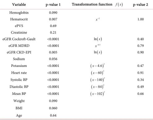
On the other hand, continuous variables were transformed in the context of logistic regression. For each continuous variable, a linearity test was performed using the method of restricted cubic splines with 3 knots [31]. A cubic spline re-stricted with 3 knots is composed of a linear component and a cubic component. Linearity testing is to test, under the univariable logistic model, the nullity of the coefficient associated with the cubic component. To do this, we used the likelih-ood ratio test. The results of linearity tests are given in Table 1 (p-value 1).
Table 1. Linearity tests and transformation of continuous variables.
Variable p-value 1 Transformation function f x ( ) p-value 2 Hemoglobin 0.090 Hematocrit 0.007 x−2 1.00 ePVS 0.69 Creatinine 0.21 eGFR Cockroft-Gault <0.0001 ln x( ) 0.40 eGFR MDRD <0.0001 x−0.5 0.79 eGFR CKD-EPI 0.005 ln x( ) 0.90 Sodium 0.056 Potassium <0.0001 ( )2 4.6 x − 0.47 Heart rate <0.0001 ( )2 60 x − 0.91 Systolic BP <0.0001 ( )2 140 x − 0.34 Diastolic BP <0.0001 ( )2 84 x − 0.49 Mean BP <0.0001 ( )2 102 x − 0.66 Weight 0.090 BMI 0.060 Age 0.64
DOI: 10.4236/am.2018.98065 966 Applied Mathematics
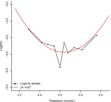
At 5% level, linearity was rejected for 9 of 16 continuous variables. For each of these 9 variables, we represented graphically the relationship between the logit (natural logarithm of the ratio probability of event/probability of non-event) and the variable. An example of graphical representation is given for potassium: we observe a quadratic relationship between the logit and the potassium (Figure 3). In agreement with the relationship observed, we applied a simple, monotonous or quadratic transformation function to each of the 9 variables. The transforma-tion functransforma-tion applied to each variable is given in Table 1.
For hematocrit and the three variables of eGFR, the relationship is clearly monotonous. So we considered some simple monotonic transformation func-tions as f x
( )
=xa with a ∈ − − −{
2, 1, 0.5,0.5,1,2}
or f x( )
=ln( )
x , then weretained for each variable the transformation for which the likelihood under un-ivariable logistic model was maximal (minimal p-value).
For other variables not checking linearity, namely potassium, the three blood pressure measures (systolic, diastolic and mean), and heart rate, the relationship between the logit and the variable was rather quadratic. We therefore applied a quadratic transformation function
(
X k− *)
2 with k∗ an optimal valuede-termined by maximizing likelihood under univariable logistic model. To com-pare, we also used the criterion of maximal AUC to determine an optimal value. These results are presented in Table 2. Notice that the optimal values deter-mined by the two methods are the same for systolic BP, diastolic BP and heart rate and are very close for potassium and mean BP.
Also note that the transformation applied to potassium allows to take into ac-count both hypokalemia and hyperkalemia, two different clinical situations pooled here that may increase the risk of death and/or hospitalization measured by the score.
DOI: 10.4236/am.2018.98065 967 Applied Mathematics Table 2. Quadratic transformations.
Variable “Raw” variable X likelihood for Criterion 1 Maximizing
(
X k− *)
2Criterion 2 Maximal AUC for
(
X k− *)
2AUC k* AUC k* AUC
Systolic BP 0.5818 140 0.5995 140 0.5995 Diastolic BP 0.5834 84 0.5970 84 0.5970 Mean BP 0.5915 102 0.6091 101 0.6094 Potassium 0.5312 4.6 0.5665 4.7 0.5676 Heart rate 0.6473 60 0.6521 60 0.6521
To verify that the transformation of the variables was good, a linearity test for each transformed variable was performed according to the previously detailed principle. All tests are not significant at the 5% level (see Table 1, p-value 2).
5.2. Ensemble Score
5.2.1. Ensemble Score by Logistic Regression
As a first step, we applied our methodology with the following parameters: use of a single classification rule, logistic regression (n =1 1),
draw of 1000 bootstrap samples (n =2 1000),
random selection of variables according to a single modality (n =3 1). Three modalities for the random selection of variables were defined: • 1st modality: random draw of m variables among 32,
• 2nd modality: random draw of m groups among 18, then one variable from
each drawn group,
• 3rd modality: random draw of m groups among 24, then one variable from
each drawn group.
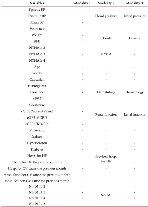
The groups of variables considered for each modality are presented in Table 3. For modalities 2 and 3, we formed groups of variables based on correlations be-tween variables. For the second modality, we gathered for example in the same group hemoglobin, hematocrit and ePVS because of their high correlations. For the third modality, the same groups were used, except for the two variables linked to hospitalization for HF, the four variables linked to the no. MI and the three variables related to the NYHA class, for which each binary variable was considered as a single group.
For each modality, an ensemble score was built for all possible values of m and the one that gave maximal AUC OOB was selected. In Table 4 are reported the results obtained for each modality with the optimal m. The best result was ob-tained for the third modality, with AUC OOB equal to 0.8634.
The ensemble score by logistic regression, denoted S x , obtained by aver-2
( )
aging the three ensemble scores that we constructed, gave slightly better results, with AUC OOB of 0.8649.
5.2.2. Ensemble Score by LDA for Mixed Data
The same methodology was used by simply replacing the classification rule (lo-gistic regression) by LDA for mixed data and keeping the same other settings.
DOI: 10.4236/am.2018.98065 968 Applied Mathematics Table 3. Composition of groups of variables.
Variables Modality 1 Modality 2 Modality 3 Systolic BP -
Blood pressure Blood pressure Diastolic BP - Mean BP - Heart rate - - - Weight - Obesity Obesity BMI - NYHA ≥ 2 - NYHA - NYHA ≥ 3 - - NYHA ≥ 4 - - Age - - - Gender - - - Caucasian - - - Hemoglobin - Hematology Hematology Hematocrit - ePVS - Creatinine -
Renal function Renal function eGFR Cockroft-Gault - eGFR MDRD - eGFR CKD-EPI - Potassium - - - Sodium - - - Hypertension - - - Diabetes - - -
Hosp. for HF - Previous hosp. for HF
- Hosp. for HF the previous month - - Hosp. for CV cause the previous month - - - Hosp. for other CV cause the previous month - - - Hosp. for non CV cause the previous month - - -
No. MI ≥ 2 - No. MI - No. MI ≥ 3 - - No. MI ≥ 4 - - No. MI ≥ 5 - -
Table 4. Results obtained by logistic regression.
Parameters AUC in resubstitution AUC OOB Modality 1 m = 19 0.8716 0.8616 Modality 2 m = 14 0.8688 0.8611 Modality 3 m = 8 0.8691 0.8634 Ensemble score 0.8728 0.8649
Again, for each modality, we searched the optimal m parameter. The obtained results are presented in Table 5.
As for logistic regression, the best results were obtained for the third modality, with AUC OOB equal to 0.8638.
DOI: 10.4236/am.2018.98065 969 Applied Mathematics Table 5. Results obtained by LDA for mixed data.
Parameters AUC in resubstitution AUC OOB Modality 1 m = 12 0.8679 0.8614
Modality 2 m = 5 0.8673 0.8631 Modality 3 m = 7 0.8690 0.8638 Ensemble score 0.8707 0.8654
The ensemble score by LDA, denoted S x , yielded better results with AUC 1
( )
OOB equal to 0.8654.
5.2.3. Ensemble Score Obtained by Synthesis of Logistic Regression and LDA
The final ensemble score denoted S x , obtained by synthesis of the two en-0
( )
semble scores S x and 1
( )
S x presented previously, provided the best re-2( )
sults with AUC equal to 0.8733 in resubstitution and 0.8667 in OOB.
This ensemble score corresponds to the one obtained by applying our metho-dology with the following parameters:
• two classification rules are used, logistic regression and LDA for mixed data (n =1 2),
• 1000 bootstrap samples are drawn (n =2 1000),
• m variables are randomly selected according to three modalities (n =3 3).
The scale of variation of the score function S x was reduced from 0 to 100 0
( )
according to the procedure described previously. We denote this “normalized” score S x .
( )
In Table 6, we present the “raw” and “standardized” coefficients associated with each of the variables in the score function S x and the “normalized” 0
( )
score function S x .
( )
5.2.4. Importance of Variables in the Score
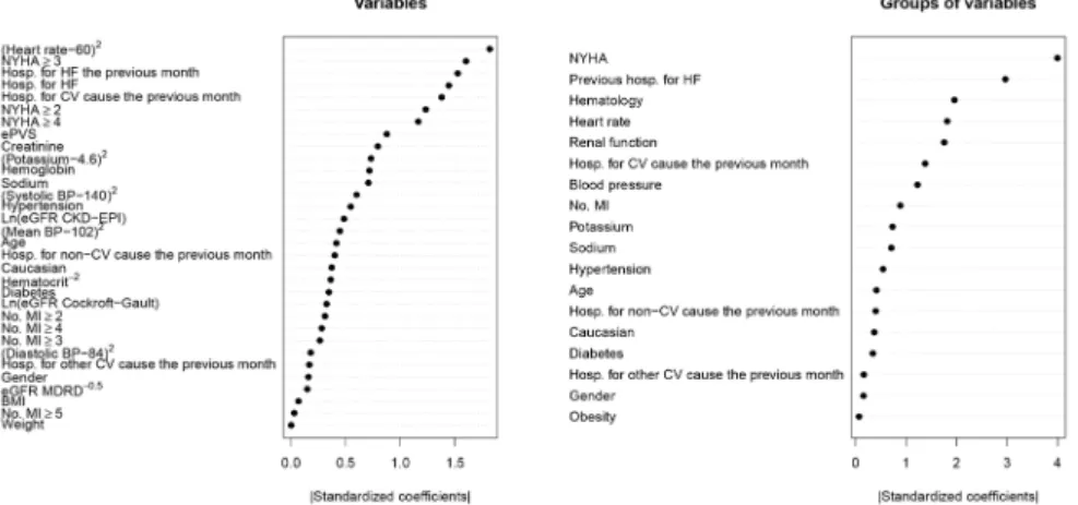
To have a global view of the importance of the variables in the “normalized” score, we represented on a graph the absolute value of standardized coefficient associated with each variable, from the largest value to the smallest (see Figure 4). Note that the most important variables are heart rate, NYHA class ≥ 3 and history of hospitalization for HF in the previous month. On the other hand, va-riables such as weight, no. MI ≥ 5 or BMI do not play a large part in the presence of others.
The same type of graph was made to represent the importance of the groups of variables in configuration 2 defined by the sum of the absolute values of the “standardized” coefficients associated with the variables of the group, from the largest sum to the smallest (see Figure 4). Note that the two most influential groups are “NYHA” (NYHA ≥ 2, NYHA ≥ 3 and NYHA ≥ 4) and “History of hospitalization for HF” (hospitalization for HF in the previous month and hos-pitalization for HF during life). Three important groups follow: “Hematology” (ePVS, hemoglobin, hematocrit), “Heart rate” and “Renal function” (creatinine and three formulas of eGFR). The least important groups of variables are “Obes-ity” (weight, BMI) and “Gender”.
DOI: 10.4236/am.2018.98065 970 Applied Mathematics Table 6. Ensemble score.
Variables Ensemble score S x 0( ) Ensemble score “normalized” S x ( )
coefficient Standardized coefficient coefficient Standardized coefficient Constant −0.210 −0.210 44.60 44.60 Hemoglobin −0.0580 −0.0871 −0.478 −0.717 Hematocrit−2 314.00 0.0442 2590.00 0.364 ePVS 0.131 0.107 1.07 0.877 Creatinine 0.00349 0.0964 0.0287 0.794 Ln (eGFR Cockroft-Gault) −0.0940 −0.0396 −0.774 −0.326 eGFR MDRD−0.5 −0.892 −0.0183 −7.34 −0.151 Ln(eGFR CKD-EPI) −0.175 −0.0590 −1.44 −0.486 Sodium −0.0232 −0.0861 −0.191 −0.709 (Potassium-4.6)2 0.301 0.0889 2.48 0.732 (Heart rate-60)2 0.000696 0.221 0.00572 1.82 (Systolic BP-140)2 0.000125 0.0729 0.00103 0.600 (Diastolic BP-84)2 0.0000985 0.0220 0.000810 0.181 (Mean BP-102)2 0.000201 0.0545 0.00165 0.448 Weight 0.0000258 0.000374 0.000212 0.00308 BMI 0.00196 0.00844 0.0161 0.0695 Age 0.00449 0.0506 0.0370 0.416 Caucasian −0.162 −0.0455 −1.33 −0.374 Male 0.0434 0.0195 0.357 0.161 Hypertension 0.136 0.0665 1.12 0.547 Diabetes 0.0904 0.0422 0.744 0.347 Hosp. for HF 0.549 0.175 4.52 1.44 Hosp. for HF the
previous month 1.53 0.185 12.60 1.52 Hosp. for CV cause the
previous month 0.403 0.168 3.31 1.38 Hosp. for non-CV cause
the previous month 0.361 0.0486 2.97 0.400 Hosp. for other CV cause
the previous month 0.104 0.0205 0.852 0.169 No. MI ≥ 2 0.0840 0.0377 0.692 0.310 No. MI ≥ 3 0.118 0.0323 0.973 0.266 No. MI ≥ 4 0.242 0.0342 1.99 0.281 No. MI ≥ 5 0.0443 0.00370 0.365 0.0304 NYHA ≥ 2 0.309 0.150 2.54 1.23 NYHA ≥ 3 0.612 0.194 5.04 1.60 NYHA ≥ 4 1.65 0.142 13.60 1.16
5.2.5. Risk Measure by an Odds-Ratio
We represented the variation of n0, n1, Se s ,
( )
1 Sp s−( )
, OR s and 1( )
( )
2
OR s according to the score s (Table 7). For score values s >49.1933, n1
is less than or equal to 30. Thus, beyond this threshold value 49.1933, OR1 is
no longer very reliable. We therefore defined as reliability interval of the OR1
DOI: 10.4236/am.2018.98065 971 Applied Mathematics Figure 4. Importance of variables and groups of variables.
Table 7. Variation of n , 0 n , 1 Se s ,
( )
1 Sp s−( )
, OR s and 1( )
OR s according to 2( )
the values of score s.
s n 0 n 1 Se s ( ) 1 Sp s− ( ) OR s 1( ) OR s 2( ) s* = 23.7094 4527 250 0.7918 0.2149 3.6844 3.6844 11.8489 19683 317 1.0000 0.9344 1.0702 1.0702 13.7320 17684 316 0.9968 0.8395 1.1874 1.1874 15.1105 15684 316 0.9968 0.7446 1.3388 1.3388 16.3630 13686 314 0.9905 0.6498 1.5245 1.5245 17.6044 11689 311 0.9811 0.5549 1.7679 1.7679 18.9050 9697 303 0.9558 0.4604 2.0762 2.0762 20.4525 7709 291 0.9180 0.3660 2.5081 2.5081 22.3007 5729 271 0.8549 0.2720 3.1428 3.1428 24.7670 3766 234 0.7382 0.1788 4.1278 4.1278 28.8573 1822 178 0.5615 0.0865 6.4884 6.4884 33.2656 872 128 0.4038 0.0414 9.7431 9.8363 38.2403 414 86 0.2713 0.0197 13.7706 13.7706 49.1933 70 30 0.0978 0.0033 29.4283 31.5217 55.1424 28 22 0.0694 0.0014 50.4112 50.4112 58.0352 14 16 0.0505 0.0007 70.8812 74.7575
We represented the variation of odds-ratio OR1 and OR2 in this reliability
interval (Figure 5). By reading the graph, for a patient with a score of 40 for example,
(
(
1| 40)
)
0 | 40
P Y S
P Y S
= >
= > is about 15 times higher than
(
)
(
10)
P Y P Y = = .6. Conclusions and Perspectives
In this article, we presented a new methodology for constructing a short-term event risk score in heart failure patients, based on an ensemble predictor built using two classification rules (logistic regression and LDA for mixed data), 1000 bootstrap samples and three modalities of random selection of variables. This score was normalized on a scale from 0 to 100. AUC OOB is equal to 0.8667. Note
DOI: 10.4236/am.2018.98065 972 Applied Mathematics Figure 5. Risk measure by an odds-ratio.
that an important variable such as potassium that does not appear in other scores (as SPIM risk score) is taken into account in this score.
Moreover, we defined a measure of the importance of each variable and each group of variables in the score and defined an event risk measure by an odds-ratio.
Due to the nature of the data available (data obtained from the EPHESUS study), we had to define the short term to 30 days in order to have enough pa-tients with HF event. It would be better to have data of papa-tients with shorter in-tervals, in order to have data the closest possible of an event and eventually im-prove the quality of the score. When such data will be available, it will be inter-esting to apply the same methodology to construct a new score.
Furthermore, we proved a property of linear discriminant analysis for mixed data.
Finally, this methodology can be adapted to the case of a data stream. Suppose that new data for heart failure patients arrives continuously. Data can be allo-cated to bootstrap samples using Poisson bootstrap [32]. The coefficients of each variable in each predictor based on logistic regression or binary linear discrimi-nant analysis can be updated online using a stochastic gradient algorithm. Such algorithms are presented in [33] for binary LDA and [34] for logistic regression; they use online standardized data in order to avoid a numerical explosion in the presence of extreme values. Thus the ensemble score obtained by averaging can be updated online. To the best of our knowledge, it is the first time that this problematics is studied in this context.
Acknowledgements
Results incorporated in this article received funding from the Investments for the Future program under grant agreement No ANR-15-RHU-0004.
DOI: 10.4236/am.2018.98065 973 Applied Mathematics
Conflicts of Interest
The authors declare no conflicts of interest regarding the publication of this paper.
References
[1] Levy, W.C., Mozaffarian, D., Linker, D.T., et al. (2006) The Seattle Heart Failure Model: Prediction of Survival in Heart Failure. Circulation, 113, 1424-1433.
https://doi.org/10.1161/CIRCULATIONAHA.105.584102
[2] Ketchum, E.S., Dickstein, K., Kjekshus, J., et al. (2014) The Seattle Post Myocardial Infarction Model (SPIM): Prediction of Mortality after Acute Myocardial Infarction with Left Ventricular Dysfunction. European Heart Journal: Acute Cardiovascular Care, 3, 46-55. https://doi.org/10.1177/2048872613502283
[3] Pitt, B., Remme, W., Zannad, F., et al. (2003) Eplerenone, a Selective Aldosterone Blocker, in Patients with Left Ventricular Dysfunction after Myocardial Infarction.
New England Journal of Medicine, 348, 1309-1321.
https://doi.org/10.1056/NEJMoa030207
[4] Duarte, K., Monnez, J.M., Albuisson, E., Pitt, B., Zannad, F. and Rossignol, P. (2015) Prognostic Value of Estimated Plasma Volume in Heart Failure. JACC:
Heart Failure, 3, 886-893. https://doi.org/10.1016/j.jchf.2015.06.014
[5] Cockcroft, D.W. and Gault, H. (1976) Prediction of Creatinine Clearance from Se-rum Creatinine. Nephron, 16, 31-41. https://doi.org/10.1159/000180580
[6] Levey, A.S., Coresh, J., Balk, E., et al. (2003) National Kidney Foundation Practice Guidelines for Chronic Kidney Disease: Evaluation, Classification, and Stratifica-tion. Annals of Internal Medicine, 139, 137-147.
https://doi.org/10.7326/0003-4819-139-2-200307150-00013
[7] Levey, A.S., Stevens, L.A., Schmid, C.H., et al. (2009) A New Equation to Estimate Glomerular Filtration Rate. Annals of Internal Medicine, 150, 604-612.
https://doi.org/10.7326/0003-4819-150-9-200905050-00006
[8] Lebart, L., Morineau, A. and Warwick, K. (1984) Multivariate Descriptive Statistical Analysis: Correspondence Analysis and Related Techniques for Large Matrices. Wiley, New York.
[9] Escofier, B. and Pagès, J. (1990) Multiple Factor Analysis. Computational Statistics and Data Analysis, 18, 121-140. https://doi.org/10.1016/0167-9473(94)90135-X
[10] Pagès, J. (2004) Analyse Factorielle de Données Mixtes. Revue de Statistique Appli-quée, 52, 93-111.
[11] Saporta, G. (1977) Une Méthode et un Programme d’Analyse Discriminante sur Variables Qualitatives. Analyse des Données et Informatique, Inria, 201-210. [12] Rotella, F. and Borne, P. (1995) Théorie et Pratique du Calcul Matriciel. Editions
Technip.
[13] Carroll, J.D. (1968) A Generalization of Canonical Correlation Analysis to Three or More Sets of Variables. Proceedings of the 76th Annual Convention of the Ameri-can Psychological Association, Washington DC, 227-228.
[14] Friedman, J.H. and Meulman, J.J. (2004) Clustering Objects on Subsets of Attributes (with Discussion). Journal of the Royal Statistical Society: Series B (Statistical Me-thodology), 66, 815-849. https://doi.org/10.1111/j.1467-9868.2004.02059.x
[15] Gower, J.C. (1971) A General Coefficient of Similarity and Some of its Properties.
Biometrics, 27, 857-871. https://doi.org/10.2307/2528823
DOI: 10.4236/am.2018.98065 974 Applied Mathematics Sélection de Variables. https://arxiv.org/pdf/1610.08203v2.pdf
[17] Hastie, T., Tibshirani, R. and Friedman, J. (2009) The Elements of Statistical Learn-ing. Springer, New York. https://doi.org/10.1007/978-0-387-84858-7
[18] Efron, B. and Tibshirani, R.J. (1994) An Introduction to the Bootstrap. CRC Press, Boca Raton.
[19] Breiman, L. (1996) Bagging Predictors. Machine Learning, 24, 123-140.
https://doi.org/10.1007/BF00058655
[20] In Lee, K. and Koval, J.J. (1997) Determination of the Best Significance Level in Forward Stepwise Logistic Regression. Communications in Statistics-Simulation and Computation, 26, 559-575. https://doi.org/10.1080/03610919708813397
[21] Wang, Q., Koval, J.J., Mills, C.A. and Lee, K.I.D. (2007) Determination of the Selec-tion Statistics and Best Significance Level in Backward Stepwise Logistic Regression.
Communications in Statistics-Simulation and Computation, 37, 62-72.
https://doi.org/10.1080/03610910701723625
[22] Bendel, R.B. and Afifi, A.A. (1977) Comparison of Stopping Rules in Forward “Stepwise” Regression. Journal of the American Statistical Association, 72, 46-53. [23] Tibshirani, R. (1996) Regression Shrinkage and Selection via the Lasso. Journal of
the Royal Statistical Society. Series B (Methodological), 58, 267-288.
http://www.jstor.org/stable/2346178
[24] Breiman, L. (2001) Random Forests. Machine Learning, 45, 5-35.
https://doi.org/10.1023/A:1010933404324
[25] Song, L., Langfelder, P. and Horvath, S. (2013) Random Generalized Linear Model: A Highly Accurate and Interpretable Ensemble Predictor. BMC Bioinformatics, 14, 5. https://doi.org/10.1186/1471-2105-14-5
[26] Akaike, H. (1998) Information Theory and an Extension of the Maximum Likelih-ood Principle. In: Parzen, E., Tanabe, K. and Kitagawa, G., Eds., Selected Papers of Hirotugu Akaike, Springer Series in Statistics (Perspectives in Statistics), Springer, New York, 199-213.
[27] Schwarz, G. (1978) Estimating the Dimension of a Model. The Annals of Statistics, 6, 461-464. https://doi.org/10.1214/aos/1176344136
[28] Tufféry, S. (2015) Modélisation Prédictive et Apprentissage Statistique avec R. Edi-tions Technip.
[29] Breiman, L. (1996) Out-of-Bag Estimation.
https://www.stat.berkeley.edu/~breiman/OOBestimation.pdf
[30] Dixon, W.J. (1960) Simplified Estimation from Censored Normal Samples. The Annals of Mathematical Statistics, 31, 385-391.
https://doi.org/10.1214/aoms/1177705900
[31] Royston, P. and Sauerbrei, W. (2007) Multivariable Modeling with Cubic Regres-sion Splines: A Principled Approach. Stata Journal, 7, 45-70.
[32] Oza, N.C. and Russell, S. (2001) Online Bagging and Boosting. Proceedings of Eighth International Workshop on Artificial Intelligence and Statistics, Key West, 4-7 January 2001, 105-112.
[33] Duarte, K., Monnez, J.M. and Albuisson, E. (2018) Sequential Linear Regression with Online Standardized Data. PLoS ONE, 13, e0191186.
https://doi.org/10.1371/journal.pone.0191186
[34] Monnez, J.M. (2018) Online Logistic Regression Process with Online Standardized Data.