Characterizing Shale Gas and Tight Oil Drilling and
A
Production Performance Variability
MAscSeETTSINSTITUTEby
MAY 26 2015
Justin
B.
Montgomery
LIBRARIES
B.S. Mechanical Engineering, Texas A&M University (2013)
Submitted to the Engineering Systems Division
in partial fulfillment of the requirements for the degree of
Master of Science in Technology and Policy
at the
MASSACHUSETTS INSTITUTE OF TECHNOLOGY
June 2015
@
Massachusetts Institute of Technology 2015. All rights reserved.
-- .4.It
Author...
Certified by...
Accepted by ...
Professor
Signature redacted
/1EngineeringSi
Systems Division
May 14, 2015
gnature redacted
Francis M. O'Sullivan
Director of Research, MIT Energy Initiative
Thesis Supervisor
... Signature redacted...
I
Dava J. Newman
of Aeronautics and Astrbnautics and Engineering Systems
Director, Technology and Policy Program
Characterizing Shale Gas and Tight Oil Drilling and Production
Performance Variability
by
Justin B. Montgomery
Submitted to the Engineering Systems Division on May 14, 2015, in partial fulfillment of the requirements for the degree of
Master of Science in Technology and Policy
Abstract
Shale gas and tight oil are energy resources of growing importance to the U.S. and the world. The combination of horizontal drilling and hydraulic fracturing has enabled economically fea-sible production from these resources, leading to a surge in domestic oil and gas production. This is providing an economic boon and reducing reliance on foreign sources of energy in the
U.S., but there are still a number of environmental, economic, and technical challenges that
must be overcome to unlock the resource's full potential.
One key challenge is understanding variability in individual well performance-in terms of both drilling time (a key driver of well cost) and well productivity-which has led to greater than anticipated economic risk associated with shale gas and tight oil development. Thus far, more reliable forecasting has remained elusive due to its prohibitive cost and the poorly understood nature of the resource. There is an opportunity to make use of available drilling and production data to improve the characterization of variability. For my analysis, I use publicly-available well production data and drilling reports from a development campaign.
In order to characterize variability, I use a combination of graphical, statistical, and data analytics methods. For well productivity, I use probability plots to demonstrate a univer-sality to the distribution shape, which can accurately be described as lognormal. Building on this distributional assumption, I demonstrate the utility of Bayesian statistical inference for improving estimates of the distribution parameters, which will allow companies to better anticipate resource variability and make better decisions under this uncertainty. For drilling,
I characterize variability in operations by using approximate string matching to compare
drilling activity sequences, leading to a metric for operational variability. Activity sequences become more similar over time, consistent with the notion of standardization. Finally, I investigate variability of drilling times as they progress along the learning curve, using prob-ability plots again. I find some indication of lognormality, with implications for how learning in drilling should be measured and predicted.
This thesis emphasizes the relevance of data analytics to characterizing performance variability across the spectrum in shale gas and tight oil. The findings also demonstrate the value of such an approach for identifying patterns of behavior, estimating future variability, and guiding development strategies.
Thesis Supervisor: Francis M. O'Sullivan
Acknowledgments
My advisor, Frank O'Sullivan, told me when I first arrived in Cambridge that I was not
going to have a "typical" research experience during my master's if I worked for him. This has proved more true than I could have imagined! Working with Frank has been a pleasure and I am grateful to him for always supporting my crazy ideas, challenging me, and making it easy to be excited about the work that I do every day. It is important to mention here that some parts of this thesis, especially Section 3.2.2, reflect not only my own analysis and interpretation but Frank's as well. I am grateful for the confidence he places in me as a researcher to collaborate closely with him on this work, and to build my own research efforts on shared insights. I have benefited tremendously from this relationship both as a researcher and as a person and I am excited to continue working together in the future!
I want to thank Accenture for financially supporting my analysis of drilling performance
variability. Being a part of the MIT-Accenture Business Analytics Consortium has been a unique and rewarding research experience. Additionally, the interactions I have had through-out this research with Melissa Stark, Brian Richards, John Tolle, Patrick Johnston, and Bob Palermo have been wonderful and I am grateful to them for their time, suggestions, and encouragement. While at MIT, I have been helped along the way by too many people to list here, but I especially want to thank Bob Kleinberg, Jessika Trancik, Gordon Kaufman, Youssef Marzouk, and Maite Pena-Alcaraz for their interest and help with my research. To all the people of the MIT Energy Initiative, thanks for making it a great environment to work in!
I also want to thank the Society of Petroleum Engineers for permission to base parts
of my thesis (specifically Sections 4.1 and 4.2) on material from a paper titled Measuring
Drilling Standardization Using Approximate String Matching that I presented at the SPE
ATCE 2014 conference in Amsterdam
I want to express my gratitude to some mentors, prior to my time at MIT, that have had
a profound impact on who I am professionally and personally: Mike Mayekar, Calvin Yao, Gregg Isenmann, Richard Malak, Ed Harris, Scott Austin (your memory and influence lives
on!), Kyle O'Leary, Charlie Hensel, Shane Aldrich, Craig Brown, and Michael Helms. This is not a list I make carelessly-I would not be where I am today if it was not for the time and attention invested in me by each of these individuals.
I have been surrounded by some truly incredible people in the last two years at MIT. I
have learned so much from my fellow TPP-ers2 and have thoroughly enjoyed being a part of this unique social experiment that places eccentric, social science-loving engineering students together. I can't imagine a more interesting and fun group of people to do a master's degree
with!
Speaking of social experiments, my home over the last two years has been a strange living arrangement called 'Murica. The transition from Texas to Massachusetts is a hard one in many ways and I would not have gotten through it without my roommates: Alex, Jacob, Chris, and John. They have been fantastic people to grow close with over this time and I know regardless of where we all end up, there will be a lifelong bond between us from this shared experience. Some of my fondest memories from these two years will be of sitting around our kitchen together in lawn chairs, drinking PBR, and watching the snow pile up outside. This is the graduate experience! But seriously, my mind has been stretched and my ideas challenged by all of our crazy conversations, and my understanding and appreciation of life is greater having known you guys.
I am incredibly fortunate that Cecilie came into my life a year ago. She has made
me a much happier person here and she continues to amaze me with how supportive and understanding she can be of me. Thank you so much for being by my side throughout this thesis and the last year.
Finally, I want to thank my family for their love and support. You all have taught me to enjoy hard work, be passionate about everything I do, and above all, to always have the courage to do things differently than everyone around me. This thesis is dedicated to you!
Now, enough with the sentimentalism. On with the show!
2
Contents
1 Setting the stage
1.1 P review . . . . 1.2 The growing importance of shale gas and tight oil . . .
1.3 Variability and economic risk . . . . 1.3.1 Under-appreciated variability and economic risk
1.3.2 Key drivers of resource economics . . . .
1.3.3 The need for new policies . . . .
1.4 Thesis question . . . . 1.4.1 M etrics . . . .
The background
2.1 Background on development process . . . . 2.1.1 Drilling the well . . . . 2.1.2 Completing the well . . . . 2.1.3 Unconventional oil and gas-a new set of d 2.2 Resource evaluation methods . . . .
2.2.1 Reservoir data collection . . . . 2.2.2 Reserve estimation in unconventionals . .
2.2.3 Statistical approach to resource evaluation
2.3 Learning in unconventional drilling . . . .
2.3.1 Empirical models of learning . . . .
2.3.2 Learning in organizations . . . .
evelopment
50 2.3.3 Procedural and performance variability and learning.
17 . . . . 17 . . . . 19 . . . . 22 . . . . 22 . . . . 23 . . . . 24 . . . . 25 . . . . 25 2 27 28 challenges 28 35 36 39 39 41 43 45 45 46
2.4 Benefits to characterizing the nature of performance variability . . . .
3 Characterizing production performance variability
3.1 Description of data and processing . . . . 3.1.1 Production data and initial processing . . . . 3.1.2 Transformation and normalization of production data . . . . . 3.2 Evaluating the shape of the productivity distribution with probability
3.2.1 Probability plots . . . .
3.2.2 Lognormality of productivity . . . .
3.2.3 Discussion of deviations at the ends . . . .
3.3 Bayesian inference of productivity distribution parameters . . . . 3.3.1 Background . . . .
3.3.2 Estimating the mean of a normal distribution . . . .
3.3.3 Estimating the mean for a ten square mile block of wells . . . 4 Characterizing drilling performance variability
4.1 Description of data and processing . . . . 4.1.1 Description of drilling report data . . . . 4.1.2 Conversion of drilling report data into operation sequences 4.2 Evaluating operational variability . . . . 4.2.1 Approximate string matching and operational dissimilarity 4.2.2 Demonstration of operational variability . . . . 4.2.3 Enabling automated and data-driven learning . . . . 4.3 Performance variability in the learning curve . . . . 4.3.1 The issue with learning curve noise . . . . 4.3.2 Characterizing the variability of noise . . . . 4.3.3 Implications of drilling performance variability . . . .
5 Closing remarks
5.1 Statistical importance of considering variability . . . . 5.2 Improving decision-making in unconventionals . . . .
51 55 56 56 57 58 59 61 66 74 plots 74 75 77 81 . . . . 83 . . . . 83 . . . . 84 . . . . 85 . . . . 85 . . . . 88 . . . . 91 . . . . 93 . . . . 93 . . . . 94 . . . . 96 111 111 113
5.3 Paving the rocky path forward for shale . . . . 116 119 127 A Tables
List of Figures
2-1 2-2 2-3 2-4 2-5 2-6 2-7Simplified schematic of onshore drilling rig. . . . .
A rig crew uses tools to break out drill pipe and then rack it back.
Diagram of top and bottom plugs for cementing casing. . . . . Slide and rotate drilling with a bent mud motor. . . . . Schematic of hydraulically-fractured shale gas system. . . . . Schematic geology of natural gas resources. . . . . Model of organizational learning and incomplete learning cycles .
. . . . . 29 . . . . . 31 32 . . . . . 34 . 36 . . . . . 37 49
3-1 Histograms showing distribution of well productivity in Barnett before and after normalization to standard score. . . . .
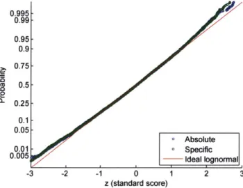
3-2 Probability plot comparing absolute and specific productivity in the Barnett
to an ideal lognormal distribution. . . . .
3-3 Probability plots comparing absolute and specific productivity of all plays to
an ideal lognormal distribution. . . . . 3-4 Probability plots comparing absolute and specific productivity of well ensem-bles in different Barnett counties to an ideal lognormal distribution. . . . . .
3-5 Probability plot comparing specific productivity of well ensembles in ten square mile blocks with 16 or more wells within Johnson county of the Barnett to an ideal lognormal distribution. . . . .
3-6 Probability plots comparing absolute and specific productivity of different vintages in the Barnett to an ideal lognormal distribution. . . . .
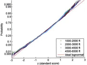
3-7 Probability plot comparing absolute productivity for Barnett well ensembles
categorized by perforation length to an ideal lognormal distribution. . . . . .
62 63 64 64 65 66 68
3-8 Probability plots comparing absolute and specific productivity of different
operating company well portfolios in Barnett counties to an ideal lognormal distribution . . . . 69 3-9 Probability plot comparing absolute productivity for Barnett wells to an ideal
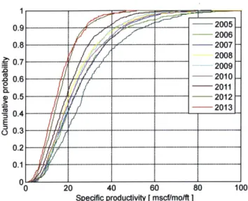
gam m a distribution. . . . . 70 3-10 Cumulative distribution function plot showing a general decline in specific
productivity by vintage in the Barnett. . . . . 71 3-11 Barnett shale play wells. Red indicates peak production in the top fifth
per-centile. Blue indicates peak production in the bottom fifth perper-centile. ... 72 3-12 Probability plot showing absolute productivity of Barnett wells compared to
an ideal lognormal distribution. Axes are linear scale of raw data without a log-transform ation. . . . . 73 3-13 Sum of squared error with different numbers of wells drilled for Bayesian
in-ference, maximum likelihood estimator, and county average (the prior knowl-edge) as a static estim ate. . . . . 80 4-1 Sequences of operation codes (raw data) mapped to Base64 characters. . . . 84
4-2 The initial comparison matrix is generated for the strings being compared. Many cells have been omitted here and are represented with ellipsis. . . . . . 86
4-3 Substring comparison steps and example comparison matrix. . . . . 99
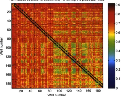
4-4 A color plot can be used to visualize the results of ASM for a series of wells. This color plot is similar to viewing a discretized surface plot from above. The plot here is not of actual data, and is intended only to be illustrative. . . . . 100 4-5 Color plot of normalized operational dissimilarity for drilling the production
h o le . . . 10 1 4-6 Operational variability captures the operational dissimilarity of a well relative
to the other most recently drilled wells (in this case using a scope of the ten previous w ells). . . . 102 4-7 A comparison of operational variability trends in different drilling modules. . 103 4-8 Normalized time for drilling the production hole . . . 104
4-9 Operational variability and time-based performance combined into one "bub-ble" plot with marker size based on operational variability. . . . 105 4-10 Operational variability can be used to provide additional insight into
differ-ences between drilling rig performance. . . . 106 4-11 Illustration of the variables used by Zangwill and Kantor
[155]
to evaluateeffectiveness. . . . 106 4-12 The power-law and exponential functions, the two most common forms of the
learning curve, were fitted to the waste times for wells in a drilling campaign using ordinary least squares nonlinear regression. . . . 107
4-13 Normal probability plots for residuals of power and exponential learning curve
fits... ... 107
4-14 Lognormal probability plots for residuals (with constant shift) of power and exponential learning curve fits. . . . 108 4-15 A plot of residuals in sequential order suggests homoscedasticity. . . . 108 4-16 Lognormal probability plots for residuals (with constant shift) of power and
exponential learning curve fits for first group (out of three groups) of wells. . 109
4-17 Lognormal probability plots for residuals (with constant shift) of power and exponential learning curve fits for second group (out of three groups) of wells. 109 4-18 Lognormal probability plots for residuals (with constant shift) of power and
exponential learning curve fits for third group (out of three groups) of wells. 110
B-1 Probability plot comparing absolute and specific productivity in the Marcellus to an ideal lognormal distribution. . . . 128 B-2 Probability plot comparing absolute and specific productivity in the Bakken
to an ideal lognormal distribution. . . . 128 B-3 Probability plot comparing absolute and specific productivity in the Eagle
Ford to an ideal lognormal distribution. . . . 129 B-4 Probability plot comparing absolute and specific productivity in the
B-5 Probability plot comparing absolute and specific productivity in the Barnett (based on first 12 months of production) to an ideal lognormal distribution. . 130
B-6 Probability plots comparing absolute and specific productivity of all plays (based on first 12 months of production) to an ideal lognormal distribution. . 130
B-7 Probability plots comparing absolute and specific productivity of well
ensem-bles in different Marcellus counties to an ideal lognormal distribution. . . . . 131 B-8 Probability plots comparing absolute and specific productivity of well
ensem-bles in different Bakken counties to an ideal lognormal distribution. . . . ..131 B-9 Probability plots comparing absolute and specific productivity of well
ensem-bles in different Eagle Ford counties to an ideal lognormal distribution. . . . 132
B-10 Probability plots comparing absolute and specific productivity of well
ensem-bles in different Haynesville counties to an ideal lognormal distribution. . . . 132
B-11 Probability plots comparing absolute and specific productivity of well ensem-bles in different Barnett counties (based on first 12 months of production) to an ideal lognormal distribution. . . . 133 B-12 Probability plots comparing absolute and specific productivity of different
vintages in the Marcellus to an ideal lognormal distribution. . . . . 133
B-13 Probability plots comparing absolute and specific productivity of different vintages in the Bakken to an ideal lognormal distribution. . . . . 134 B-14 Probability plots comparing absolute and specific productivity of different
vintages in the Eagle Ford to an ideal lognormal distribution . . . 134 B-15 Probability plots comparing absolute and specific productivity of different
vintages in the Haynesville to an ideal lognormal distribution. . . . 135 B-16 Probability plots comparing absolute and specific productivity of different
operating company well portfolios in Marcellus counties to an ideal lognormal distribution . . . 135
B-17 Probability plots comparing absolute and specific productivity of different
operating company well portfolios in Bakken counties to an ideal lognormal distribution . . . 136
B-18 Probability plots comparing absolute and specific productivity of different operating company well portfolios in Eagle Ford counties to an ideal lognormal distribution . . . 136 B-19 Probability plots comparing absolute and specific productivity of different
op-erating company well portfolios in Haynesville counties to an ideal lognormal distribution . . . . 137
B-20 Operational variability and time based performance for rig 1-drilling the pro-duction hole. . . . . 137
B-21 Operational variability and time based performance for rig 2-drilling the pro-duction hole. . . . . 138
B-22 Operational variability and time based performance for rig 3-drilling the pro-duction hole. . . . . 139
B-23 Operational variability and time based performance for rig 4-drilling the pro-duction hole. . . . . 140 B-24 Operational variability and time based performance for rig 5-drilling the
List of Tables
3.1 Summary statistics for specific productivity of counties in Barnett (Figure 3-4b). 62
3.2 Spread of productivity by vintage in Barnett (Figure 3-6). . . . . 67
3.3 Average number of nearby wells (within 0.564 mi. radius) for wells in the B arn ett. . . . . 71
A.1 Filtering criteria used for wells in each play. . . . . 120
A.2 General properties of the plays included in the characterization of productivity variability. . . . . 121
A.3 Summary statistics for specific productivity of counties in all plays . . . . 122
A.4 Spread of productivity by vintage in all plays. . . . . 123
A.5 Descriptions of operations included in Figure 4-1. . . . . 124
A.6 Description and examples of the edit operations within ASM and correspond-ing procedural changes they identify. . . . . 125
A.7 Potential edits, conditions restricting their use, and the method for finding the new value in each cell. . . . . 126
Chapter 1
Setting the
stage
1.1
Preview
In recent years, development of shale gas and tight oil resources has proceeded at a rapid pace. However, they have thus far been associated with widely varying development costs and initial production rates. These factors, combined with their rapid decline rates in production, make development of these resources an economically risky business, often only profitable at relatively high oil and gas prices. The nature of economic risk in these unconventional fields is still poorly understood, and in recent years this has led to a number of operating companies writing-down or selling shale assets due to highly variable, disappointing development results. There is a need to improve the process for characterizing uncertainty in these resources and ultimately forecasting the variability of their economic performance.
Alongside the development of these new and challenging resources, there is a growing interest in the answers that may be found in prolific field-generated data. Specialized tech-niques and expertise for extracting useful patterns from field data are still in their nascency though. This thesis aims to address some of the immediate questions about variability in shale gas and tight oil development, while also demonstrating the relevance of data analytics to this endeavor. I consider two distinct areas-well productivity and operations involved in drilling wells-which helps to illustrate the breadth of opportunity across many different aspects of shale gas and tight oil development.
production in North America and discuss some of the important implications and challenges associated with this. In this context, I discuss the general motivation behind my thesis question-how to characterize performance variability in these resources.
In Chapter 2, I provide additional background on shale gas and tight oil development and on characterizing and managing performance variability. I first describe the basic aspects of the development process, which are important to be cognizant of throughout this thesis. Then I discuss past philosophies and techniques for characterizing variability in conventionals and how these have been extended to unconventionals (a somewhat more general term that
I will use interchangeably with "shale gas and tight oil"). In many ways, unconventionals are
of a different nature than the conventional oil and gas resources dominant in the past. As
I discuss, they require a different set of development strategies due to the unique economic
and technical challenges associated with them, and these strategies are still evolving in the industry. Finally, I elaborate on the role of empirical models in both resource types and delve deeper into some of the motivations for improving our understanding of variability.
Chapter 3 introduces and defines a probability distribution of initial production rates in shale gas and tight oil-both between and within areas of a field. This new paradigm for pro-duction variability has implications for how operating companies approach the early stages of development, in which they acquire costly information to inform development campaign decision-making. To demonstrate the power of this variability characterization, I develop an application of Bayesian statistical inference that improves the ability to estimate acreage quality.
In Chapter 4, I investigate different aspects of performance variability, specifically the operational consistency and time-based performance of drilling unconventional wells. Or-ganizational learning leads to variation of drilling procedures and improvement of efficiency over time and the learning curve has thus far proved an important framework for under-standing performance improvement in the development process. It is important to develop additional performance indicators for abstract dimensions of the learning process. As an example, I turn to the phenomenon of "standardization," by which experimentation with drilling procedures over time yields standard operating procedures that are more uniform from one well to the next. I present a new technique for measuring standardization, which
also illustrates the importance of bringing analytics techniques from disparate disciplines to oilfield data, a hitherto under-utilized resource in the petroleum engineering discipline. I also discuss the challenges associated with measuring progress along the learning curve from an empirical perspective since literature in this area appears to be limited in its application to real world data and the natural variability that comes with it. I analyze the variability, or "noise," within the learning curve and discuss how consideration of this source of uncertainty
can improve current attempts to measure progress.
Chapter 5 serves as a concluding section to the thesis. I discuss the important elements of a more general framework for unconventional performance variability and I re-emphasize the importance of such considerations in light of the findings in this thesis. I include some general recommendations for the industry, public policymakers, and researchers based on the salient role of variability in managing the development of these resources.
This thesis answers one fairly abstract question but raises a number of other practical challenges that will require insight from a range of often silo-ed disciplines. Characterizing variability is really about charting a path toward promising ways to improve the management of variability. In this way, my thesis is not a conclusion of investigation but a jumping off point for the topic.
1.2
The growing importance of shale gas and tight oil
In the last ten years, the combination of horizontal drilling and hydraulic fracturing has pushed production from North American shale gas and tight oil plays to new levels and greatly expanded known domestic hydrocarbon resources [50, 126]. As a result, over the past decade US tight-oil production has increased six-fold while shale gas production has increased by more than a factor of four [50]. All of this has led many to predict a more hydrocarbon abundant future and to forecasts of the US becoming a net exporter of natural gas by 2018 and even a net oil exporter by 2030 [50, 36, 154, 87, 70].
The technical innovations that brought about this energy revolution about are in fact quite old. Horizontal drilling is a technique that allows drillers to gradually turn the direction of a well ninety degrees after drilling down thousands of feet vertically, and continue drilling
a well by a mile or more in the horizontal direction [152, 102]. Horizontal drilling was first accomplished in 1929 and became more widely used in the 1980s; its importance in shale gas development comes from drastically improving the economics of a well by accessing more of the resource, which is trapped within thin horizontal layers of rock formation [102].
Hydraulic fracturing is the other key enabler. It involves pumping large volumes of water mixed with chemicals and solids, at high pressures into a well to fracture rock within the formation, providing conduits for gas and oil to flow [152]. This reservoir stimulation technology has been used extensively since its first commercial application on a Kansas well in 1947 [102]. It is critical to shale gas production because of the extraordinarily low rock permeability (a measure of a rock's ability to allow fluid flow) found in these shale and "tight" (impermeable) sandstone formations [102]. It has been recognized for decades that prolific resources were present in these rocks but because of the extremely low rock permeability it was generally considered inaccessible (at least commercially) until recently [102]. Strong policy support for shale gas development combined with years of high domestic gas prices set the stage, but it was George Mitchell, a Texas entrepreneur who ignored industry naysayers and invested millions of dollars into years of experimentation in the Barnett shale of North Texas [139, 102, 42]. Eventually, his efforts paid off and he found a combination of horizontal drilling and hydraulic fracturing that made economic production of shale gas possible [102, 42]. Having already made a fortune, he abstained from patenting the process for developing these resources because he saw the potential good this knowledge could accomplish in the world as part of the public domain [42]. Thus was born one of the largest resource booms in recent history.
The economic benefits of these newly accessible resources are substantial, including lower energy prices for consumers, increased state revenues, reduced national energy imports, and even a shift toward some additional exporting of liquefied natural gas (LNG) and oil condensates [81, 115]. Furthermore, historically low natural gas prices in the United States are leading to a resurgence of manufacturing and associated jobs. Cheaper natural gas-derived feedstocks and low energy prices will increase domestic chemical and energy-intensive manufacturing by an estimated 20% over the next decade [37]. Additionally, oil prices have fallen by around half in the past year, driven in large part by surging U.S. oil production
from tight oil [43]. The windfall to consumers created by this leads to an estimated 0.2% boost in the world GDP for every 10% drop in the oil price [46]. Of course, the economic benefit is primarily for oil importing countries, while oil exporting nations like Venezuela and Russia are being fiscally pummeled by this price change, and find themselves with a diminished influence abroad [46, 9]. Low oil prices also present an excellent opportunity for fuel subsidies to be phased out, as they recently have been in Indonesia [9, 46, 45].
Another trend driven by the surge in shale gas production is a shift in electricity genera-tion in the U.S. from coal to natural gas [50]. Although natural gas emits half as much CO2
per unit of energy as coal, some of this climate benefit may be offset by fugitive methane emissions [86, 16]. There is currently a great deal of uncertainty about the amount of fugitive methane emissions emitted at the well site or at various stages within the natural gas supply chain [16]. Because of the large global warming potential of CH4 relative to CO2, this may
erode or even undermine the climate benefit for certain end uses [16, 47]. Still, many argue that natural gas has an important role to play as a "bridge" fuel, easing the transition away from coal and complementing the intermittent nature of solar and wind energy due to its flexibility as a generation source [86, 136].
The shift from coal to natural gas will also lead to a reduction in mercury, NOR, SO2,
black carbon, CO, and particulates emitted from the power sector, thereby reducing as-sociated illnesses and deaths and generally improving public health [86]. However, there are substantial concerns regarding local environmental risks associated with the extraction process including potential groundwater and surface-water contamination, local air quality issues, and induced seismicity from wastewater disposal in injection wells [83, 149, 72, 156]. It is essential that industry, researchers, and policymakers continue to work toward a better understanding and management of these risks through improved technologies and regulation. In contrast to the growing role of shale gas and tight oil production in the U.S., efforts to build a similar unconventional boom elsewhere have so far foundered [24, 129]. Nevertheless, this resource has been touted as a world game-changer economically, environmentally, and geopolitically, given the widespread unconventional basins of the world (such as in China, Poland, and Argentina) and the world's insatiable appetite for inexpensive and secure sources of energy [44, 106, 49, 84].
1.3
Variability and economic risk
1.3.1
Under-appreciated variability and economic risk
In spite of this hubris about the resource potential, concerns abound regarding the long-term economic viability of shale gas and tight oil development [144, 100, 74, 80, 27]. There is now growing concern about the variability of well productivity and rapid production decline rates, which necessitate huge capital-expenditure on drilling campaigns to maintain rates of production [100, 80, 27]. It has recently been estimated that as many as 40% of unconventional wells in the U.S. are uneconomical due to variability of drilling, completion practices, and reservoir characteristics
[54].
There is a wide range of production variability in fields, persisting even in recent years with supposedly "mature" development practices[541.
These production challenges have contributed to some major operating companies writing down the value of unconventional assets and even exiting from major plays [75, 145, 123]. Internationally, there have also been signs of tapering expectations, including an exodus of energy companies from Poland, and China halving its shale gas production targets for 2020 [24, 129]. The recent plummet in oil prices is casting additional doubts on the extent to which industry will continue to invest in developing these resources
[1].
Despite the mounting evidence that economic risk in shale gas and tight oil development has thus far been under-appreciated, the nature of performance variability is still poorly understood. Increasing economic pressure from low oil and gas prices means it will be necessary to improve forecasting and decision-making in fields early on, taking into account this performance variability and making greater use of available data [55, 71]. Deterministic forecasting of expected field performance (even if this is scaled up and down to provide a spread of economic outcomes) is misleading because of important statistical features like distribution skewness [67]. More transparent models of field performance variability are also needed to aid decision-making in light of nuances like physical production constraints (i.e. shared pipeline capacity) and the non-linearity of value with shifts in variables [67]. Decision-making in unconventional development campaigns should be guided not only by traditional engineering, geological, and economic assessments but also by simple, short-term predictive performance metrics that allow visualization and description of variability patterns within
large datasets
[147].
1.3.2
Key drivers of resource economics
A major driver in the economics of unconventional wells is development cost, including the
cost of drilling and completions (hydraulic fracturing) [35]. Well construction is the highest cost in onshore oil and gas development ( 70-90% of overall costs) and is one of the main
areas for onshore operating companies to compete with each other on extracting petroleum resources at the lowest per-unit cost [89]. The horizontal wells necessary in unconventional fields are much more expensive to drill than vertical wells, in part because the specialized drilling equipment and techniques required present numerous technical challenges and signif-icant outcome variability [89]. In fact, well cost is lognormally distributed and unpredictable due in large part to the costly unplanned activity needed to address equipment failures, geological uncertainties, and inconsistency of implementation in drilling operations [89]. Be-tween 2007 and 2012, the average cost to drill and complete a well in the Haynesville shale play was $9.8 million with a standard deviation of $2.0 million [89]. Average drilling costs per well were around 45% of these costs but the unitized risk, or coefficient of variation, was higher for drilling than completions (0.3, compared with 0.24) [89]. The variation in completions cost is also more likely than the variation in drilling costs to have been planned and expected by operators.
Learning is critical for improving the efficiency of well construction in shale gas and tight oil development campaigns. An analysis of over 200 horizontal wells drilled in the Eagle Ford shale play by 31 different operators between 2008 and early 2011 found a trend toward decreased drilling days per footage over time, but there was large variation in total drilling days for similar well depths and and trajectories [62]. This suggests that greater consistency of implementation may lead to even larger improvements [62]. Indeed, a focus on greater consistency of learning efforts led Shell to work toward improving the organizational structure for capturing and sharing drilling best practices, allegedly reducing well delivery times by a factor of three in a relatively short time [148]. The specific levers behind the "learning curve"-which describes increased efficiency with increased experience-are not clear, but the process generally involves experimentation to adapt to local conditions, and standardization
of the drilling approach [148]. The ability to spread learning from one rig or field to another and to quantify high-level metrics of performance improvement and consistency are critical steps toward effectively managing this temporal reduction in drilling costs [17, 148].
Another major source of uncertainty about economic success is the production profile of a well. The initial production rate and the rate at which the production declines from the peak rate achieved during the first few months of the well's life are highly variable and challenging to predict [35]. As much as two-thirds of the uncertainty about a well's net present value may be related to the production profile [68]. A well that has begun producing still has uncertainty about the future rate of decline in production, but is also a significant source of information about the area in which it was drilled. In addition to any well log data and core samples collected during drilling, there is immediately available information in the form of production data, which can be used to assess the acreage quality and evaluate completions techniques. Production from an early well can be used to support the critical decision of whether to continue drilling additional wells or abandon an area (the "go/no-go decision") [68]. However, even wells drilled from the same well pad may have widely different results, and the "data point" the well provides is useless for decision making if it is not considered more broadly within the potential variability of the area
[116].
1.3.3
The need for new policies
The current shortcomings at understanding and managing variability may partly stem from an inability to adapt a "conventional mindset" for oil and gas development to the new chal-lenges presented by unconventionals
[55].
Economic success in shale plays requires a combi-nation of efficiency (low development costs) and effectiveness (high well productivity) [54]. Many in industry have focused primarily on the need for greater efficiency by advocating a "factory approach" to development [53]. This philosophy may have some merits, but taken alone, it gives inadequate consideration to the consistency of the product. A fantastically efficient factory that is unpredictable and delivers widely varying results should hardly be an aspiration for the oil and gas industry. Indeed, in this sustained downturn in oil prices, ques-tions have been raised as to whether a factory-inspired approach to drilling a large number of wells at the lowest cost possible is really a better strategy than focusing on achieving fewer,more-productive wells
[55].
Part of this shift will require a replacement of unsystematic field experimentation with thorough analysis and planning [55].The continued success of unconventional resource development within the U.S. and the spread of development to other parts of the world depends in large part on the ability to characterize, forecast, and manage the variability associated with these resources. Further development of this capability will support reliable assessments of a field's economics early on, more optimal planning, and faster learning during a field development campaign.
1.4
Thesis question
Concern about this important and poorly understood dimension of shale gas and tight oil development leads me to my thesis question: How should an operating company characterize
the variability of drilling and production performance of wells using existing field data? There
is a substantial opportunity to develop approaches that makes use of "free" unused field data to supplement and guide other more costly approaches, improve forecasting early in a development campaign, and provide a foundation for more advanced understandings of uncertainty and techniques for mitigation. This thesis makes an important contribution to this area by identifying some key patterns of variability and providing tools for assessing them.
1.4.1 Metrics
There are many ways in which this topic could be taken on. At this point though, I should define clearly the performance metrics I use, with some justification for each. These metrics attempt to address some important aspects discussed in the previous section, while also making use of the data that I had access to.
For production performance, I focus on the peak production rate of a well, which typi-cally occurs within the first few months of production. Peak production is correlated with, and is commonly used as a proxy, for early-life production, and to a lesser degree, lifetime production [147, 125, 100]. Due to the rapid decline rates in production and the discounting of revenue from future production, early life production is critical to shale gas and tight oil
resource economics' [147]. Initial production rates may be more indicative of the quality of the stimulated fracture network created than the underlying reservoir quality, but it's economic importance is still key. I have also considered an alternative metric for production performance-production in the first 12 months, which is likely more reflective of the under-lying reservoir quality-and Appendix B includes a handful of figures extending my analysis to this.
For drilling performance I rely first upon drilling time (or, in some cases, time per footage of well drilled). More broadly, I am interested in variability of cost, but drilling time is a particularly important and substantial source of variability for this. Rig rental is the largest component of drilling costs (followed by labor, which could also be thought of as having a "daily" cost) [89]. Haynesville rigs between 2008 and 2012 had a base day-rate of $12,500-$22,000, excluding fuel and add-on costs2 [89]. The only larger component of an overall well's costs is stimulation and sand control (associated with completions, not drilling) but these are static material inputs less susceptible to change over time or unpredictability. Reduction of these inputs might also negatively impact production whereas a well can be drilled just as effectively in different amounts of time depending on the efficiency of operations. Analysis of drilling time also allows me to investigate learning effects. Time is considered a better proxy of learning than directly measuring cost since it is not confounded by changing rig or equipment day-rates [17, 89].
Finally, I develop an additional metric for drilling performance that addresses the con-sistency of drilling procedures from one well to the next. I call this "operational variability" and use it to detect procedural "standardization" which takes place during the learning pro-cess. Additional work will be needed to realize the full potential for field deployment of this metric, but nevertheless it provides an interesting example of how analytics can be used to visualize hidden behaviors in a sociotechnical system and allows for immediate insights into how the drilling process changes over time in a field development campaign.
'Production flow rates in wells fall by around 50% in the first year, and substantially more after three years-by some estimates, to as low as 5-20% of the peak production rate (142, 74].
2
The "effective" day rate for drilling (including all drilling costs divided by days of drilling) ranges from
Chapter 2
The background
Unconventionals present the oil and gas sector with a fundamentally different type of eco-nomic risk than it is used to dealing with [74, 80, 27]. The high degree, and distribution of well-to-well production variability means companies are exposing themselves to appreciable economic risk each time they roll the die by drilling a well, even after many nearby wells have been drilled. This contrasts with economic risk in conventional oil and gas development, which is driven more by uncertainty about the size and presence of hydrocarbon accumu-lations and can be mitigated by geological data collection and reservoir simulation carried out during exploration [131, 1431. Characterizing the distribution of well productivity in shale gas and tight oil fields is critical to better understanding the production variability-a major factor in the economic risk associated with these resources [116].
Furthermore, observed variability of drilling operations and time-based performance sug-gests companies are often investing significantly more capital over the course of a field's development than would be necessary with greater operational consistency and faster orga-nizational learning [148, 89]. Better understanding the nature of the variability present in the drilling process will improve the ability to forecast future drilling costs in a field, pro-mote best practices and measure learning within a development campaign, leading to greater efficiency and effectiveness at earlier stages of development.
This chapter reviews some relevant literature to the issues of performance variability facing developers of unconventional assets in North America today. Because of the broad, systems perspective of my thesis, a breadth of interrelated topics are involved, and in
re-viewing them here I can only skim the surface of these prolific areas of existing knowledge and ongoing research. As in the rest of this thesis, precise causal relationships and full ap-preciation of the many involved nuances is of less concern than framing the bigger picture question, of how generally to think about the issue of variability in production and drilling performance in unconventionals and develop new techniques that can be incorporated into the overall development process to improve its management.
2.1
Background on development process
In this section I provide a basic overview of the operations for drilling and completing a massively hydraulic-fractured horizontal well typical in North American shale oil and gas fields. I then discuss some of the differences between the geology and development strategy of unconventionals and conventionals and the challenge that this is presenting to the oil and gas industry.
2.1.1
Drilling the well
An excellent reference on the process of drilling a well is A Primer of Oilwell Drilling by Bommer [13]. The following description is drawn from this source, unless otherwise noted, and should be referred to for greater clarity and additional illustrations.
The actors - An operating company owns, manages, and engineers the wells being
developed. The fieldwork is carried out by drilling and service contractors.
Site preparation - The well location is determined based on a variety of legal and
eco-nomic factors including the need to obtain a lease to drill there. If other wells have been drilled in the area, the placement of a well may be informed by knowledge obtained from them. In any case, geologists and geophysicists will generally suggest areas they think likely to be productive based on promising expected geology from available data. Prior to bringing the drilling rig on location, the drilling site is cleared and flattened if necessary. A reserve pit is dug to store waste drilling fluids. Other earthen pits may also be dug alongside to store water and rock cuttings. The primary drilling fluid, "mud," is generally stored in metal tanks to maintain quality. A small, secondary rig might at this point drill any nearby holes
necessary for temporarily storing drill pipes. Additionally, in some cases this smaller rig might "spud," or drill the initial hole which is wide but shallow. This conductor hole is lined with casing and cemented in place. Alternatively, this last step of spudding the well might be done by the main rig once it is on site.
Rig move (from previous well) and rig up - The disassembled rig is moved to the well
site on trucks, or if it is a "skid" rig, it is towed to the site. During rig up, the process varies based on rig type. For instance a "slingshot" rig can be elevated using hydraulic pistons. The "drawworks," which hoists or lowers a cable called a "drilling line," and other substructure equipment are set up and the mast or derrick is raised into position. This system will be used to raise and lower everything in and out of the wellbore [152]. Additional equipment is "rigged up," including electric generators, steel mud tanks, pumps, stairways and walkways. Living quarters are brought on site along with drill pipe, pipe racks and other drilling equipment.
A metal building called a "doghouse" is set up next to the rig floor for the driller and crew
to use as an office. A representative but highly simplified schematic of an onshore drilling rig is shown in Figure 2-1.
Equ~pmri
rMS4Cuffingp
Figure 2-1: Simplified schematic of onshore drilling rig. Source: Tidal Petroleum
Drilling the surface hole - Once rigging up is complete, the well is spudded and the
The surface hole is then drilled to a depth of a few thousand feet typically, using a large diameter surface drill bit "made up" to a "bit sub." As the hole is drilled, "drill collar" is added above the bit sub. This creates the "bottom hole assembly" (BHA) used to drill the well, which is the bottom portion of the "drill string," or column of connected drill pipe and equipment at any given time. Once the BHA is made up, drill pipe is added to lengthen the drill string and allow the bit to reach the bottom of the deepening wellbore. To make
up (i.e. connect) the segments of drill pipe, "roughnecks," or fieldworkers, guide suspended
drill pipe into place at the top of the drill string once it is flush with the rig floor. They then use tongs or specialized equipment to apply torque to the drill pipe and tighten the screw threads between pipes. Drive systems vary but they all allow rotation of the entire drill string [152]. It is this rotation, referred to as "rotate drilling," that is generally used to turn the bit and crush rock at the bottom of the wellbore. Mud is circulated through the drill string and back up the annulus of the hole in order to return drill cuttings and to maintain bottomhole pressure [152].
Tripping out - Once the planned depth for the surface hole is reached, the drill pipe is
"tripped out" and stored. In order to trip out pipe, the drill string is pulled out gradually to expose a stand of pipe. Pipe is then "broken out" using equipment to rotate it and spin out the threads (Figure 2-2a). The pipe is then racked back (Figure 2-2b).
Running and cementing surface casing - Next, metal casing will be put in place and
cemented to isolate the surface hole from the surrounding rock and surface water. The casing joints are added in a similar manner to that of drill pipe until the casing reaches the bottom of the surface hole. A cementing company brings cement-pumping equipment to the site and mixes the cement slurry. The cement is pumped into a cementing head that is attached to the top joint of casing. A "bottom plug" is dropped from the head just before the cement in order to keep mud in the wellbore from contaminating the cement slurry and to push the mud on through and back up the annulus. When the plug reaches the bottom of the casing, it sits in a "float collar" that is in place there. This causes a membrane to be broken and cement flows out of the bottom of the casing and fills the annulus space around the casing from the bottom up. When the last of the cement is pumped, the "top plug" is dropped to separate the cement from the displacement fluid, which is pumped after it to fill the inside
(a) Source: Troy Fleece Photography
(b) Source: OSHA
Figure 2-2: A rig crew uses tools to break out drill pipe and then rack it back. of the casing and displace the cement.. A pressure jump indicates that the top plug has "bumped" the bottom plug and the cement has filled the annulus of the casing, ending the cement job (Figure 2-3).
A period of a few hours follows for waiting on cement. After this, the wellhead can be
installed and the blow-out preventer (BOP) placed, or more formally, "nippled up." Pressure testing of the BOP stack, wellhead, and well is carried out before further drilling can occur.
Tripping in and drilling out the shoe - The BHA for the next section of the well is picked
up first and the bit is returned to the bottom of the hole by adding stands of pipe back to the drill string as it is lowered. Once the bit reaches the bottom of the surface casing, the bit drills out the equipment and cement at the bottom then starts making new hole. Before proceeding to drilling the next section of hole, the casing and cement job is pressure tested.
Constructing other sections of the well and downhole maintenance - The well may be
designed to have two, three, or even four well sections (the surface hole is the first as the conductor hole is not generally counted). This is generally determined by drilling engineering calculations taking into account the target depth and pressure regime. The other sections are drilled, cased, and cemented in essentially the same manner as the surface hole. Casing for
Top plug
Solid core
Bottom plug Rupture disk
Hollow core
Figure 2-3: Diagram of top and bottom plugs for cementing casing. Source: Schlumberger these additional well sections may be run all the way to the surface or it may be suspended from a hanger and act as a liner beyond the first string of casing. During drilling of any of the sections, additional round trips may (and likely will) be required because of equipment failures or a need to change out the bit or BHA to achieve different drilling parameters. If a tool or other item is lost downhole it may be retrieved using "fishing equipment." Small items may also be drilled using "junk mills" if they are not retrieved. In addition to these downhole issues, problems with procedures or equipment at the surface may lead to nonproductive time
(NPT), which may be interspersed throughout the overall process and is a frequent source of
wasted time in the drilling process. There are many other activities that may be carried out throughout the drilling process, either to recover from unintended outcomes, or to attempt to preempt them. An example of this is pumping through the well different mixtures of drilling fluids, in precise volumes and densities, and sometimes containing solids1 in order
to control the wells behavior. The variability of these procedures from one well to the next will be relevant in the later discussion of operational variability in Chapter 4.
Drilling the curve section - Directional drilling in shale wells can be accomplished using
either "slide drilling" with a "mud motor" or "rotary steerable assemblies." With slide drilling the BHA contains a section of bent housing that orients the bit at a small angle (Figure 2-4). The bit can then be pointed by holding the drill string steady and turning the bit
'Peanut shells may even be used as "lost-circulation material" to prevent loss of drilling fluids through the wellbore sides [134]!
by pumping mud through the hydraulically powered downhole mud motor. A "measurement
while drilling" (MWD) tool placed higher up in the BHA detects the direction of the hole and sends pressure pulses back to the surface to relay the information. Once the desired direction is achieved the directional BHA can be rotated conventionally with the drill string and the current direction will be maintained because the bend in the mud motor has no preferred direction (Figure 2-4). This is much faster than slide drilling. If a rotary steerable assembly is used instead of slide drilling then the wellbore path is programmed into a computer in the assembly. The computer steers the drill bit while the drill string is being rotated allowing for more rapidly drilled curves.
Sliding Rotating
Figure 2-4: Slide and rotate drilling with a bent mud motor. Source: Oil & Gas Journal
Drilling the lateral section - In the lateral section a different BHA with a smaller bend
angle may be used or the curve assembly may remain in place if the bend angle is not too large. The lateral section is drilled primarily by rotating the drill string. If the BHA "walks" and veers from the planned path or if the target zone is changed then some slide drilling may be required to change the wellbore direction.
Rig down/skid/slide - After the well total depth (TD) has been reached and the
pro-duction casing installed the well is fully drilled. The rig is either disassembled and trucked to another site or skidded to a location nearby. For multi-well pads, the rig may be on slides that allow it to be quickly shifted in order to drill other wells alongside before it is removed from the site.
that are intended to be homogeneous and standardized to promote efficiency. Almost every step described here has either some caveat, slightly different alternative approach, or more detailed set of optional and required procedures that I have neglected to mention here in the interest of brevity. The process is also not as linear as I have described it here. Many of these procedures are in reality mixed and matched in various orders, particularly when the oper-ating company and crew engaged are less familiar with the field being developed (i.e. early in a drilling campaign). Variations may enter the process due to unforeseen conditions (and the need to mitigate them), differences in opinions and 'styles' of drilling engineers, com-pany men and superintendents (field managers), planned experimentation with procedures to determine bast practices for the field, and inconsistency of the field crew at implementing the procedures. Chapter 4 will consider how to measure this operational variability and the variability in time-based performance improvements as an operating company and crew "learns" the best way to implement consistent wells in a field. Some further background on learning in oil and gas drilling will be provided in Section 2.3.
2.1.2
Completing the well
I will not go into as great of detail describing the process of completing, and hydraulically
fracturing the well, as I have for the drilling operations of a well because the step-by-step procedure is of less interest to this thesis.
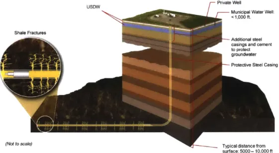
Completing the well includes casing and cementing the well2, perforating the horizontal
section of well with shape charges from a perforation gun, installing production equipment (production tubing and production wellhead), and stimulating the reservoir with hydraulic fracturing, or "fracking" (Figure 2-5) [13]. Hydraulic fracturing is essential to production of oil and gas from extremely low permeability unconventional reservoirs. Hydraulic fracturing involves pumping between 2 and 20 million gallons of water, mixed with specialized chemicals, and proppants such as sand or other solids into the well, and out of the perforations [83]. The volume and pressure (10,000-20,000 psi typically) is sufficient to fracture the rock around the well and drive the propagation of these cracks out into the rock formation to provide a flow path for fluids trapped in the shale reservoir [83]. The solid proppant is wedged into the
2
![Figure 2-7: Model of organizational learning and incomplete learning cycles. Adapted from March and Olsen [107]](https://thumb-eu.123doks.com/thumbv2/123doknet/14268918.490156/49.918.227.650.418.667/figure-model-organizational-learning-incomplete-learning-cycles-adapted.webp)