READ THESE TERMS AND CONDITIONS CAREFULLY BEFORE USING THIS WEBSITE. https://nrc-publications.canada.ca/eng/copyright
Vous avez des questions? Nous pouvons vous aider. Pour communiquer directement avec un auteur, consultez la première page de la revue dans laquelle son article a été publié afin de trouver ses coordonnées. Si vous n’arrivez pas à les repérer, communiquez avec nous à PublicationsArchive-ArchivesPublications@nrc-cnrc.gc.ca.
Questions? Contact the NRC Publications Archive team at
PublicationsArchive-ArchivesPublications@nrc-cnrc.gc.ca. If you wish to email the authors directly, please see the first page of the publication for their contact information.
NRC Publications Archive
Archives des publications du CNRC
This publication could be one of several versions: author’s original, accepted manuscript or the publisher’s version. / La version de cette publication peut être l’une des suivantes : la version prépublication de l’auteur, la version acceptée du manuscrit ou la version de l’éditeur.
Access and use of this website and the material on it are subject to the Terms and Conditions set forth at
Calibration of an Anamorphic Laser Based 3-D Range Sensor
Blais, François; Beraldin, Jean-Angelo
https://publications-cnrc.canada.ca/fra/droits
L’accès à ce site Web et l’utilisation de son contenu sont assujettis aux conditions présentées dans le site LISEZ CES CONDITIONS ATTENTIVEMENT AVANT D’UTILISER CE SITE WEB.
NRC Publications Record / Notice d'Archives des publications de CNRC:
https://nrc-publications.canada.ca/eng/view/object/?id=fa5ebc5a-4c16-44c2-9850-5ab168736bb0 https://publications-cnrc.canada.ca/fra/voir/objet/?id=fa5ebc5a-4c16-44c2-9850-5ab168736bb0
National Research Council Canada Institute for Information Technology Conseil national de recherches Canada Institut de technologie de l'information
Calibration of an Anamorphic Laser Based
3-D Range Sensor *
Blais, F., and Beraldin, J.-A.
July 1997
* published in theSPIE Proceedings, Videometrics V. San-Diego, California, USA. July 27 -1 August 1997. Volume 3174. pp. 113-122. NRC 40216.
Copyright 1997 by
National Research Council of Canada
Permission is granted to quote short excerpts and to reproduce figures and tables from this report, provided that the source of such material is fully acknowledged.
Calibration of an Anamorphic Laser Based 3-D Range Sensor*
François Blais, J.-Angelo Beraldin
Institute for Information Technology
National Research Council Canada
Ottawa, Ontario, Canada, K1A - 0R6
blais@iit.nrc.ca
beraldin@iit.nrc.ca
ABSTRACT
This paper describes the parameters and method used to calibrate an anamorphic lens specially designed for a 3-D triangulation based laser range sensor. It expands the more “conventional” spherical lens calibration technique that has been developed in photogrammetry to include the extra distortions introduced by the strong astigmatism and by the different optical principal planes of the lens of the anamorphic design. Experimental results using a prototype of the lens for the Biris range sensor are presented.
Keywords: Anamorphic, calibration, range sensors, lens model, photogrammetry.
2.
INTRODUCTION
A trend in cinematography that has once been very popular was to provide the audience with a wide field of view screen. Of course the technique known as “CinemaScope," could have been accomplished using a wide film (e.g., 70 mm rather than the conventional 35 mm). However it was found to be more economical and more convenient to photograph and project using the more conventional and widely used 35 mm film and an anamorphic optical lens system.1,2
An anamorphic optical system is one that has a different power along mutually perpendicular meridians. Such devices usually make use of either cylindrical lenses or prisms. In the CinemaScope, a 2× anamorphic afocal cylindrical attachment is placed in front of the primary spherical lens. This attachment has no effect in the vertical dimension but compresses the horizontal image on the film. Projection is accomplished in the same manner; an afocal cylinder attachment is placed in front of a standard projection lens and “expands” the compressed image.
Diodes laser optics is another example of an anamorphic optical system. Diode lasers have a divergent asymmetric output due to diffraction effects in the asymmetric gain region of the laser cavity. Prisms and cylindrical corrections optics are used to project a circular laser beam instead of the usual elliptical beam.
In the following sections, the advantages of using an anamorphic lens design with a 3-D laser based range sensor are discussed. The benefits of increasing the field of view of the sensor while preserving the range accuracy of the system are presented. The method used to calibrate this anamorphic design is then discussed and experimental results are shown using the NRC’s Biris range sensor. Although the discussion is mainly focused on the NRC’s technology, it is directly applicable to most triangulation based methods.
* NRC 40216
3.
RANGE TRIANGULATION
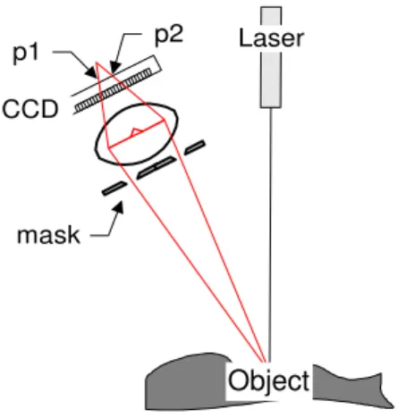
The Biris range sensor is a combined triangulation and focus based technique. The range information is gathered by projecting a laser plane on an object and imaging the projected laser line using a dual aperture mask inserted inside the camera lens. The combined Biris-plane of light principle is depicted in Figure 1.
Because of the two aperture mask and the defocusing of the image, two distinct points p1 and p2 are measured. Range is obtained by either measuring the average position p=p1+p2 of the two laser spot images p1 and p2 on the CCD photo-detector (plane of light method, denoted by sub-index p), or the separation b=p2-p1 (Biris method, sub-index b).3 Range can be computed using either equation 1 or 2.
z l l f f D l p p = + − ⋅ ⋅ ⋅ − 1 1 (1) z l l f f d l b b = + − ⋅ ⋅ ⋅ − 1 1 (2)
The two equations combined yields
(
)
(
)
z = 1
K b+ lb + (1 - ) K p + lp
α⋅ −1 α ⋅ −1 (3)
where f is the focal length of the lens, l is the focusing distance, D and d are respectively the triangulation base and the mask aperture separation of the sensor. α is a weighting factor to optimize for noise by minimizing the variance of w=1/z as it will be explained later.
The general form of equation 1 and 2 is the same, therefore the discussion for equation 1, plane of light method, also applies to equation 2, original Biris method. From equation 1, the range measurement error propagation formula ∆z is
∆z z ∆ fy D p = ⋅ ⋅ 2 (4)
and the field of view φx of the camera
p2 Laser
CCD
Object
p1
mask
Figure 1. Optical Principle of the Biris/Plane of Light method
Φx x x CCD f = ⋅ − 2 2 1 tan (5)
The difference in nomenclature fx and fy will be made obvious later (section 4). For a conventional rotationally
symmetric spherical lens (fx=fy=f).
Equations 4 and 5 gives the total field of view of the camera at a given range value z
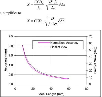
X CCD f D f p z x x y = ⋅ ⋅ ∆ ∆ (6)
which, for a spherical lens, simplifies to
X CCD D f p z x
= ⋅
⋅ ∆ ∆ (7)
The range accuracy of the range sensor is directly related to the separation between the laser plane and the imaging optics (triangulation base), and the focal length of the lens (equation 4). However the field of view of the camera is also related to the focal length of the camera and the CCD dimensions (equation 5). To increase the accuracy of the measurement, for a conventional rotationally symmetric spherical lens, requires to sacrifice the field of view of the sensor (equation 7). Figure 2 shows the relationship between accuracy, field of view, and lens focal length.
4.
ANAMORPHIC LENS
An anamorphic lens gives a different magnification for the two axes -x and -y. The equivalent focal lengths can then be made independent ( fx << fy) and the field of view of the camera larger without sacrificing the range measurement
accuracy (equation 6).
Although distortions are large with anamorphic lens designs, they are not of major concern for range triangulation because of the calibration procedure. Coma and the other primary aberrations may seriously degrade the quality of the optical system and therefore the imaging resolution -x,-y of the device. A tradeoff between cost and optical performance is essential. 0.0 0.5 1.0 1.5 2.0 2.5 0 20 40 60 80 Focal Length (mm) Accuracy (mm) 0 10 20 30 40 50 60 70
Field of View (deg)
Normalized Accuracy Field of View
Figure 2. Range accuracy and Field of View vs. Focal Length of a Lens
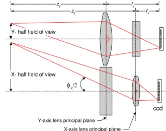
Figure 3 shows the basic principle of an anamorphic lens design, composed of two orthogonal cylindrical lens. Details of the first order geometry are shown in Figure 4. Aberrations of such a simple lens design are very large and in practice other designs using multiple lenses are used. This simple optical system illustrates well the principle behind the anamorphic lens design.
From Figure 4, the magnification ratio of the anamorphic lens system is
M f f a y x = (8)
Of particular importance for calibration is the location of the principal planes of the lens. Obviously, they are very different for the -x and -y axis. The photogrammetric calibration equations (section 5) will not perfectly correct such a large asymmetry in the optical system, although they can easily compensate for a small astigmatism. This is further amplified when the working volume is close to the lens which is usually the case with 3-D triangulation based cameras. In Figure 4, the locations of the primary and secondary planes coincide with the physical location of the lens. For complex lens design, thick lens equations1 are used to compute the location of the primary and secondary principal planes.
5.
LENS DISTORSIONS
The direction of a light ray after refraction at the interface between two homogeneous, isotropic media of differing index of refraction is given by the well known Snell's Law
( )
( )
n1⋅sinθ1 =n2⋅sinθ2 (9)
where both angles are measured from the surface normal. Optical design packages, such as the one used to draw figure 3, trace many optical rays through the system and, applying Snell's Law at each interface, determine the imaging characteristics of a lens or lens system. In practice, the lens system is first estimated by using certain approximation. These basic approximations are based on the sine functions in Snell's Law expanded in infinite Taylor series:
( )
sin ! ! ! θ = −θ θ3 +θ5 −θ7+ 3 5 7 L (10)Figure 3. Basic Anamorphic Lens Design using two orthogonal cylindrical lenses
X- half field of view
ccd
X-axis lens principal plane Y-axis lens principal plane
fx
fy
Y- half field of view
zx
zy
φx/2
The first order and most commonly used approximation replaces sin
( )
θ ≈θ. Although this first approximation called "first order theory" or paraxial theory seems an oversimplification, it is of great utility in determining system focal length, magnification, field of view, and is always used in designing an optical system. In practice the exact optical design of a commercial lens is rarely given by the manufacturer: (lens curvatures, surfaces' distances, glasses) the paraxial theory is often the only one available for a given optical system.The second approximation uses the first two terms in the Taylor expansion of equation 10 (sin
( )
θ ≈ −θ θ3/ !3 ). The results of third order lens aberrations were investigated extensively by Seidel and are therefore often called the Seidel aberrations. Seidel developed a formalism to approximate these aberrations without the necessity of actually tracing large number of rays. The aberrations that are of interest with monochromatic laser based range sensors are:• Spherical aberrations
• Astigmatism
• Coma
• Field curvature
• Distortion
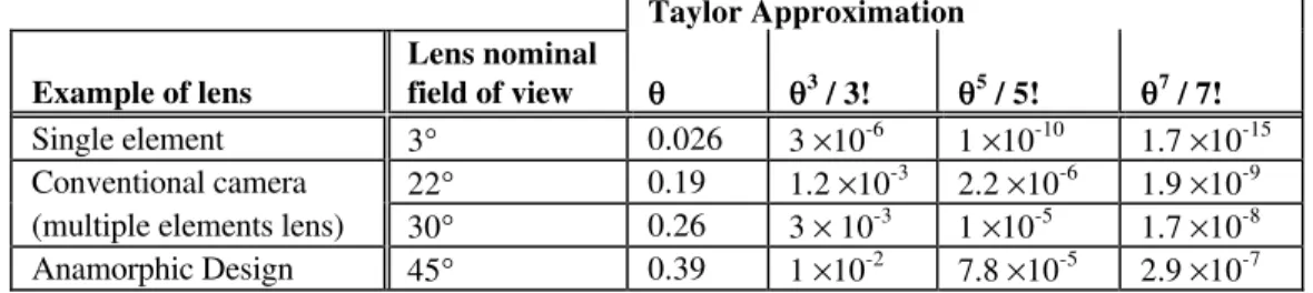
The weight of the different Taylor expansion terms for different field of views are given in Table 1 and shows the possible effect of the different terms when calibrating a lens. Seidel aberrations are usually sufficient to model long focal length and/or small fields of view optical systems.7
For the anamorphic design, the errors associated with the fifth order aberration term will be close to 10-4, more than 30× the error of a 22° field of view lens. Considering that sub-pixel measurement with an accuracy of 1/4 to 1/8 of a pixel gives a sampling resolution of up to 4000 elements on the CCD detector, these aberrations are not negligible for a range sensor. Taylor Approximation Example of lens Lens nominal field of view θθ θθ3 / 3! θθ5 / 5! θθ7 / 7! Single element 3° 0.026 3 ×10⁻⁶ 1 ×10⁻¹⁰ 1.7 ×10⁻¹⁵ Conventional camera 22° 0.19 1.2 ×10⁻³ 2.2 ×10⁻⁶ 1.9 ×10⁻⁹ (multiple elements lens) 30° 0.26 3 × 10⁻³ 1 ×10⁻⁵ 1.7 ×10⁻⁸
Anamorphic Design 45° 0.39 1 ×10⁻² 7.8 ×10⁻⁵ 2.9 ×10⁻⁷
Table 1. Contribution of the Taylor approximation to a lens system aberrations
6.
CALIBRATION MODEL
6.1 Photogrammetry model
Given an homogeneous world coordinate system, Xw, in which 3-D positions are specified, and an homogeneous system, xc, in which pixel locations on the camera CCD are measured, the perspective transformation matrix C can be modeled by a 3×4 matrix:
xc = ⋅C Xw (11)
The calibration method based on a pin-hole optical model of the camera and projector can be simultaneously solved for both intrinsic parameters (e.g., focal length of lens, camera pixel sizes) and extrinsic parameters (e.g., camera orientation).6 However important, lenses optimized for photography have large distortions and principal points offset that must be calibrated. Parameters from these estimates will be included in subsequent data processing for calibration of the raw measurements.
Variations in angular magnification with angle of incidence are interpreted as radial lens distortions, usually expressed as a polynomial function of the radial distance from the optical axis of the lens. Tangential lens distortion is the displacement of a point in the image caused by misalignment of the components of the lens. The displacement is described by two polynomials, one for the displacement in the direction of the -x axis and the other for the displacement in the -y direction:6
[
]
[
]
∂x r K r K r K r xc P r xc P xc yc = ⋅1 1⋅ + ⋅ + ⋅ ⋅ + ⋅ + ⋅2 + ⋅ ⋅ ⋅2 3 2 5 3 7 1 2 2 2 (12)[
]
[
]
∂y r K r K r K r yc P r yc P xc yc = ⋅1 1⋅ + ⋅ + ⋅ ⋅ + ⋅ + ⋅2 + ⋅ ⋅ ⋅2 3 2 5 3 7 2 2 2 1 (13) where r xc yc 2 = 2 + 2 ,xc= −x xo, yc = −y yo. Equation 11 becomesx
c+
∂
c= ⋅
C X
w (14)6.2 Elimination of the z dependency in the model
Using the previous model for calibration does not provide enough parameters to completely model the anamorphic lens. Distortion equations 12 and 13 need other parameters that depend on the zc coordinate of the camera. This is mainly due
to the origin of the principal planes of the lens that are different for the -x and -y axis.
If we specify the rigid transformation from the world coordinate system to the laser plane coordinate system C X⋅ w =Cl⋅Xl, where
X
l=
[
x
l0
z
l]
T then the dependence between world coordinates yw and zw is removedand the intrinsic parameters of the camera can be directly measured. The symmetry of equations 12 and 13 is no longer valid because of the orientation of the laser plane that may not coincide with the CCD/lens optical axis.
We will consider here only equation 1, knowing that the same discussion applies for equation 2. Equation 1 assumes that the position of the center of the CCD and the location of the principal plane of the lens are perfectly known which, in practice, is not the case.
6.3 Anamorphic model
Assuming good quality lens, the calibration equation is
(
)
z
l
l
f
f D l
p
p
z
p o oy=
+
−
⋅ ⋅
⋅
−
+
+
−1
1δ
(15)where zoy and po are the "zero" positions or respectively the lens principal plane and the position of the optical axis of
the lens on the CCD. The zl coordinate in the laser plane is
zp = ⋅zl cos( )τ (16)
where τ is the angle of the laser plane with respect to the z axis of the camera. Assuming that zoy is small, compensated
by the series expansion, then
W i j u p i j j J i I = ⋅ ⋅ = − = −
∑
∑
α, 0 1 0 1 (18)Experimentation and tests using an optical design package have demonstrated that with I=4, J=7, a very good correction of the distortions of the camera-lens (including zoy) is obtained. This is in agreement with Table 2.
Using matrix notation, equation 17 is rewritten in a more convenient form
W=UT⋅Mw P⋅ (19)
where M is a I×J matrix that contains the intrinsic calibration parameters of the sensor and
UT = − 1 2 1 u u K uI ,
PT = − 1 2 1 p p K pJ .And the orthogonal coordinate x, for a first order system is
(
)
xp = zp−zox ⋅tan( )ϑ ϑ = − u u f p o (20)where up is the pixel position (video line) on the CCD, and uo the position of the optical axis of the system, on the CCD.
Note that zoy≠ zox, and xp =xl. Replacing by a Taylor expansion, to calibrate for the distortions, yields
tan( )ϑ =β0+ ⋅β1 +β2⋅ +β ⋅ + 2 3 3 up up up L (21) X =UT⋅Mx Z⋅ (22)
7.
CALIBRATION PROCEDURE
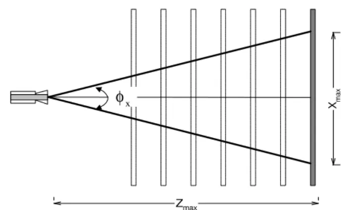
The calibration procedure consists of acquiring several profiles of a calibration bar at perfectly known ranges with increments Zinc.7 Calibration of the Z axis is done with the calibration bar perpendicular to the translation axis of the
camera or the calibration bar as shown in Figures 5 and 6.
From the different sets of measurements zc,p, minimization of the least square error
εi Zc =UT⋅Mw P⋅ − 1 2 (23) Zmax
φ
x XmaxFigure 6. Calibration of the Z axis
Translation stage Rotation stage Calibration bar Zmax x z Sensor φx
directly yields to the calibration matrix Mw of dimensions I × J that will be used to compute range from the raw data (equations 17 and 18). Although in theory it is possible to use some symmetry of the optical design, decentering of the lens and the lack of perpendicularity of the optical planes offset the gain obtained by a non-linear minimization of the calibration equation.
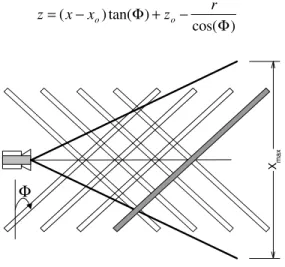
Rotation and translation of the calibration bar are accurately controlled by motorized rotation and translation stages, Figure 5. The equation of the plane of Figure 7 is
z=(x−xo) tan( )+ −zo r cos( )
Φ
Φ (24)
Assuming φ=0, we have the condition zc =zo−r, the Zc range measurements or equation 23. The axis x −∞ < < ∞x ,
is undefined. Let define two plane anglesΦ1= γ , and Φ2= −γ , assuming the referencexo =0 then z1=xtan( )+zo− r cos( ) γ γ (25) z2= x − +zo− r − tan( ) cos( ) γ γ (26) which yield x=1 z −z 2 1 2 ( ) tan( )γ (27)
Calibration of the -x coordinate system can be implemented by independently minimizing the error associated when calibrating for the two angles
zc = ⋅U Mx1⋅Z1 (28)
zc = ⋅U Mx2⋅Z2 (29)
where zc is the position of the calibration plane referenced to the calibration of the z data (equation 22). With
[ ]
ZT = 1 z , calibration of the -x axis is obtained by
x= ⋅U Mx Z⋅ (30)
(
)
Mx= Mx1 Mx2 ⋅ − 1 2 tan( )γ (31) XmaxΦ
8.
EXPERIMENTATION
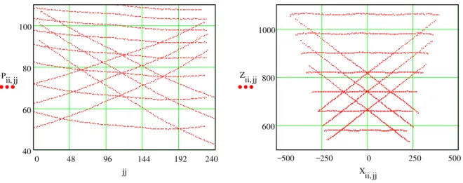
The technique has been applied to different models of standard lens and anamorphic designs. Figure 8 shows the raw data and distortions associated with one of these lenses, using the calibration method discussed in this paper. For this particular lens, we have fx=8 mm, fy=16 mm, and CCD=8.8 mm (2/3” CCD). Distortions are not perfectly symmetric
with the optical axis. Adjustment of the laser plane is referenced to the mechanical body of the camera and not the CCD. That explains the tilted laser profiles of Figure 8.
Figure 9 shows the calibrated X-Z data. Figure 10 shows the RMS error associated with the measurements, obtained with the anamorphic design. Of particular interest is the variation of the field of view of the camera with range which is easily explained by the fact that the reference z=0 of the camera is located at the principal plane of the lens fy while the
field of view is referenced to fx.
The accuracy of the calibrated range data has also been tested using a different method, to validate the accuracy of the measurements.8 This method used targets at perfectly known locations. Absolute accuracy of the measurements was confirmed. Angles between calibration planes can be recovered from the measurements.
500 250 0 250 500 600 800 1000 Z , ii jj X , ii jj
Figure 9. Calibrated range data
0 48 96 144 192 240 40 60 80 100 P , ii jj jj
Figure 8. Raw data
0 0.5 1 1.5 2 2.5 3 580 660 740 820 900 980 1060 1140 1220 Range (mm) RMS Error (mm) 44 45 46 47 48
Field of View (deg)
Accuracy Field of view
10.
CONCLUSION
This paper has presented a method used to calibrate an anamorphic lens for a triangulation based laser range sensor. The principal advantage of using an anamorphic lens for range sensing lies in the independence between the field of view of the camera and the accuracy of the measurement introduced by the anamorphic design. Range accuracy can be increased without sacrificing the field of view of the sensor.
The non-linearity and the distortions of the model of the anamorphic lens were expanded in Taylor series. The linear set of equations was solved to minimize the errors associated with measuring a set of parallel calibration bar at different known ranges. Experimental results have demonstrated that the very strong distortions introduced by the anamorphic lens are easily compensated for with the calibration procedure presented in this paper.
REFERENCES
1. Warren J. Smith, "Modern Optical Engineering, The Design of Optical Systems", 2nd Edition, McGraw-Hill, 1990. 2. Warren J. Smith, "Modern Lens Design, A ressource Manual", McGraw-Hill, 1992.
3. F.Blais, M.Rioux, J.Domey, "Compact Three-Dimensional Camera for Robot and Vehicle Guidance", Optics and Lasers in Engineering, 10 (1989), p. 227-239.
4. Eugene Hecht, Alfred Zajac, "Optics", Addison-Wesley, 1979.
5. F.Blais, M. Lecavalier, J.Domey, P.Boulanger, J.Courteau, "Application of the BIRIS Range Sensor for Wood Volume Measurement", NRC Report ERB-1038, 1992.
6. Atkinson Editor, “Close Range Photogrammetry and Machine Vision”, Chap. 6, Whittles Publishing, Scotland UK, 1996.
7. J.-A. Beraldin, M. Rioux, F.Blais, G.Godin, R.Baribeau, “Calibration of an Auto-synchronized Range Camera with Oblique Planes and Collinearity Equation Fitting”, NRC Report ERB-1041, November 1994.
8. J.-A. Beraldin, S.F. El-Hakim, F. Blais, “Performance Evaluation of Three Active Vision Systems Built at the National Research Council of Canada”, Optical 3-D Measurement Techniques III, Vienna, Oct. 2-4, 1995, p.352-361.