Publisher’s version / Version de l'éditeur:
Journal of Applied Intelligence, 7, 2, 1997
READ THESE TERMS AND CONDITIONS CAREFULLY BEFORE USING THIS WEBSITE.
https://nrc-publications.canada.ca/eng/copyright
Vous avez des questions? Nous pouvons vous aider. Pour communiquer directement avec un auteur, consultez la première page de la revue dans laquelle son article a été publié afin de trouver ses coordonnées. Si vous n’arrivez pas à les repérer, communiquez avec nous à PublicationsArchive-ArchivesPublications@nrc-cnrc.gc.ca.
Questions? Contact the NRC Publications Archive team at
PublicationsArchive-ArchivesPublications@nrc-cnrc.gc.ca. If you wish to email the authors directly, please see the first page of the publication for their contact information.
Archives des publications du CNRC
This publication could be one of several versions: author’s original, accepted manuscript or the publisher’s version. / La version de cette publication peut être l’une des suivantes : la version prépublication de l’auteur, la version acceptée du manuscrit ou la version de l’éditeur.
Access and use of this website and the material on it are subject to the Terms and Conditions set forth at
Comparative Performance of Rule Quality Measures in an Induction System
Dean, P.; Famili, Fazel
https://publications-cnrc.canada.ca/fra/droits
L’accès à ce site Web et l’utilisation de son contenu sont assujettis aux conditions présentées dans le site LISEZ CES CONDITIONS ATTENTIVEMENT AVANT D’UTILISER CE SITE WEB.
NRC Publications Record / Notice d'Archives des publications de CNRC:
https://nrc-publications.canada.ca/eng/view/object/?id=ac437f90-e514-47b5-9105-bbbc8ef15d45 https://publications-cnrc.canada.ca/fra/voir/objet/?id=ac437f90-e514-47b5-9105-bbbc8ef15d45
List of Tables:
Table 1: An example of output
Table 2: Example of Contingency Table
Table 3: Example of Initial Output
List of Figures:
Fig. 1: The Venn Diagram
Fig. 2: Testing and evaluation process
Fig. 3: Graph of Quality Measures versus Problem Definition
Key Words:
- Intelligent Manufacturing - Rule Quality - Machine Learning - Induction - Post-processingContact Author:
A. Famili
Institute for Information Technology National Research Council Canada Ottawa, Ontario, Canada K1A 0R6
famili@ai.iit.nrc.ca Phone: (613) 993-8554
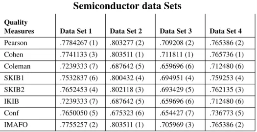
Table 4: Final Evaluation Results
Semiconductor data Sets
Quality
Measures Data Set 1 Data Set 2 Data Set 3 Data Set 4
Pearson .7784267 (1) .803277 (2) .709208 (2) .765386 (2) Cohen .7741133 (3) .803511 (1) .711811 (1) .765736 (1) Coleman .7239333 (7) .687642 (5) .659696 (6) .712480 (6) SKIB1 .7532837 (6) .800432 (4) .694951 (4) .759253 (4) SKIB2 .7652453 (4) .802118 (3) .693429 (5) .762135 (3) IKIB .7239333 (7) .687642 (5) .659696 (6) .712480 (6) Conf .7650050 (5) .675323 (6) .654427 (7) .736773 (5) IMAFO .7755257 (2) .803511 (1) .705969 (3) .765386 (2)
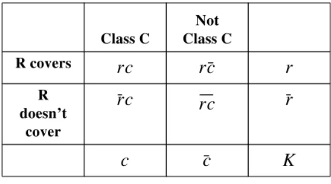
Table 2: Example of Contingency Table
where = the number of examples covered by Rule R that are in Class C. = the number of examples covered by Rule R that are not in Class C. = the number of examples not covered by Rule R that are in Class C.
= the number of examples covered by neither Rule R or Class C. = total number of examples covered by rule R.
= total number of examples not covered rule R. = total number of examples in class C.
= total number of examples not in class C. = total number of examples.
Class C Not Class C R covers R doesn’t cover rc rc r rc rc r c c K rc rc rc rc r
r
c
c
K
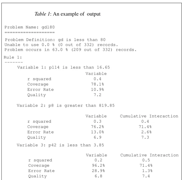
Table 1: An example of output
Problem Name: gdl80 ===================
Problem Definition: gd is less than 80 Unable to use 0.0 % (0 out of 332) records.
Problem occurs in 63.0 % (209 out of 332) records. Rule 1:
Variable 1: p114 is less than 16.65 Variable r squared 0.4 Coverage 78.1% Error Rate 10.9% Quality 7.2 Variable 2: p8 is greater than 819.85
Variable Cumulative Interaction r squared 0.3 0.4
Coverage 76.2% 71.4% Error Rate 13.0% 2.6% Quality 6.9 7.3 Variable 3: p42 is less than 3.85
Variable Cumulative Interaction r squared 0.2 0.5
Coverage 96.2% 71.4% Error Rate 28.9% 1.3% Quality 6.8 7.4
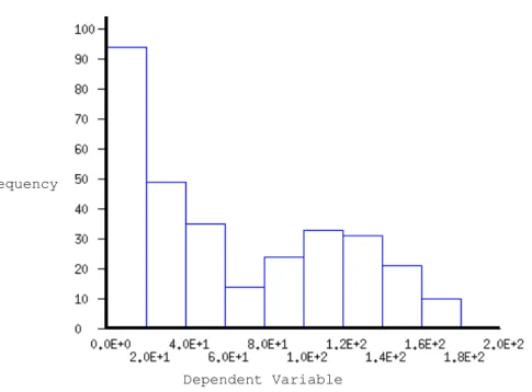
Figure 4: Histogram of Good Dies for Data Set 4
Frequency
Figure 3: Graph of Quality Measures vs. Problem Definition for Data Set 4 0.2 0.3 0.4 0.5 0.6 0.7 0.8 0.9 1 40 50 60 70 80 90 100 110 120 "pearson4" "cohen4" "coleman4" "SKIB14" "SKIB24" "IMAFO4"
Problem Definition Threshold Quality
Measure-ment
Run IMAFO
ten times on
Gather the “best rules”
as selected by each
Quality Measure.
66%
33%
Evaluate the “best rule” cho-sen by each quality measure on the training data. Then assign a value to each
meas-ure based on the accuracy, coverage, false-positive rate
(split by current problem definition)
repeat for next
Fig. 2: Testing and evaluation process
Fig. 1: The Venn Diagram
K T = Target
R = Rule
K = # of records in a data set
Coverage = Error Rate = | T
∩
R | | T | | R — T | | T∩
R | False Negatives False Positives Predicted Actual T R True Positives26. L. Torgo, “Controlled Redundancy in Incremental Rule Learning”, European
Work-shop on Machine Learning. Springer-Verlag. pp.185-195, 1993.
27. L. Torgo, “Rule Combination in Inductive Learning”, European Workshop on
Machine Learning. Springer-Verlag. pp. 384-389, 1993.
28. S.M. Weiss, C.A. Kulikowski, Computer Systems that Learn, Morgan Kaufmann Publishers, San Mateo, CA, 1991.
11. P. Clark and T. Niblett, “The CN2 Induction Algorithm”, Machine Learning
Jour-nal, vol. 3(4), pp.261-283, 1989.
12. A. Famili, and P. Turney, “Intelligently helping human planner in industrial process planning”, AIEDAM, 5(2), 109-124, 1991.
13. A. Famili, “Use of decision-tree induction for process optimization and knowledge refinement of an industrial process, AIEDAM, 5(2), 109-124, 1994,
14. A. Famili, “The Role of Data Pre-processing in Intelligent Data Analysis’’,
Interna-tional Symposium on Intelligent Data Analysis, InternaInterna-tional Institute for Advanced
Studies in Systems Research and Cybernetics, pp. 54-58,1995.
15. O. Gur-Ali and W.A. Wallace, “Induction of Rules Subject to a Quality Constraint: Probabilistic Inductive Learning”, IEEE Transaction on Knowledge and Data
Engi-neering, 5(3), 979-985, 1993.
16. W. Mendenhall, Introduction to Linear Models and the Design and Analysis of
Experiments. Duxbury Press, Belmont, CA, 1968.
17. R.S. Michalski, I. Mozetic, and J. Hong, “The AQ15 inductive learning system: an overview and experiments”, Technical report ISG 86-20, UIUCDCS-R-86-1260, Dept. of Computer Science, University of Illinois, Urbana, 1986.
18. J.R. Quinlan, “Simplifying decision trees”, International Journal of Man-Machine
Studies, 27(3), 221-234, 1987.
19. J.R. Quinlan, “Generating Production Rules from Decision Trees”, Proceedings of
the Tenth International Joint Conference on Artificial Intelligence, Morgan Kaufmann
Los Altos, CA. pp. 304-307,1987.
20. J.R. Quinlan, “Induction of Decision Trees”, Machine Learning, vol. 1, pp.261-283, 1989.
21. J. R. Quinlan, C4.5: Programs for Machine Learning, Morgan Kaufmann Publish-ers. San Mateo, CA, 1993.
22. J. R. Quinlan, “The Minimum Description Length Principle and Categorical Theo-ries”, Proceedings of 11th International Conference on Machine Learning, pp. 233-241, 1994.
23. J. R. Quinlan, “MDL and Categorical Theories (Continued)”, Proceedings of 12th
International Conference on Machine Learning, pp. 464-470, 1995.
24. P. Riddle, R. Segal and O. Etzioni, “Representation Design and Brute-Force Induc-tion in a Boeing Manufacturing Domain, Applied Artificial Intelligence, (8), pp.125-147, 1994.
25. J. Rissanen, “Modeling By Shortest Data Description”, Automatica, vol. 14, pp.465-471, 1978.
Acknowledgements
The authors would like to acknowledge Mike Neudorf, Paul Muysson, and Brian Wen-zel of Mitel Semiconductor for providing us with the data and collaborating on the project. We would also like to thank Peter Turney of the NRC for his useful suggestions on the testing and evaluation process and Prof. Mayor Alvo of Ottawa University for insightful discussions about our research. Evelyn Kidd of NRC gave us valuable com-ments on an earlier version of this paper. IMAFO is licensed to Quadrillion Corp., and is available commercially under the name of Q-Yield.
References
1. T.W. Anderson and S.L. Sclove, The Statistical Analysis of Data, Second Edition. The Scientific Press, Palo Alto, CA, 1986.
2. C. Apte, S. Weiss, and G. Grout, “Predicting Defects in Disk Drive Manufacturing: a Case Study in High-Dimensional Classification”, Proc. of the 9th Conf on AI for
Appli-cations, pp. 212-218, 1993.
3. F. Bergadano, S. Matwin, R. S. Michalski, and J. Zhang, “Measuring Quality of Con-cept Descriptions”, Proceedings of the third European Working Session on Learning, IOS Press, Amsterdam. pp. 1-14, 1988.
4. Y. M. M. Bishop, S.E. Fienberg, and P.W. Holland, Discrete Multivariate Analysis:
Theory and Practice, The MIT Press, Cambridge, MA, 1975.
5. P. B. Brazdil, L. Torgo, Current Trends in Knowledge Acquisition. IOS Press, Amsterdam, 1990.
6. I. Bruha, S. Kockova, “Quality of Decision Rules: Empirical and Statistical Approaches”, Informatica (17) pp. 233-243, 1993.
7. I. Bruha, “Combining Rule Qualities in a Covering Learning Algorithm, Machine Learning workshop, Canadian AI Conference, 1992.
8. J. Canning, “A Minimum Description Length Model for Recognizing Objects with Variable Appearances”, IEEE Transactions on Pattern Analysis and Machine
Intelli-gence, 16(10), pp. 1032-1036, 1994.
8. 9. V.G. Dabija et al, “Learning to Learn Decision Trees”, Proceedings of the
Ameri-can Conference on Artificial Intelligence, AAAI-MIT Press: 88-95, 1992.
10. P. Clark and S. Matwin, “Using Qualitative Models to Guide Inductive Learning”, in Proc. 10th International Machine Learning Conference, Univ. of Mass, USA, pp. 49-56, 1993.
6.0 Conclusions
This research began with the development of the IMAFO induction system. This data analysis tool has been successfully applied in several domains, including semiconduc-tor manufacturing. In spite of these successes, IMAFO’s results could be difficult to interpret. The goal of this project was to overcome this problem by providing IMAFO with a reliable rule quality measure.
This task proved to be a difficult undertaking. First a variety of possible quality meas-ures were identified for examination. Then a methodology was developed for testing and evaluating these measures, and four data sets of semiconductor data selected for examination. The testing process itself was highly automated and required a minimum amount of human interaction. A total of 80 output files were produced, collated, and summarized to produce the final results.
The following are the most important conclusions from our work:
• Some quality measures do indeed perform better than others. Cohen’s statistic was
the over-all best quality measure examined, with several other quality measures receiving very similar results. This is the result of extensive testing and evaluation process that involved applying four performance measures on the rules selected by each quality measure. With this information in hand, it should be possible to develop more effective induction systems and rule post-processing mechanisms for real world domains.
• Some quality measures may be sensitive to the distribution of the data under
exami-nation. While further examination of this area is probably necessary before firm con-clusions can be made, it would appear that some quality measures will indeed reflect the underlying distribution of the data.
Much work remains to be done. In particular, we have examined the use of these quality measures only in post-processing. Their application at some earlier level of the induc-tive process might produce some interesting results. Similarly, further research into the effect of different data set distributions, particularly of the dependent variable, on our quality measures might be worth investigating. One way to examine these effects might be with qualitative models such as those used in Clark and Matwin[11].
The highest rule qualities were reported when the problem was defined as the depend-ent variable < 40. This corresponded with the strong left-tail of the histogram. As the problem definition threshold was increased, the area of the histogram in the target class grew. This caused the values reported by the quality measures to decline, since the most significant feature of the histogram was this tail, and it grew more obscured as more data records were added to the target class. Pearson’s and Cohen’s statistics appeared particularly sensitive to these distribution effects, while Coleman’s statistic was consist-ently unresponsive.
When these final files were examined, some interesting patterns emerged. The quality measure that performed best overall was Cohen’s statistic, with several other measures having nearly equivalent scores. The final results are given in Table 4:
---Approximate Location of Table 4
---A quick glance at these results shows that Pearson’s, Cohen’s, and the IM---AFO statistics were the top three on every data set, while the SKIB1 and SKIB2 measures placed fourth and fifth in most cases. All five of these measures would appear to have some use in practice. However, Coleman’s statistic, the IKIB measure and the Confidence Set sta-tistic placed at the bottom of this list for almost every data set. This poor performance can be traced to the inability of these measures to reflect the effect of false negatives on the quality of a rule. While this was certainly compounded by the built-in bias of the induction system towards false negatives, this serious omission would appear to render them useless in most real world domains.
5.1 Effect of Target Distribution
A factor investigated was how the distribution of the dependent variable affected the performance of the quality measures. An excellent opportunity to examine this situation was afforded by the fact that the same dependent variable was evaluated at five different thresholds for each data set, giving a variety of different target class distributions. A graph of reported values versus the problem definitions for a particular data set is illus-trated in Figure 3. The Confidence set and IKIB measures have been omitted from the graph since their range of possible values is too wide for representation on the same graph as the other measures:
---Approximate Location of Figure 3
---This can be compared with the histogram for the dependent variable in Figure 4:
---Approximate Location of Figure 4
---The score assigned to each measure was a combination of the four performance attributes discussed earlier. This combination, known as the Equally Weighted Average (EWA) was calculated using the following formula:
It was originally planned to provide different weights for positive and negative errors, and so they were incorporated separately instead of a combined error-rate. We decided against this based on consultations with domain experts, and on the knowledge that such a bias is already incorporated into the alogrithm for pruning the decision tree (as mentioned in Section 3.0).
5.0 Results
Once testing was complete, 80 files containing the scores for each measure on each data set for each problem definition remained. An example of one of these files is shown in Table 3:
---Approximate Location of Table 3
---On average, three distinct rules were selected by our quality measures for each prob-lem. Cohen’s statistic, Pearson’s statistic, and the IMAFO statistic chose the same rule in most circumstances, as did Coleman’s statistic and the IKIB statistic. More interest-ingly, the Confidence Set statistics was prone to choose rules quite distinct from those chosen by the measures. While it performed poorly overall, there were several cases where it selected rules which out-performed all the others by a substantial margin. The inference is that this statistic measures substantially different characteristics of the data than the other measures.
The quantity of data to be evaluated was too large for easy comprehension, so some simplification was performed. The results for each data set were shortened by first com-bining the results for the five problems defined for each site and then amalgamating the three distinct sites and combining them with the average site results. This left a single output file containing the rankings for each measure on the entire data set.
EWA Accuracy+Coverage+(1–PositiveErrorRate) +(1–NegartiveErrorRate) 4
conditions for comparing our rule quality measures, though the absence of a right-tailed distribution was regrettable.
4.2 Technical Details
The testing and evaluation process was highly automated. For each data set a group of initialization files had to be created, one for each problem definition. Then a Perl script was invoked on the initialization files, which automatically found and partitioned the data files (maintaining the distribution of the target classes), invoked the analysis soft-ware 10 times on each initialization file, saving the output. Once the runs were com-plete the script scanned the output files and compiled the list of “best rules” as chosen by each quality measure. The script then loaded the testing file and evaluated the per-formance of those rules on the new data. The results were finally printed to a series of text files. The entire process required approximately 3 days of continuous processing on a Sun SPARC 10 workstation. The only phase that required human interaction was set-ting up the initialization files. This automation greatly simplified the entire tesset-ting and evaluation process.
4.3 Evaluation of Quality Measures
Perhaps the greatest problem encountered in this part of the research was the question of how to compare the quality measures. Any procedure that assigned scores to each measure would itself constitute a quality measure and would raise the question of why that measure was not simply used as the quality measure itself. Furthermore, this meas-ure would itself be as questionable as the measmeas-ures under consideration.
Despite this problem we decided to assign a score to each measure. This decision was based on our prior experience in the area, and on consulations with domain experts. While the measure chosen would not do as a quality statistic in its own right because of it’s empirical nature, it does attempt to quantify our experience with what constitutes a good rule in the domain. Our goal was to find a statistical measure that would reflect these same qualities, while avoiding the arbitrariness that would result if we used the empirical measure itself.
(Figure 2). Special care was taken to ensure that the distribution of target samples (as calculated by the current problem definition) was the same in each set. The analysis was then performed 10 times on the training portion of the data, and the single best rule selected by each quality measure was recorded. These rules were then applied to the testing portion of the data and the performance of the one chosen by each quality meas-ure was calculated. The performance of each rule was measmeas-ured with the following attributes, similar to those suggested as formal measures of classifier performance by Kulikowski and Weiss [28]:
• Accuracy: The ratio of correctly classified cases to the total number of cases.
• Coverage: The ratio of correctly classified positives cases to the total number of
pos-itive cases.
• Positive-Error rate: The ratio of positive-errors to the total number of positives. • Negative-Error rate: The ratio of negative-errors to the total number of negatives.
This information was used to assign a score to each quality measure (See Section 4.4). The procedure was then repeated for each data set and problem definition. Figure 2 illustrates the process of testing and evaluation.
---Approximate Location of Figure 2
---Four data sets from semiconductor manufacturing were used for evaluation. This is a domain where complex problems requiring data analysis are regularly encountered, and so an effective induction tool with a reliable rule quality measure would be very useful.
4.1 Semiconductor Data Sets
The four data sets evaluated were gathered over the course of 1993 from a semiconduc-tor manufacturing operation. Each contained approximately 1400 data records record-ing different process variables for three different sites on a srecord-ingle semiconductor wafer. These records were broken down into four different data files, one for each site and one containing averaged values. In each case, there was a single dependent variable, number of good-dies, for which five thresholds were defined and used as problem defi-nitions. The distribution of this variable varied widely between data sets, with Uniform, Left-Tailed, and U-shaped distributions all in evidence. This provided a wide variety of
While this measure is still very heuristic, its results appear to be valuable, especially in cases where target distributions render other measures unreliable. For this reason it is considered here to be a valuable measure that would be of use in interpreting a rule.
3.2.2 Presenting the Contingency Table
The contingency table itself is capable of giving a good intuitive sense of the perform-ance of a rule. Thus, it might be useful to simply present the contents of the contingency table as an extra piece of useful statistical information. This would provide additional information to help the user evaluate the rule. It might also serve to increase the user’s confidence in the quality measure used, since the raw data it was derived from would be available.
Another way to present the contingency table might be in the form of a scatter plot. If the variable chosen by the rule is placed on the X axis and the dependent variable is placed on the Y, then a vertical line for the rule and a horizontal line for the problem definition would divide the plot into four regions mirroring those of the contingency table. This plot makes the intuitive judgement of the rule much easier then looking at the table alone. For this reason such plots might be excellent additions to the output from the induction system.
3.3 Remaining Problems
The largest remaining problem is that of the distribution of the data. All of the quality measures examined assume that we are dealing with a normal population. In many cases this is simply not true and all measures will become increasingly inaccurate as the distribution of the data gets further from the normal. A solution to this problem would require either pre-processing to normalize the data before analysis, or use of other post-analysis techniques to determine the distribution of the data and adapt the measures applied appropriately.
4.0 Testing and Evaluation Methodology
The testing methodology chosen for this study was the standard train-and-test proce-dure. Each data set was partitioned randomly (66/33) into a training set and a testing set
from the normal. It is hoped that certain measures will deal better with this situation than others and this will be a major criteria in choosing the best measure for future use in IMAFO.
Consideration of Small Sample Size.An example of the distribution problems that
has been encountered is the problem of small sample sizes. Cases have existed where the ratio of the target class to the whole population has been as low as 3% of the whole. In these situations, it is questionable if any rule generated by the system could be signif-icant. The effect of this distribution on the contingency table can be predicted. We would expect that and would be very small (after all, there are not very many
pos-sible cases to cover), while and would tend to be large (since there are so many negative examples). One of the characteristics looked for in a quality measure is the ability to handle this situation. The distribution under consideration is obviously not normal and so all of our measures will all suffer. With this in mind, it would appear that those statistics that take into account the better part of the contingency table
( , and ), can be expected to deal relatively well with
the problem. The measures that do not ( , , and
), can be expected to perform poorly.
3.2 Additional Statistical Information
A variety of other information can also be calculated and presented to help interpret the results of the analysis. While such information was not evaluated in the scope of this project, we thought it was important to recognize its existence and consider adding it to the system output as a measure of additional confidence.
3.2.1 Pessimistic Error Rate
The first such information is the pessimistic error rate, used by Quinlan in his C4.5 decision tree algorithm [21]. The standard error rate is simply the ratio of errors to the total number of cases classified. The pessimistic error rate is the upper bound of a confi-dence interval taken around this error rate. The rationale for this is that the performance of any rule on new data will tend to be worse than its apparent error rate on the training set. So the pessimistic error rate tries to estimate the worst expected rule performance.
rc rc
rc rc
QualityColeman QualitySKIB1 QualitySKIB2
QualityPearson QualityCohen QualityIKIB
So this would have to be used as a minimum bound on rule quality. Like Coleman’s sta-tistic, this measure fails to incorporate the completeness of the rule, with the same con-sequences.
3.1.9 Confidence Sets
A final area of statistical theory that may provide a possible quality measure is confi-dence sets. The probability of event p given an example of class C and the firing of rule R is estimated by Consistency(R). So a random variable
has a chi-squared distribution with one degree of freedom. Therefore:
will give a confidence interval ( , ). The lower bound of the interval, , can be
used as a measure of quality. Its value is given by the following quadratic equation[7]:
where
However, this measure again fails to incorporate the completeness of the rule.
3.1.10 Distribution of the Target Samples
An important issue with all of these quality measures is the distribution of the data set under consideration. All the measures under consideration assume the use of a normal distribution and become increasingly inaccurate as the distribution moves further away
Y2 (rc–r⋅p) 2 r p⋅ --- (rc–r⋅ (1–p)) 2 r⋅ (1–p) ---+ = (16) P Y2≤χ12 α, ( ) 1–α = (17) p1 p2 p1 QCONF( )R rc2 S–rc2 rc 2 rc2–S – 2 4 S⋅ +rc2 – 2 S⋅ ---– + = (18) S = r⋅r+χ12( )α (19)
There is a problem with Coleman’s statistic, in that it does not take into account the
completeness of a rule. This means it is unable to measure the effect of false negatives
on the quality of the rule. Due to the bias inherent in the induction system, which favours false negatives over false positives, this may be problematic.
3.1.7 SKIB1 and SKIB2
The following combinations of Coleman’s and Cohen’s statistics have been suggested as measures that combine the best characteristics of both:
and
These are measures of both Agreement and Association. This means that they take into account the entire 2x2 contingency table when returning a rule quality. The implication is that they will deal well with most target distribution problems that would confuse other measures. They appear to be excellent potential quality measures.
3.1.8 Information Gain
Information theory is another area that is closely related to statistics and may be of some help for quality measurements. The following formula attempts to calculate the information gain resulting from a particular rule:
where all logs are base 2. However this only holds if
QSKIB1( )R QColeman( )R 2+QCohen( )R
3
---⋅
= (12)
QSKIB2( )R QColeman( )R 1+Com R( )
2 ---⋅ = (13) QIKIB( )R c K ----log – +logCon R( ) = (14) Con R( ) c K ----≥ (15)
possible that the current rule filtering process (which trims out unimportant rules before the quality measures are calculated) may make the first problem unlikely to occur in practice, but there does not appear to be an easy solution to the second problem. The formula is as follows:
The resulting values will be in the range 0 to 1, with larger values representing greater levels of association.
3.1.5 Cohen’s Statistic
Cohen’s statistic measures the level of association on the main diagonal of the 2x2 con-tingency table. It works by calculating the difference between the actual association and the predicated association along the diagonal (Associationactual - Associationpredicted). The formula is as follows:
This will return a value between -1 and 1, with negative values representing an inverse relationship between the rule and it‘s target class.
3.1.6 Coleman’s Statistic
Coleman’s Statistic is a measure of the “agreement” between the first column and either row of the contingency table. Here the correct relation is between the first column and the first row. Similar to Cohen’s statistic, this measure is calculated by finding the dif-ference between the actual agreement and the predicted agreement. The formula is as follows:
The value returned will again be in the range -1 to 1, with negative values again very unlikely. QPearson( )R (rc rc⋅ –rc⋅rc) 2 c c r r⋅ ⋅ ⋅ ---= (9)
QCohen( )R K Con R⋅ ( ) ⋅Com R( ) –rc K Con R( ) +Com R( ) 2 ---⋅ –rc ---= (10)
QColeman( )R K Con R⋅ ( ) ⋅Com R( ) –rc K Com R⋅ ( ) –rc
This formula was first used by Torgo [26]. The formula was empirically derived. It seems to give good results in practice, but is difficult to interpret, since there is no pre-cise meaning for any particular value.
3.1.3 Consistency and Completeness
Two measures have been suggested by Torgo for calculating rule quality; these are Con-sistency and Completeness [26]. ConCon-sistency is a measure of how specific the rule is to the problem. The higher the consistency the more precisely the rule covers the class under consideration. Consistency is at its maximum when the rule covers all instances of the target class and no instances outside the target class, that is when there are no positive errors.
Completeness is a measure of how much of the problem domain is covered by the rule. The higher the completeness, the more cases are covered by the rule. Completeness is at its maximum when every instance of class c is covered by the rule, that is when there are no negative errors.
It should be noted that both of these equations return a real value in the range of 0 to 1.
3.1.4 Pearson’s Statistic
The Pearson statistic is derived from the simple chi-squared test applied to the con-tingency table. Its result can be used as a measure for rule quality. However, there are several major problems. Firstly, this measure will return a high quality when either
diagonal of the 2x2 contingency table is large, so if and are small, and if and are large, this formula will return a high rule quality, which is obviously incorrect. Secondly, this formula would have problems with cases where the target class distribu-tion is unusual, since the chi-squared test is built to handle a normal distribudistribu-tion. It is
Con R( ) rc r ---= (7) Com R( ) rc c ---= (8) χ2 rc rc rc rc
3.1 Rule Quality Measures
A number of quality measures were considered for this research. Our decision to focus on statistically derived measures eliminated some of the candidates found in the litera-ture. Some other interesting measures, such as Rissanen’s Minimum Description Length principle, were rejected because we felt they were not particularily applicable to the domain. In the end we decided to evaluate statistics similar to those given in [7] as possible statistical quality measures.
3.1.1 The 2 x 2 Contingency Table
The following 2x2 contingency table [6] relates rule R with class C. This table can be used to derive a variety of statistics using variations on the standard chi-squared test for independence. All of the quality measures examined and reported here, including the one currently used by IMAFO, are derived from this table.
---Approximate Location of Table 2
---3.1.2 The IMAFO Quality Statistic
The current IMAFO quality statistic is a real value between 0 and 10, which is calcu-lated by the following formula:
where is the accuracy of rule R, calculated as follows:
and is the estimate of rule coverage and is calculated as follows:
QIMAFO = (ACT R, ⋅EC) ⋅10 (4) ACT R, ACT R, rc+rc K ---= (5) EC EC rc c ---–1 exp = (6)
• the names of the independent variables that influence the process (variables selected for the nodes of the decision tree, i.e.,p114, p8 andp42),
• the particular threshold below or above which the problem may exist,
• the coverage and error rate that represent the reliability of the relationship.
The rule quality is a combined measure that reflects the accuracy and the estimated cov-erage of the rule. The rule quality is explained in Section 3.1.2 and in this paper is referred to as IMAFO quality.
---Approximate location of Table 1
---Figure 1 shows how coverage and error rate are calculated. For a given set of records K (e.g., 332 examples in Table 1), the coverage is the percentage of the problem that the rule covers, i.e., the number of problems that a rule correctly predicts, out of all occur-rences of the problem in each data set. The error rate is the ratio of the number of incor-rect predictions (the rule predicted an error that did not occur) to the number of corincor-rect predictions (the rule predicted an error and it did occur). From the information pre-sented in Table 1, the process engineers decide which rules make sense and what to do with them.
---Approximate location of Figure 1
---There are a number of issues to consider when the data are analyzed using decision tree induction. For example: (i) the coverage and error rate are not always in the ideal range, this justifies the requirement for a rule quality measure; (ii) the distribution of targets in a data set is not always the same. Therefore, we need a quality measure that represents the coverage, error rate and combinations of false positives, false negatives, true posi-tives and true negaposi-tives, and which is also sensitive to various characteristics of the data.
The approach in this work is therefore to identify and test the most appropriate quality measures and evaluate their sensitivity to characteristics of the data set.
The description length of data K for theory R is therefore the sum of the above.
MDL theory is therefore useful in two aspects: (i) to measure the complexity of a theory as the number of bits needed to represent it (coding cost), (ii) to measure how well the theory fits the data. MDL has been applied in a number of applications among which are [8] and Quinlan’s work [22, 23] applied for evaluating categorical theories. Quinlan further proposed a modification to the MDL method so that it can be used for evaluating rules generated by an induction system [21].
Finally, Riddle et al. [24] propose a rule ranking approach as part of processing and analyzing the results of applying induction to a part manufacturing operation. The idea is to use the additional statistical and rule ranking information to easily interpret and apply the results of induction. This quantification of the rules is done through some sta-tistical tests (e.g.
χ
2) to verify that the pattern discovered by the rule is statistically meaningful, given the entire set of data. This approach filters out rules that have a high accuracy but a low level of statistical significance.3.0 Overview of the Approach
The main motivation for this study was to identify a reliable rule quality measure and investigate its performance in real world applications. This rule quality was used to evaluate and filter the rules generated by an induction system (IMAFO) developed at the National Research Council of Canada. The main role of this system [12, 13] is to analyse data from an industrial process and explain why some productions fail. The learning component is a variation of Quinlan’s ID3 algorithm [20]. Its main function is to analyse the data collected from a process and to search for descriptions of unsuccess-ful productions as defined by the user. For its testing and pruning process, IMAFO has a bias towards the errors of commission (positive errors), which are counted as three times worse than the errors of omission (negative errors).
The data analyzed are in the form of numeric or symbolic attribute vectors, representing different aspects of a production environment (e.g. process variables). Table 1 shows an example of a decision tree generated for one problem that has been converted to a set of rules easily understood by process engineers. The information in the rule consists of:
The inadequacy of the entire rule may also be considered at the node level, where the quality of each node is monitored to be above a certain pre-specified threshold of reli-ability. In this case, the cost (or benefit) of an incorrect (or correct) rule is determined by the user. This information is used to set the minimum reliability of an entire rule or individual variables in the rule (that represent the nodes of a tree).
Rissanen [25] proposed the theory of Minimum Description Length (MDL) that can be used to quantify the fit of different models (in our case rules generated by the learning system) by using the length of the description of the data in terms of the model. The MDL theory, is defined as “the total number of binary digits required to rewrite the observed data, when each observation is given by some precision”. When a theory is induced from a data set K to describe the positive class, it partitions K into two sets -one group that satisfies the theory and another group that do not. Each of these groups is further subdivided on the basis of the items’ true class. The four classes would therefore be: (i) true positives, (ii) true negatives, (iii) false positives, and (iv) false negatives. If the theory is known, each observation can be classified by specifying the false positives for the observations satisfying the theory and false negatives among the rest, i.e. two sets of exceptions. Assuming that a set of observations never consists entirely of excep-tions, an encoding scheme to identify k exceptions in n observations gives the value of k which requires:
However, if K contains T positives and N negatives, a theory with fp false positives and
fn false negatives is satisfied by T+fp-fn observations. The exceptions cost of specifying
data K is given as:
Q R( ) 1 (1+g i( )) i= 1 n
∑
⁄ = (1) E n k( , ) logn n k bits log + = (2) E T( +fp–fn,fp) +E N( +fn–fp,fn)bits (3)quality of rules was measured by two properties: consistency and completeness. Consis-tency of the rules is the ratio of the number of correctly covered cases to its number of covered examples, whereas completeness of a rule is the ratio of the number of cor-rectly covered examples to the number of examples of the same class. The approach, although heuristic, resulted from several experiments and observations made with YAILS (also reported in these papers) on real world problems. This method weighs two properties according to the value of consistency, which is a way of introducing some flexibility and coping with different situations, such as rules covering rare cases or very general rules. Bruha and Kockova [6] evaluated various methods and rule quality mea-sures developed by others [3, 5, 26] and viewed quality of a rule as a combination of its correctness, power, predictability, reliability, and likelihood of success. They classified the rule quality control approaches into empirical and statistical and concluded that all methods of calculating rule quality were applicable. However, the heuristics of a learn-ing algorithm and the method of calculatlearn-ing the rule quality of a classification scheme should be selected together, taking the application into account.
Among the statistical measures introduced in [6] are (i) Cohen’s agreement table [4] in which the actual agreement is compared with the observed agreement. This leads to a measure of agreement that can be used as a quality measure. (ii) Using the same table, Coleman [4] defines a slightly different measure of agreement. Both of these measures of agreement are explained in Section 3.1. Weiss and Kulikowski [28] compare learning systems using their true and apparent error rates or quality measures. True error rate of a learning system is defined as the error rate of the learning system if it was tested on the true distribution of cases in the data set. The apparent error rate of a learning system is the error rate on the sample cases that were used to design or build the learning sys-tem.
The issue of inadequacies in representing the knowledge has also been attributed to poor quality of the rules [9]. The authors in this research suggest that there should be a theory to learn good rules that satisfy the expert’s knowledge. The system KAISER uses heuristics knowledge to build a qualitative measure of goodness/badness of a rule. This is done through a set of improprieties and their combinations that are called grav-ity. If the gravity varies between 0 and 1 in each node of the tree (that represent the vari-ables in the rule), then in a rule with n varivari-ables, the quality is defined as:
performance of these measures and recommend the most suitable one(s) for the induc-tive tool that we have developed for intelligent data analysis.
The particular domain that we will focus on in this paper is intelligent process manage-ment. The data for this study come from an advanced industrial process in which proc-ess monitoring and data collection are relatively automated. The application involves analyzing data from semiconductor manufacturing (wafer fabrication), an environment where the volume of collected data is overwhelming. In such industries, the primary goal of data analysis is to identify the most relevant attributes that influence a process from among hundreds of attributes that are normally measured. In these high-dimen-sional process environments [2], an induction system plays an important role in data reduction through identification and ranking of attributes that influence any specific problem. The results of data analysis included some rules that were not reliable due to such reasons as noise in the data or unmeasured attributes.
The format of the paper is as follows: Section 2 includes work related to rule quality and filtering the results of induction. Section 3 provides an overview of the approach, giving a detailed discussions of all the rule quality measures and statistical information that we have investigated. The entire testing and evaluation strategy is explained in Sec-tion 4 and in SecSec-tion 5 results are presented. SecSec-tion 6 gives discussion and conclu-sions.
2.0 Related Work
While the issue of a rule quality measure has been addressed by several researchers in the past, there is no common view or agreement on one or more reliable rule quality measure(s) and its (their) testing and evaluation in real world applications.
The related work can be divided into two somewhat overlapping categories: (i) rule quality and rule filtering, (ii) rule combination and knowledge integration. Both areas require a rule quality measure that can provide a “symbolic filter” for noisy, imprecise, and unreliable knowledge. However, we will primarily focus on the first area as the lat-ter is not entirely related to our work.
1.0 Introduction
Years of research and development work in inductive learning has resulted in introduc-tion of many algorithms that have been tested and performed well in a number of domains from medical to agriculture, finance to manufacturing. Examples of these algorithms include ID3 [20], C4.5 [21], CN2 [11], and the AQ series of algorithms [17]. Researchers and practitioners have also recognized that applying a standard inductive learning tool, such as the ones listed above, is somewhat of a skill [10]. Two problems are quite common: (i) the inability of the learning algorithms to provide reliable rules under all circumstances and (ii) the lack of a reliable measure of quality that users of these tools, such as knowledge engineers or process engineers at a plant, can refer to and easily interpret and apply the results of the data analysis. This has led researchers to investigate the development and use of post-processing techniques to solve these prob-lems. Such techniques would not only help ordinary users of inductive learning tools to easily understand and apply the results of their data analysis, they could also be helpful in developing the knowledge base for an expert system, which could be partially built through induction.
The output of an induction system is usually presented in the form of rules that can be easily understood and applied by users [18, 19]. The induction system that we have developed [12, 13, 14] is an example. This system will be briefly introduced in Section 3.0. To perform any post-processing on the output of this induction system, we first needed a reliable rule quality method and a fairly accurate rule quality threshold that can be used to identify and filter irrelevant rules under various circumstances such as variations in rule coverage, error rate, and the ratio of positive examples to negative examples in the data set. This study was intended to find a reliable measure that would be used for such a threshold.
The literature, discussed briefly in the next section, includes information about a number of rule quality measures. This paper presents an evaluation strategy for these rule quality measures as well as other statistical information appropriate for evaluation of the results from an induction algorithm. The objective here is to demonstrate the per-formance of these quality measures under a number of conditions that are common in the real world and existed in the data used for this study. We will further evaluate the
Comparative Performance of Rule Quality Measures
in an Induction System
Peter Dean* and A. Famili Institute for Information Technology
National Research Council Canada Ottawa, Ontario, Canada K1A 0R6
umdean01@cc.umanitoba.ca and famili@ai.iit.nrc.ca
Abstract
This paper addresses an important problem related to the use of induction systems in analyzing real world data. The problem is the quality and reliability of the rules gener-ated by the systems. We discuss the significance of having a reliable and efficient rule quality measure. Such a measure can provide useful support in interpreting, ranking and applying the rules generated by an induction system. A number of rule quality and sta-tistical measures are selected from the literature and their performance is evaluated on four sets of semiconductor data. The primary goal of this testing and evaluation has been to investigate the performance of these quality measures based on: (i) accuracy, (ii) coverage, (iii) positive error ratio, and (iv) negative error ratio of the rule selected by each measure. Moreover, the sensitivity of these quality measures to different data distributions is examined. In conclusion, we recommend Cohen's statistic as being the best quality measure examined for the domain. Finally, we explain some future work to be done in this area.
(*) Present address: Dept. of Computer Science, University of Manitoba, Winnipeg, MA, R3T 2N2 Canada.
List of Tables:
Table 1: An example of output
Table 2: Example of Contingency Table
Table 3: Example of Initial Output
List of Figures:
Fig. 1: The Venn Diagram
Fig. 2: Testing and evaluation process
Fig. 3: Graph of Quality Measures versus Problem Definition
Key Words:
- Intelligent Manufacturing - Rule Quality - Machine Learning - Induction - Post-processingContact Author:
A. Famili
Institute for Information Technology National Research Council Canada Ottawa, Ontario, Canada K1A 0R6
famili@ai.iit.nrc.ca Phone: (613) 993-8554
Table 4: Final Evaluation Results
Semiconductor data Sets
Quality
Measures Data Set 1 Data Set 2 Data Set 3 Data Set 4
Pearson .7784267 (1) .803277 (2) .709208 (2) .765386 (2) Cohen .7741133 (3) .803511 (1) .711811 (1) .765736 (1) Coleman .7239333 (7) .687642 (5) .659696 (6) .712480 (6) SKIB1 .7532837 (6) .800432 (4) .694951 (4) .759253 (4) SKIB2 .7652453 (4) .802118 (3) .693429 (5) .762135 (3) IKIB .7239333 (7) .687642 (5) .659696 (6) .712480 (6) Conf .7650050 (5) .675323 (6) .654427 (7) .736773 (5) IMAFO .7755257 (2) .803511 (1) .705969 (3) .765386 (2)
Table 2: Example of Contingency Table
where = the number of examples covered by Rule R that are in Class C. = the number of examples covered by Rule R that are not in Class C. = the number of examples not covered by Rule R that are in Class C.
= the number of examples covered by neither Rule R or Class C. = total number of examples covered by rule R.
= total number of examples not covered rule R. = total number of examples in class C.
= total number of examples not in class C. = total number of examples.
Class C Not Class C R covers R doesn’t cover rc rc r rc rc r c c K rc rc rc rc r
r
c
c
K
Table 1: An example of output
Problem Name: gdl80 ===================
Problem Definition: gd is less than 80 Unable to use 0.0 % (0 out of 332) records.
Problem occurs in 63.0 % (209 out of 332) records. Rule 1:
Variable 1: p114 is less than 16.65 Variable r squared 0.4 Coverage 78.1% Error Rate 10.9% Quality 7.2 Variable 2: p8 is greater than 819.85
Variable Cumulative Interaction r squared 0.3 0.4
Coverage 76.2% 71.4% Error Rate 13.0% 2.6% Quality 6.9 7.3 Variable 3: p42 is less than 3.85
Variable Cumulative Interaction r squared 0.2 0.5
Coverage 96.2% 71.4% Error Rate 28.9% 1.3% Quality 6.8 7.4
Figure 4: Histogram of Good Dies for Data Set 4
Frequency
Figure 3: Graph of Quality Measures vs. Problem Definition for Data Set 4 0.2 0.3 0.4 0.5 0.6 0.7 0.8 0.9 1 40 50 60 70 80 90 100 110 120 "pearson4" "cohen4" "coleman4" "SKIB14" "SKIB24" "IMAFO4"
Problem Definition Threshold Quality
Measure-ment
Run IMAFO
ten times on
Gather the “best rules”
as selected by each
Quality Measure.
66%
33%
Evaluate the “best rule” cho-sen by each quality measure on the training data. Then assign a value to each
meas-ure based on the accuracy, coverage, false-positive rate
(split by current problem definition)
repeat for next
Fig. 2: Testing and evaluation process
Fig. 1: The Venn Diagram
K T = Target
R = Rule
K = # of records in a data set
Coverage = Error Rate = | T
∩
R | | T | | R — T | | T∩
R | False Negatives False Positives Predicted Actual T R True Positives26. L. Torgo, “Controlled Redundancy in Incremental Rule Learning”, European
Work-shop on Machine Learning. Springer-Verlag. pp.185-195, 1993.
27. L. Torgo, “Rule Combination in Inductive Learning”, European Workshop on
Machine Learning. Springer-Verlag. pp. 384-389, 1993.
28. S.M. Weiss, C.A. Kulikowski, Computer Systems that Learn, Morgan Kaufmann Publishers, San Mateo, CA, 1991.
11. P. Clark and T. Niblett, “The CN2 Induction Algorithm”, Machine Learning
Jour-nal, vol. 3(4), pp.261-283, 1989.
12. A. Famili, and P. Turney, “Intelligently helping human planner in industrial process planning”, AIEDAM, 5(2), 109-124, 1991.
13. A. Famili, “Use of decision-tree induction for process optimization and knowledge refinement of an industrial process, AIEDAM, 5(2), 109-124, 1994,
14. A. Famili, “The Role of Data Pre-processing in Intelligent Data Analysis’’,
Interna-tional Symposium on Intelligent Data Analysis, InternaInterna-tional Institute for Advanced
Studies in Systems Research and Cybernetics, pp. 54-58,1995.
15. O. Gur-Ali and W.A. Wallace, “Induction of Rules Subject to a Quality Constraint: Probabilistic Inductive Learning”, IEEE Transaction on Knowledge and Data
Engi-neering, 5(3), 979-985, 1993.
16. W. Mendenhall, Introduction to Linear Models and the Design and Analysis of
Experiments. Duxbury Press, Belmont, CA, 1968.
17. R.S. Michalski, I. Mozetic, and J. Hong, “The AQ15 inductive learning system: an overview and experiments”, Technical report ISG 86-20, UIUCDCS-R-86-1260, Dept. of Computer Science, University of Illinois, Urbana, 1986.
18. J.R. Quinlan, “Simplifying decision trees”, International Journal of Man-Machine
Studies, 27(3), 221-234, 1987.
19. J.R. Quinlan, “Generating Production Rules from Decision Trees”, Proceedings of
the Tenth International Joint Conference on Artificial Intelligence, Morgan Kaufmann
Los Altos, CA. pp. 304-307,1987.
20. J.R. Quinlan, “Induction of Decision Trees”, Machine Learning, vol. 1, pp.261-283, 1989.
21. J. R. Quinlan, C4.5: Programs for Machine Learning, Morgan Kaufmann Publish-ers. San Mateo, CA, 1993.
22. J. R. Quinlan, “The Minimum Description Length Principle and Categorical Theo-ries”, Proceedings of 11th International Conference on Machine Learning, pp. 233-241, 1994.
23. J. R. Quinlan, “MDL and Categorical Theories (Continued)”, Proceedings of 12th
International Conference on Machine Learning, pp. 464-470, 1995.
24. P. Riddle, R. Segal and O. Etzioni, “Representation Design and Brute-Force Induc-tion in a Boeing Manufacturing Domain, Applied Artificial Intelligence, (8), pp.125-147, 1994.
25. J. Rissanen, “Modeling By Shortest Data Description”, Automatica, vol. 14, pp.465-471, 1978.
Acknowledgements
The authors would like to acknowledge Mike Neudorf, Paul Muysson, and Brian Wen-zel of Mitel Semiconductor for providing us with the data and collaborating on the project. We would also like to thank Peter Turney of the NRC for his useful suggestions on the testing and evaluation process and Prof. Mayor Alvo of Ottawa University for insightful discussions about our research. Evelyn Kidd of NRC gave us valuable com-ments on an earlier version of this paper. IMAFO is licensed to Quadrillion Corp., and is available commercially under the name of Q-Yield.
References
1. T.W. Anderson and S.L. Sclove, The Statistical Analysis of Data, Second Edition. The Scientific Press, Palo Alto, CA, 1986.
2. C. Apte, S. Weiss, and G. Grout, “Predicting Defects in Disk Drive Manufacturing: a Case Study in High-Dimensional Classification”, Proc. of the 9th Conf on AI for
Appli-cations, pp. 212-218, 1993.
3. F. Bergadano, S. Matwin, R. S. Michalski, and J. Zhang, “Measuring Quality of Con-cept Descriptions”, Proceedings of the third European Working Session on Learning, IOS Press, Amsterdam. pp. 1-14, 1988.
4. Y. M. M. Bishop, S.E. Fienberg, and P.W. Holland, Discrete Multivariate Analysis:
Theory and Practice, The MIT Press, Cambridge, MA, 1975.
5. P. B. Brazdil, L. Torgo, Current Trends in Knowledge Acquisition. IOS Press, Amsterdam, 1990.
6. I. Bruha, S. Kockova, “Quality of Decision Rules: Empirical and Statistical Approaches”, Informatica (17) pp. 233-243, 1993.
7. I. Bruha, “Combining Rule Qualities in a Covering Learning Algorithm, Machine Learning workshop, Canadian AI Conference, 1992.
8. J. Canning, “A Minimum Description Length Model for Recognizing Objects with Variable Appearances”, IEEE Transactions on Pattern Analysis and Machine
Intelli-gence, 16(10), pp. 1032-1036, 1994.
8. 9. V.G. Dabija et al, “Learning to Learn Decision Trees”, Proceedings of the
Ameri-can Conference on Artificial Intelligence, AAAI-MIT Press: 88-95, 1992.
10. P. Clark and S. Matwin, “Using Qualitative Models to Guide Inductive Learning”, in Proc. 10th International Machine Learning Conference, Univ. of Mass, USA, pp. 49-56, 1993.
6.0 Conclusions
This research began with the development of the IMAFO induction system. This data analysis tool has been successfully applied in several domains, including semiconduc-tor manufacturing. In spite of these successes, IMAFO’s results could be difficult to interpret. The goal of this project was to overcome this problem by providing IMAFO with a reliable rule quality measure.
This task proved to be a difficult undertaking. First a variety of possible quality meas-ures were identified for examination. Then a methodology was developed for testing and evaluating these measures, and four data sets of semiconductor data selected for examination. The testing process itself was highly automated and required a minimum amount of human interaction. A total of 80 output files were produced, collated, and summarized to produce the final results.
The following are the most important conclusions from our work:
• Some quality measures do indeed perform better than others. Cohen’s statistic was
the over-all best quality measure examined, with several other quality measures receiving very similar results. This is the result of extensive testing and evaluation process that involved applying four performance measures on the rules selected by each quality measure. With this information in hand, it should be possible to develop more effective induction systems and rule post-processing mechanisms for real world domains.
• Some quality measures may be sensitive to the distribution of the data under
exami-nation. While further examination of this area is probably necessary before firm con-clusions can be made, it would appear that some quality measures will indeed reflect the underlying distribution of the data.
Much work remains to be done. In particular, we have examined the use of these quality measures only in post-processing. Their application at some earlier level of the induc-tive process might produce some interesting results. Similarly, further research into the effect of different data set distributions, particularly of the dependent variable, on our quality measures might be worth investigating. One way to examine these effects might be with qualitative models such as those used in Clark and Matwin[11].
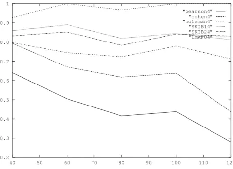
The highest rule qualities were reported when the problem was defined as the depend-ent variable < 40. This corresponded with the strong left-tail of the histogram. As the problem definition threshold was increased, the area of the histogram in the target class grew. This caused the values reported by the quality measures to decline, since the most significant feature of the histogram was this tail, and it grew more obscured as more data records were added to the target class. Pearson’s and Cohen’s statistics appeared particularly sensitive to these distribution effects, while Coleman’s statistic was consist-ently unresponsive.
When these final files were examined, some interesting patterns emerged. The quality measure that performed best overall was Cohen’s statistic, with several other measures having nearly equivalent scores. The final results are given in Table 4:
---Approximate Location of Table 4
---A quick glance at these results shows that Pearson’s, Cohen’s, and the IM---AFO statistics were the top three on every data set, while the SKIB1 and SKIB2 measures placed fourth and fifth in most cases. All five of these measures would appear to have some use in practice. However, Coleman’s statistic, the IKIB measure and the Confidence Set sta-tistic placed at the bottom of this list for almost every data set. This poor performance can be traced to the inability of these measures to reflect the effect of false negatives on the quality of a rule. While this was certainly compounded by the built-in bias of the induction system towards false negatives, this serious omission would appear to render them useless in most real world domains.
5.1 Effect of Target Distribution
A factor investigated was how the distribution of the dependent variable affected the performance of the quality measures. An excellent opportunity to examine this situation was afforded by the fact that the same dependent variable was evaluated at five different thresholds for each data set, giving a variety of different target class distributions. A graph of reported values versus the problem definitions for a particular data set is illus-trated in Figure 3. The Confidence set and IKIB measures have been omitted from the graph since their range of possible values is too wide for representation on the same graph as the other measures:
---Approximate Location of Figure 3
---This can be compared with the histogram for the dependent variable in Figure 4:
---Approximate Location of Figure 4
---The score assigned to each measure was a combination of the four performance attributes discussed earlier. This combination, known as the Equally Weighted Average (EWA) was calculated using the following formula:
It was originally planned to provide different weights for positive and negative errors, and so they were incorporated separately instead of a combined error-rate. We decided against this based on consultations with domain experts, and on the knowledge that such a bias is already incorporated into the alogrithm for pruning the decision tree (as mentioned in Section 3.0).
5.0 Results
Once testing was complete, 80 files containing the scores for each measure on each data set for each problem definition remained. An example of one of these files is shown in Table 3:
---Approximate Location of Table 3
---On average, three distinct rules were selected by our quality measures for each prob-lem. Cohen’s statistic, Pearson’s statistic, and the IMAFO statistic chose the same rule in most circumstances, as did Coleman’s statistic and the IKIB statistic. More interest-ingly, the Confidence Set statistics was prone to choose rules quite distinct from those chosen by the measures. While it performed poorly overall, there were several cases where it selected rules which out-performed all the others by a substantial margin. The inference is that this statistic measures substantially different characteristics of the data than the other measures.
The quantity of data to be evaluated was too large for easy comprehension, so some simplification was performed. The results for each data set were shortened by first com-bining the results for the five problems defined for each site and then amalgamating the three distinct sites and combining them with the average site results. This left a single output file containing the rankings for each measure on the entire data set.
EWA Accuracy+Coverage+(1–PositiveErrorRate) +(1–NegartiveErrorRate) 4
conditions for comparing our rule quality measures, though the absence of a right-tailed distribution was regrettable.
4.2 Technical Details
The testing and evaluation process was highly automated. For each data set a group of initialization files had to be created, one for each problem definition. Then a Perl script was invoked on the initialization files, which automatically found and partitioned the data files (maintaining the distribution of the target classes), invoked the analysis soft-ware 10 times on each initialization file, saving the output. Once the runs were com-plete the script scanned the output files and compiled the list of “best rules” as chosen by each quality measure. The script then loaded the testing file and evaluated the per-formance of those rules on the new data. The results were finally printed to a series of text files. The entire process required approximately 3 days of continuous processing on a Sun SPARC 10 workstation. The only phase that required human interaction was set-ting up the initialization files. This automation greatly simplified the entire tesset-ting and evaluation process.
4.3 Evaluation of Quality Measures
Perhaps the greatest problem encountered in this part of the research was the question of how to compare the quality measures. Any procedure that assigned scores to each measure would itself constitute a quality measure and would raise the question of why that measure was not simply used as the quality measure itself. Furthermore, this meas-ure would itself be as questionable as the measmeas-ures under consideration.
Despite this problem we decided to assign a score to each measure. This decision was based on our prior experience in the area, and on consulations with domain experts. While the measure chosen would not do as a quality statistic in its own right because of it’s empirical nature, it does attempt to quantify our experience with what constitutes a good rule in the domain. Our goal was to find a statistical measure that would reflect these same qualities, while avoiding the arbitrariness that would result if we used the empirical measure itself.