Publisher’s version / Version de l'éditeur:
Vous avez des questions? Nous pouvons vous aider. Pour communiquer directement avec un auteur, consultez la première page de la revue dans laquelle son article a été publié afin de trouver ses coordonnées. Si vous n’arrivez pas à les repérer, communiquez avec nous à [email protected].
Questions? Contact the NRC Publications Archive team at
[email protected]. If you wish to email the authors directly, please see the first page of the publication for their contact information.
https://publications-cnrc.canada.ca/fra/droits
L’accès à ce site Web et l’utilisation de son contenu sont assujettis aux conditions présentées dans le site LISEZ CES CONDITIONS ATTENTIVEMENT AVANT D’UTILISER CE SITE WEB.
2018 IEEE 14th International Conference on Automation Science and Engineering
(CASE), pp. 1400-1405, 2018-12-06
READ THESE TERMS AND CONDITIONS CAREFULLY BEFORE USING THIS WEBSITE. https://nrc-publications.canada.ca/eng/copyright
NRC Publications Archive Record / Notice des Archives des publications du CNRC :
https://nrc-publications.canada.ca/eng/view/object/?id=4a2c0581-f009-4692-a91c-c6c91a1f71d9 https://publications-cnrc.canada.ca/fra/voir/objet/?id=4a2c0581-f009-4692-a91c-c6c91a1f71d9 This publication could be one of several versions: author’s original, accepted manuscript or the publisher’s version. / La version de cette publication peut être l’une des suivantes : la version prépublication de l’auteur, la version acceptée du manuscrit ou la version de l’éditeur.
For the publisher’s version, please access the DOI link below./ Pour consulter la version de l’éditeur, utilisez le lien DOI ci-dessous.
https://doi.org/10.1109/COASE.2018.8560433
Access and use of this website and the material on it are subject to the Terms and Conditions set forth at
Energy performance based anomaly detection in non-residential
buildings using symbolic aggregate approximation
2
Abstract— Building system faults in commercial and office buildings can result in a reduced occupant comfort and increased utility bills. Energy performance-based anomaly detection helps operators efficiently identify faults. In this work, a data-driven method for anomaly detection is presented. Using a symbolic aggregate method, the weekly energy demand profiles are statistically quantised and labeled to determine normal and abnormal building behaviours. A case study with three federal office buildings has been conducted to demonstrate the proposed method. The resulting technology provides building operators with easily-interpreted and actionable information for optimised building performance.
I. INTRODUCTION
Buildings are responsible for about % of end-use energy consumption in developed countries [1]. This implies that increasing energy efficiency of buildings and improving how they are operated can greatly contribute to reduction of both energy costs and greenhouse gas emissions. Although such efforts are usually addressed during the design phase, many studies show that buildings do not perform as expected, and that a majority of energy loss comes from errors occurring either in the construction phase or during the actual lifespan of the building, introduced by deteriorating materials, malfunctioning devices, and non-optimal operating commands [2], [3].
Traditionally, stakeholders tackle the problem of anomalous building systems behaviour by engaging technical consultants to inspect the building and to review energy consumption data. In reality, many non-residential building portfolios such as university campuses, military bases, banks, post offices, etc. are maintained by a limited number of facility operators, who do not have the resources to detect every system malfunction, such as equipment failures and unnecessary lighting during unoccupied periods [4]. Furthermore, with the rise of fully automated buildings, these systems are becoming more sophisticated; a modern non-residential building is often equipped with thousands of energy-related sensors, actuators, and controllers [5]. The resulting streams of raw data from these sensors are typically collected and temporarily stored by the building automation system (BAS) at regular time intervals. Ideally, a building energy management system (BEMS) is placed on top of the BAS, and will archive such data for long-term analysis purposes. At a first glance, this seems to be a great
* The research was supported by the Smart Building Project (A1-006050) of Public Services and Procurement Canada (PSPC) and National Research Council Canada (NRC).
A. Ashouri, Y. Hu, G. Newsham, and W. Shen are with the National Research Council Canada, Ottawa, ON K1A 0R6 CANADA (A. Ashouri is the corresponding author: phone: +1-613-998-6807; fax: +1-613- 954-3733; e-mail: [email protected]).
opportunity for building operators and energy data scientists, given the availability of data-driven tools for building monitoring, benchmarking, and control. However, these systems accumulate a vast amount of data over time, creating new challenges in efficient data interpretation. As a result, building energy researchers have been paying closer attention to methods that can enable them to analyse large building datasets for the purpose of remote auditing and automated anomaly detection. A recent review [6] indicates that researchers are widely targeting the topic of anomaly detection using analyses of the whole building energy demand. The two major approaches used in such analyses are data-driven methods [7] and model-based methods [8]. While model-based approaches are capable of simulating the behaviour of buildings under various boundary conditions, they rely on a relatively detailed level of knowledge about the building structure, parameters, and occupant behaviour. On the contrary, data-driven methods can be deployed more quickly by data analysts, though some knowledge of building physics and systems is essential for meaningful interpretation. In addition, the recent advancements in machine learning and data mining techniques have led to several methods that may be leveraged by building energy scientists [9].
Among the various techniques of data-driven anomaly detection, a method called Symbolic Aggregate approXimation (SAX), first introduced by Lin et al. in 2003 [10], shows superior performance with regards to larger datasets. The SAX method incorporates a value quantisation for given intervals within a data time series, and facilitates large-scale evaluations by reducing the dimension of data from (length of time series) to � (number of “letters” in the SAX “word”) where � << . As a result, many applications of SAX method can be found in the literature for motif selection and anomaly detection [11], [12]. Given these advantages, in this study SAX has been selected as the method to identify anomalous energy behaviour in a group of non-residential buildings.
The rest of the paper is organized as follows. Section II discusses the proposed method and demonstrates the adjustments that distinguished our method from similar works, while Section III is dedicated to the analysis of results for the studied cases and discusses the capabilities of the labeling system for various applications. Three federal government office buildings, referred to as buildings B1, B2, and B3 are investigated in the case study.
Although the proposed method is applicable to various forms of energy demand, our focus in this study is solely on electricity. Furthermore, demand data from building B2 are used to elaborate the deployment of techniques in Section II.
Energy Performance Based Anomaly Detection in Non-Residential
Buildings Using Symbolic Aggregate Approximation*
The anomaly detection method used in this article consists of several modules that were progressively developed and fine-tuned. The modules are responsible for data cleaning, processing, and post-processing analysis. Figure 1 shows a block diagram describing the modules and the connections among them.
The four main modules of the proposed method are
1) Data cleaning: the block where pre-processing of
raw data takes place;
2) Statistical quantisation: the block where demand profiles are transformed into “words”; in this case words are a string of letters than concisely summarize the weekly energy load shape of a building;
3) Motif selection: the block responsible for finding the “Normal”wordandthecorrespondingnormalannual demand; and
4) Anomaly detection: the final block where a
comparison of normal and actual demands is performed, followed by a qualitative labeling of results.
In the followings, each aforementioned block is described in more details.
A. Data cleaning
The anomaly detection process relies on a historical dataset of demand profiles (also referred to as load profile, energy consumption, etc.) corresponding to a single or a combination of collection points in one or several buildings. In the case of data collection for electricity usage, a meter is installed either at the transformer level or right after entering the building. In modern commercial and office buildings, the sensory data are collected and integrated in the BAS which can be access directly, or through a high-level platform such as the BEMS. The latter provides a user-friendly environment to enable building operators to access energy information.
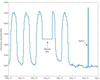
The federal buildings studied in this project are monitored using a BEMS called Kaizen, a commercial product from CopperTree Analytics [13]. Figure 2 shows a sample log of the hourly electricity demand profile for building B2. A brief visual inspection of the data reveals a gap in the first week of the demand profile, plotted as a horizontal line in the figure.
The purpose of the data cleaning module is to handle such gaps in the data, preventing the anomaly detection tool from flagging the period as abnormal while it could simply correspond to a temporary power outage in the sensor or an out-of-memory buffer.
The module involves two main tasks of Outlier Elimination and Missing-Value Imputation. A detailed description of the algorithms used for these tasks is out of the scope of this article and will be discussed elsewhere.
B. Statistical Quantisation
Once the demand profiles are pre-processed and cleaned, the next step is to convert them into a form suitable for anomaly detection. The demand profiles are time series with an hourly resolution. The anomaly detection method incorporates a statistical quantisation technique based on the SAX method to transform profiles into words. The choice of the SAX method for anomaly detection in commercial buildings was inspired by the work described in [14]. However, we propose a more sophisticated approach at the quantisation stage to improve the performance.
Our implementation of the statistical quantisation consists of the following main stages: normalization, temporal division, sampling, and SAX transformation. Each stage is briefly explained in the following sections.
Normalization: This stage involves calculating a standard
score (or z-score) normalized version of the cleaned electricity demand profile �e ec, using
�e ecr a = �⁄ ⋅ �e ec− � (1) where, � is the standard deviation and � is the mean of the electricity demand.
Temporal division: After normalization, a temporal
division of the data according to primary (weekly) and secondary (half-daily) periods is performed. The available dataset has a resolution of 1 hour; hence a weekly profile is presented as a vector with elements. A week, in our definition, starts on a Monday at 6am and ends on the following Monday at 5:59am. The half-daily sections are defined as am − : pm (day time) and pm − : am (night time).
Sampling: In order to reduce the dimension of data, the
weekly demand profiles with hours are averaged for each half-day section, resulting in a vector with a length of .
Figure 1. Block diagram showing the main four modules (in color) and their connections. Data Cleaning Statistical Quantization Motif Selection Anomaly Detection Diagnosis BAS BEMS Normal demand Words O p erato rs Cleaned demand Raw demand Sensor data Rules
As an example, a weekly demand profile for building B2 is shown in Figure 3 with the 12-hour sections and the corresponding averaged demands.
SAX transformation: At the final stage, the SAX method
is applied to the sampled data. As described in [14], SAX is performed by quantising the values in data and transforming them into letters. This means that the demand vector of length that represents a weekly profile will be transformed into a word with letters. The mapping of average values into letters is done by a statistical approach that involves cutting the probability density of the average demands (i.e. the orange lines in Figure 3) into disjoint sets.
The method used for the cutting in most studies (such as [14]) is an equiprobable cut, implying that the probability of occurrence for letters are equal. However, we use a more meaningful approach to select the cut-off thresholds. First we divide the demand set into two groups: The expected-high demands, comprised of the averaged demand values for the day time during weekdays (five values per week), and the expected-low demands, comprised of the averaged demand values during weekends and night time during weekdays (nine values per week). Furthermore, public holidays are treated the same as weekends. These two demand sets are not disjoint but are usually separated well enough so that they can be used to define the cut-off thresholds.
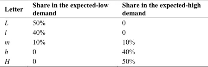
Figure 4 shows the normalized probability density of the average electricity demand for building B2 with the expected high and low demand densities. The cut-off thresholds used for SAX quantisation are calculated as shown in Table 1. The letters (for extreme low demand) and (for low demand) are assigned to a % and % portion of the expected low demand density, respectively. Similarly, the letters � and ℎ are taken from the expected-high demand density, representing extreme high demand and high demand, respectively.
Table 1. The cut-off thresholds used for SAX quantisation.
Letter Share in the expected-low demand
Share in the expected-high demand L 50% 0 l 40% 0 m 10% 10% h 0 40% H 0 50%
The letter , for medium demand, corresponds to the lowest % percent of the expected-high demand and the highest % of the expected-low demand. It is possible that the expected high and low demand densities are not properly separated; hence the number of generated letters might be fewer than five. In such cases, the words will be created using fewer letters, but it does not affect the reliability of the method. For the buildings studied in this article, the expected high and low demands were properly separated.
C. Motif Selection
Once the demand values are mapped into letters, each weekly demand profile is transformed to a 14-letter word. The next step in the statistical anomaly detection method is the selection of a motif in the SAX transformed demand profiles, referred to as a normal word. This is done by counting the frequency of a weekly word appearing within the total observed period, in this case being February 2011 to June 2016.
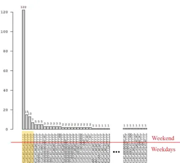
Figure 5 depicts the word frequency for the electricity demand of building B2 (for this visualization, both h and H are shown as H, and both l and L are shown as L). There are 78 distinguished words and, as expected, the word � � � � � has the highest frequency of 122. This word corresponds to a high demand (�) during the weekday mornings and a low demand (L) during weekday evenings as well as the whole weekends. The second most frequent word
is � � � � and the third one is
� � � � with the only difference being the first letter. These two words correspond to weeks when a holiday has fallen on a Monday; hence a lower demand is expected during the working hours. Finally, the fourth most frequent word of � � � � represents weeks when Friday is a holiday and has a lowered demand as a result. These four most frequent words (as highlighted in Figure 5) comprise almost 60% of the weeks. Regardless, only the most frequent word, being � � � � � , is selected as the normal wordorthe“motif”.
Note that the word frequency changes if different cut-off thresholds to those shown in Table 1 are selected. Therefore, in order to assure a robust selection of the normal word, one may perform a sensitivity analysis based on the cut-off values.
Figure 3. Averaged 12-hour sections for building B2. Figure 4. The density for the actual, the expected high, and the expected-low demands, shown for building B2, as well as the resulting cut-off
This procedure is out of the scope of this article and will be discussed elsewhere.
Following the selection of a normal profile, the corresponding normal electricity demand needs to be calculated. In order to decide whether the normal demand is defined over the whole dataset or rather individually for each year, a data screening is performed. Figure 6 shows a compilation of demands on normal word weeks for the six studied years. It is observed that a downward trend in electricity demand exists in building B2, suggesting progressive improvements in the operation and efficiency of electrical devices, such as fans, lighting and plug loads. Similar trends can be observed for the electricity demand in the other two buildings. Therefore, an annual normal demand was calculated for each studied year, from the normal word weeks in each year.
D. Anomaly Detection
Once the annual normal demands are calculated, the actual weekly demands are compared to the normal demand of the corresponding building and anomalies are detected by quantifying the divergence.
Obviously, an energy demand which is lower than expected is translated to a higher grade in performance. This implies that, if a letter H is assigned to a period in the normal profile, there is no need to evaluate that period in the actual profile as a poor performance anomaly, because any existent energy demand is better than or at least equal to a high (i.e. H) demand. Given this knowledge, the three labels are defined as follows:
Good: A Good label is assigned to a week that has a SAX
word matching the pattern _ _ _ _ _ where the underscores can be replaced by any of the five letters (L, l, m, h, H). The Good pattern corresponds to a week when all expected-low periods do indeed have a low demand. Once the Good label is assigned to a week, no weekly saving (�w) is calculated. Note that at this stage the algorithm is not case sensitive, therefore both h and H are treated as H, and both l and L are treated as L. In application, we do not wish to overly distract operators, and therefore choose not to alert operators to relatively small deviations from the ideal normal demand profile.
OK and Bad: If the SAX word of the week does not
follow the Good pattern of _ _ _ _ _ , the weekly demand is compared to the normal demand in order to calculate the potential weekly energy saving using the formula �w=∑ (��,� elec−� �,� elec) � ∑ �� �,�elec × , � ∈ { , , , , , , , , } (2)
where, � indicates the percentage of potential saving, � is the normal demand and � is the actual weekly demand. Index � enumerates the 12-hour sections, and in this case iterates only for the letters that correspond to a low demand periods in the Good pattern. Index � indicates the weeks. Because of the way values of � are selected, the numerator of the fraction is always smaller that the denominator; hence �� is properly defined as a percentage between and . Note that the algorithm treats the holidays and weekend days the same.
The labeling process is based on the value of �w. If it exceeds %, the weekly performance is directly labeled as Bad. Otherwise, it is labeled as OK. The % threshold is a tunable parameter and should be adjusted according to the type of building and the deviation level tolerated by building operators. In the next section, a case study is carried out for the three office buildings in order to demonstrate the potential of the proposed labeling method.
III. CASE STUDY AND DISCUSSIONS
A. Buildings
The case study is based on the archived energy consumption data collected from three federal office buildings located in the city of Ottawa, Canada. Table 2 shows an overview of the buildings’ information.
The selected buildings demonstrate diversity in terms of floor area and the electricity demand which enables a more reliable evaluation of the method.
Figure 5. The word frequency for building B2. Several words in the middle of the chart are ommited. The four most frequent words are highlighted.
Figure 6. Demand profile for all normal weeks for building B2. A downward trend in demand is visible.
Table 2. Parameters of the studied buildings. Building Number of floors Floor area (m2) Construction year Average electricity demand (MWh/yr) B1 1 2,000 1956 195 B2 13 61,000 1979 7,500 B3 2 4,400 1955 360
However, the diversity should not prevent a meaningful comparison of the results among the buildings, which reveals the importance of the normalization stage.
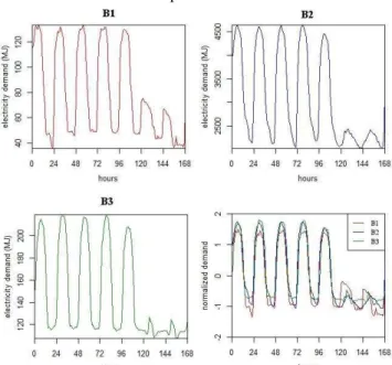
Figure 7 shows the normal demand profiles of the three studied buildings for the year 2015. As expected, the profiles are not alike in shape and magnitude, as they are bound to the characteristics of the buildings and the behaviour of the occupants. Therefore, z-score normalized versions of the profiles are also shown. The normal demands follow a very similar weekly pattern, suggesting similarity in working hours and the behavioural habits of the occupants.
Once the labeled weekly demand profiles are generated for each building and each studied year, the results can be investigated from two different angles: with a focus on label statistics (useful for fault detection and diagnosis (FDD)) and on demand reduction (useful for energy auditing purposes). Both aspects are explored in the following sections.
B. Labeling
Table 3 shows a summary of generated labels for the three buildings and each year of operation based on the SAX method. From an FDD perspective, the main concerns are the anomalies that are non-temporary and severe, hence a higher probability to identify at a systematic fault in the system. This implies that a persistent high number of OK or Bad weeks in any year would raise a red flag.
By reviewing Table 3c, one observes that the first criterion is satisfied by building B3, as a consistently large number of OK weeks can be found, especially in years 2012 to 2015 where a more complete dataset is available.
Using such information, a technician may be able to efficiently allocate their time towards fixing faulty equipment or aberrant operational parameters.
For the second criterion, that is the existence of less frequent but more sever anomalies, building B1 demonstrates an example. In years 2014 and 2015 about % of the weeks are labeled as Bad, pointing to the possibility of a severe fault, which might be behavioural, mechanical, or structural nature. Similarly, the Bad labels of building B2 for the year 2012 add up to %, pointing at a situation that requires further investigation by building operators. One can proceed with a seasonal, daily, or hourly examination of the labels to identify the potential sources of the faults.
C. Potential energy saving
The weekly labels can be used to estimate annual energy savings potential by comparing the actual scenario to one where all weeks are labeled as Good. This is valorized using the annual potential energy saving, calculated as
�a ua =∑ ∑ (��,� elec−� �,� elec) � � ∑ ∑ ��,�elec � � × , � ∈ { , … , W} (3) where, � iterates over the weeks with complete data availability with a maximum of � and � is defined in the same way as Equation (2). Note that the �a ua is also equivalent to the average of �wee y values.
Table 3. Results of anomaly detection for the three studied buildings. Only weeks with enough number of available data points are considered.
Year
(a) Labeled weeks for building B1
Weeks Good OK Bad 2011 32 71% 12 27% 1 2% 45 2012 36 71% 12 24% 3 6% 51 2013 26 58% 16 36% 3 7% 45 2014 26 52% 14 28% 10 20% 50 2015 29 58% 12 24% 9 18% 50 2016 17 71% 7 29% 0 0% 24 Total 166 63% 73 28% 26 10% 265 Year
(b) Labeled weeks for building B2
Weeks Good OK Bad 2011 35 78% 6 13% 4 9% 45 2012 35 69% 8 16% 8 16% 51 2013 31 69% 10 22% 4 9% 45 2014 38 76% 7 14% 5 10% 50 2015 22 44% 27 54% 1 2% 50 2016 15 63% 7 29% 2 8% 24 Total 176 66% 65 25% 24 9% 265 Year
(c) Labeled weeks for building B3
Weeks Good OK Bad 2011 21 47% 24 53% 0 0% 45 2012 16 31% 33 65% 2 4% 51 2013 28 56% 18 36% 4 8% 50 2014 27 54% 23 46% 0 0% 50 2015 30 60% 20 40% 0 0% 50 2016 17 71% 6 25% 1 4% 24 Total 139 51% 124 46% 7 3% 270
Figure 7. Normal weeks in 2015 for the three buildings. The last plot shows a combined overview of normalized profiles which reveals the similarities.
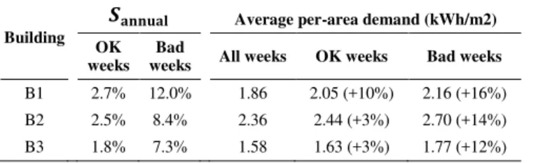
normalized measure for the energy intensity of buildings. The first observation is that the per-area demand values are in the same range for the three buildings, although the absolute electricity demand is much higher for B2 as shown in Table 2.
The second and the more interesting observation is that the saving potential for the OK weeks and the more critical Bad weeks is not proportional to the magnitude of the average per-area demand. For example, by comparing the average demand of Bad weeks between buildings B1 and B3, and energy auditor may conclude that they suffer from the same magnitude of severity in abnormal behaviour, as they demonstrate an increase of 16% and 12% in average weekly demand, respectively. However, the saving potential calculated using the anomaly detection method (Table 3) reveals that in fact, Bad weeks in building B1 are much frequent and require a more urgent investigation. Similar inappropriate wrong conclusions may be made for the OK weeks of buildings B2 and B3.
Table 4. Annual saving and demand per area for the three buildings.
Building
������� Average per-area demand (kWh/m2) OK
weeks Bad
weeks All weeks OK weeks Bad weeks B1 2.7% 12.0% 1.86 2.05 (+10%) 2.16 (+16%) B2 2.5% 8.4% 2.36 2.44 (+3%) 2.70 (+14%) B3 1.8% 7.3% 1.58 1.63 (+3%) 1.77 (+12%)
On the contrary, a comparison of average per-area demand for OK weeks in buildings B1 and B2 may bring the investigator to the conclusion that there is a much bigger saving potential in building B1, while the value of �a ua for OK weeks indicates that it might not be the case.
IV. CONCLUSIONS
The data-driven anomaly detection methods are superior to the model-based methods in the sense that they do not rely on a detailed knowledge of the building structure and parameters in advance. In this work, a statistical data-driven approach using the SAX method was proposed to analyse years of collected data from three federal buildings with diversity in size and electricity demand profiles. In summary, the results of the proposed anomaly detection method reveals that the implemented SAX-based labeling approach can serve as a multi-purpose energy monitoring tool for both operators and stake holders, by transforming the large sets of time series data into the more comprehendible weekly words. As the method relies on normalization and statistical interpretation, a comparison of resulting saving potential among the buildings is facilitated and the conclusions are more meaningful since they are not bound to the specific building properties.
Regarding the potential applications for the proposed approach, we expect that it can be widely applied to large centralized or distributed campuses where a limited number of facility operators are in charge of a large number of buildings (such as universities/colleges, military bases, schools, hospitals, bank branches, postal outlets, etc.). The
electricity demand, the main requirement for the deployment of the method is a reliable demand measurement at a reasonable resolution (finer than or equal to 1 hour). Such data collection is already available at many of the aforementioned locations.
For the future extension of this work, the authors intend to further develop the method and deploy it for anomaly detection in heating and cooling demand profiles. Furthermore, a deployment of the developed algorithm for “realtime”anomalydetectioninnon-residential buildings is planned.
REFERENCES
[1] A.M.Omer,“Energy,environmentandsustainable
development,”Renew. Sustain. energy Rev., vol. 12, no. 9, pp. 2265–2300, 2008.
[2] X.Pang,M.Wetter,P.Bhattacharya,andP.Haves,“A framework for simulation-based real-time whole building performanceassessment,”Build. Environ., vol. 54, pp. 100–108, 2012.
[3] P.DeWilde,“Thegapbetweenpredicted and measured energy performanceofbuildings:Aframeworkforinvestigation,”
Autom. Constr., vol. 41, pp. 40–49, 2014.
[4] J.O’Donnell,M.Keane,E.Morrissey,andV.Bazjanac, “Scenariomodelling:Aholisticenvironmentalandenergy management methodforbuildingoperationoptimisation,”Energy
Build., vol. 62, pp. 146–157, 2013.
[5] B.GunayandW.Shen,“ConnectedandDistributedSensingin Buildings:ImprovingOperationandMaintenance,”IEEE Syst.
Man, Cybern. Mag., vol. 3, no. 4, pp. 27–34, 2017.
[6] C.Miller,Z.Nagy,andA.Schlueter,“Areviewofunsupervised statistical learning and visual analytics techniques applied to performance analysis of non-residentialbuildings,”Renew.
Sustain. Energy Rev., vol. 81, pp. 1365–1377, 2018.
[7] J. E. Seem,“Usingintelligentdataanalysistodetectabnormal energyconsumptioninbuildings,”Energy Build., vol. 39, no. 1, pp. 52–58, 2007.
[8] Z.O’Neill,X.Pang,M.Shashanka,P.Haves,andT.Bailey, “Model-based real-time whole building energy performance monitoringanddiagnostics,”J. Build. Perform. Simul., vol. 7, no. 2, pp. 83–99, 2014.
[9] S.Yin,S.X.Ding,X.Xie,andH.Luo,“Areviewonbasicdata-drivenapproachesforindustrialprocessmonitoring,”IEEE
Trans. Ind. Electron., vol. 61, no. 11, pp. 6418–6428, 2014.
[10] J.Lin,E.Keogh,S.Lonardi,andB.Chiu,“Asymbolic representation of time series, with implications for streaming algorithms,”Proc. 8th ACM SIGMOD Work. Res. issues data
Min. Knowl. Discov. - DMKD ’03, p. 2, 2003.
[11] B.Chiu,E.Keogh,andS.Lonardi,“Probabilisticdiscoveryof timeseriesmotifs,”inProceedings of the ninth ACM SIGKDD
international conference on Knowledge discovery and data
mining, 2003, pp. 493–498.
[12] J.Lin,E.Keogh,L.Wei,andS.Lonardi,“Experiencing SAX: a novelsymbolicrepresentationoftimeseries,”Data Min. Knowl.
Discov., vol. 15, no. 2, pp. 107–144, 2007.
[13] CopperTree,“Kaizen-building-energy.”[Online].Available: http://www.coppertreeanalytics.com/kaizen-building-energy/. [14] C.Miller,Z.Nagy,andA.Schlueter,“Automateddailypattern
filteringofmeasuredbuildingperformancedata,”Autom. Constr., vol. 49, no. PA, pp. 1–17, 2015.