Certified Control in Autonomous Vehicles with
Visual Lane Finding and LiDAR
by
Jeff Chow
Submitted to the Department of Electrical Engineering and Computer
Science
in partial fulfillment of the requirements for the degree of
Master of Engineering in Electrical Engineering and Computer Science
at the
MASSACHUSETTS INSTITUTE OF TECHNOLOGY
February 2021
© Massachusetts Institute of Technology 2021. All rights reserved.
Author . . . .
Department of Electrical Engineering and Computer Science
Jan 15, 2021
Certified by. . . .
Daniel Jackson
Professor, Electrical Engineering and Computer Science
Thesis Supervisor
Accepted by . . . .
Katrina LaCurts
Chair, Master of Engineering Thesis Committee
Certified Control in Autonomous Vehicles with Visual Lane
Finding and LiDAR
by
Jeff Chow
Submitted to the Department of Electrical Engineering and Computer Science on Jan 15, 2021, in partial fulfillment of the
requirements for the degree of
Master of Engineering in Electrical Engineering and Computer Science
Abstract
Certified Control is a safety architecture for autonomous vehicles in which the con-troller must provide evidence to a runtime monitor that the actions it takes are safe. If the monitor deems the current state of the vehicle as unsafe, it intervenes by sig-nalling the vehicle actuators to brake. In this work, we demonstrate how Certified Control can be used to increase safety through two implementations: one involving visual lane-finding and one involving LiDAR. Through experiments utilizing real driv-ing data, a robot racecar, and simulation software, we show examples in which these runtime monitors detect and mitigate unsafe scenarios.
Thesis Supervisor: Daniel Jackson
Acknowledgments
I would like to thank my advisor Daniel Jackson for his guidance and support through-out the past two years. I’m thankful for participating in a project so closely aligned with my interests, for being given the opportunity to present our group’s work, and for learning so much under his mentorship.
It was a pleasure working with members of the Software Design Group for this project. Special thanks to Valerie Richmond for her encouragement and help with ex-periments (even after graduating), Mike Wang for help with the racecar and CARLA, and Uriel Guajardo for his assistance in designing and executing experiments.
Finally, I would not have gotten here without the support of my friends and family. Thank you Roy, Jeana, Martin, Kristen, and Andy T. for your friendship, especially in the past several months. Thank you Mom, Jesse, and Andy M. for your love and for always being there for me.
Contents
1 Introduction 13
1.1 Motivation . . . 13
1.1.1 The problem of safety . . . 13
1.1.2 An alternative to testing . . . 14
1.1.3 The Cost of Verification . . . 15
1.1.4 Small trusted bases . . . 16
1.1.5 Runtime monitors and safety controllers . . . 16
1.1.6 The problem of perception in autonomous cars . . . 17
1.1.7 Desiderata for a runtime monitor: choose two . . . 18
1.2 Certified Control: A New Approach . . . 19
1.2.1 A LiDAR-based Implementation of Certified Control . . . 21
1.3 Related Work . . . 23
1.4 Contributions . . . 25
2 Certified Control with Vision 27 2.1 Design . . . 27 2.1.1 Controller . . . 28 2.1.2 Monitor . . . 28 2.2 Experiments . . . 33 2.2.1 Openpilot Implementation . . . 33 2.2.2 Racecar Implementation . . . 35 2.3 Evaluation . . . 38 2.4 Limitations . . . 39
2.4.1 Using Visual Data . . . 39
2.4.2 Obstructed/Unclear Lane Markings . . . 39
2.4.3 Lack of Time-Domain Awareness . . . 41
3 Combining Vision with LiDAR 43 3.1 Motivation . . . 43
3.2 Design . . . 44
3.3 Experiment . . . 46
3.4 Evaluation . . . 47
4 Enhancing the LiDAR Monitor 49 4.1 Design . . . 49
4.1.1 Case 1: Objects Don’t Move Backwards . . . 50
4.1.2 Case 2: Objects Move Backwards . . . 51
4.2 Implementation . . . 53
4.3 Experiments . . . 54
4.4 Limitations and Future Work . . . 55
5 Strengthening Monitor Security 59 5.1 Threat Model . . . 59 5.2 Design . . . 61 5.2.1 Sensor . . . 62 5.2.2 Controller . . . 62 5.2.3 Monitor . . . 63 5.2.4 Actuator . . . 63 5.3 Implementation . . . 63
5.4 Experiments and Results . . . 64
5.5 Future Work . . . 65
6 Conclusions and Future Work 67 6.1 Results and Conclusions . . . 67
6.2.1 Increased Testing . . . 68
6.2.2 Addressing Complicated Scenarios . . . 69
6.2.3 Keeping Up-to-date with CARLA . . . 69
6.3 Final Thoughts . . . 70
A Experiment with Adverse Lighting 71
List of Figures
1-1 A conventional runtime monitor (left) and certified control monitor (right). The trusted base is shown in gray. . . 21 2-1 Measuring distance between the lane lines is more accurate when
mea-suring across the normals of the lines. . . 30 2-2 The steps of the conformance test. . . 31 2-3 An example of a lane-detection failure detected by the monitor. The
green lines represent the proposed lane lines. . . 34 2-4 The lane-lines looks plausible from the camera’s view, but further away,
the lines are not parallel; this can more easily been seen from the bird’s-eye view. . . 35 2-5 Additional examples of the vision monitor working with openpilot . . 36 2-6 The setup of the racecar with blue tape representing lane lines. . . . 37 2-7 The monitor correctly rejects lane lines when the controller proposes
incorrect lane lines due to the additional blue tape. . . 38 2-8 Comparison of code sizes for the monitor vs. certificate generation
within the controller. Only the racecar code is included; the openpilot version uses a complex neural network. . . 38 2-9 A frame that caused the conformance test to fail due to the faded
3-1 An image taken from dashcam footage in which a car using Tesla’s autopilot almost ran into a concrete barrier. The malfunction was presumably caused by the perception system mistaking the reflection along the barrier for a lane line. . . 44 3-2 Our racecar setup, with the camera mounted directly above the LiDAR
scanner. . . 45 3-3 The lines look plausible from a 2D perspective, but the right line is not
on the ground. The red dots on the lines in (a) are the points sampled along the line that lie at the same angles as the LiDAR scanner rows. 46 4-1 A simulation of the Uber crash in Tempe. . . 56 5-1 Our system design using Docker containers for isolation and bridge
networks for communication between components . . . 61 A-1 A dashcam image with the road painted light-grey. . . 71 A-2 The monitor fails to confirm the lane lines given the adverse lighting.
Both the left and right lane lines do not pass the conformance test. . 72 A-3 The monitor correctly confirms the location of the lane lines despite
the adverse lighting. . . 73 B-1 A graph of a configuration where the ego vehicle and OIQ collide. The
delay in the braking for the ego vehicle is shown as 𝜌. Analyzing both functions separately could lead one to believe there was no collision since the final position of the OIQ is in front of the ego vehicle. How-ever, the ego vehicle has a higher deceleration, causing it to overtake the OIQ, and later fall behind it. . . 76
Chapter 1
Introduction
1.1
Motivation
If autonomous vehicles are to become widespread, it will be necessary not only to ensure a high level of safety but also to justify our confidence that such a level has been achieved. More traditional methods of ensuring confidence such as statistical testing and formal verification of software are either not comprehensive enough to clearly establish safety or would require a vast amount of resources to become comprehensive. This motivates the idea of a small trusted base, a piece of software that can make run-time checks to provide run-time safety assurances. This trusted base must be simple enough to be verifiable, but must also have sufficient information to ensure safety even in a system as complicated as an autonomous vehicle.
1.1.1
The problem of safety
The problem of safety for self-driving cars has two distinct aspects. First is the reality of numerous accidents, many fatal, either involving fully autonomous cars—such as the Uber that killed a pedestrian in Tempe, Arizona [1]—or cars with autonomous modes—such as the Tesla models, which have spawned a rash of social media post-ings in which owners have demonstrated the propensity of their own cars to repeat mistakes that had resulted in fatal accidents. The metric of “miles between
disengage-ments,” made public for many companies by the California DMV [2], has revealed the troublingly small distance that autonomous cars are apparently able to travel without human intervention. Even if the disengagement metric is crude and includes disen-gagements that are not safety-related [3], the evidence suggests that the technology still has far to go.
Second, and distinct from the actual level of safety achieved, is the question of confidence. Our society’s willingness to adopt any new technology relies on our con-fidence that catastrophic failures are unlikely. But, even for the designs with the best records of safety to date, the number of miles traveled falls far short of the distance that would be required to provide statistical confidence of a failure rate that matches (or improves on) the failure rate of an unimpaired human driver. Even though Waymo, for example, claims to have covered 20 million miles—a truly impres-sive achievement—this still pales in comparison to the 275 million miles that would have to be driven for a 95% confidence that fully autonomous vehicles have a fatality rate lower than a human-driven car (one in 100 million miles) [4].
1.1.2
An alternative to testing
Statistical testing is the gold standard for quality control for many products (such as pharmaceuticals) because it is independent of the process of design and development. This independence is also its greatest weakness, because it denies the designer the opportunity to use the structure of the artifact to bolster the safety claim, and at the same time fails to focus testing on the weakest points of the design, thus reducing the potency of testing for establishing near-zero likelihood of catastrophic outcomes.
One alternative to statistical testing is to construct a “safety case:” an argument for safety based on the structure of the design [5]. The quality of the argument and the extent to which experts are convinced then becomes the measure of confidence. This approach lacks the scientific basis of statistical testing, but is widely accepted in all areas of engineering, especially when the goal is to prevent catastrophe rather than a wider range of routine failures. For example, confidence that a new skyscraper will not fall down relies not on testing (since each design is unique, and non-destructive tests
reveal little) but on analytical arguments for stability and resilience in the presence of anticipated forces. In the UK, the use of safety cases is mandated by a government standard [6] for critical systems such as nuclear power plants.
In software too, there is growing interest in safety cases (or, more generally, as-surance or dependability cases) [7]. For a cyber-physical system, the safety case is an argument that a machine, in the context of its environment, meets certain critical requirements. This argument is a chain of many links, including: the specification of the software that controls the machine, the physical properties of the environment (including peripheral devices such as sensors and actuators that mediate between the machine and the environment), and assumptions about the behavior of human users and operators. Each link in the chain needs its own justification, and together they must imply the requirements. Ideally, the justification takes the form of a mathe-matical proof: in the case of software, for example, a verification proof that the code meets the specification. But some links will not be amenable to mathematical rea-soning: properties of the environment, and of physical peripherals, for example, must be formulated and justified by expert inspection.
1.1.3
The Cost of Verification
For software-intensive systems, the software itself can become a problematic link in the chain. Complex systems require complex software, and that inevitably leads to subtle bugs. Because the state space of a software system is so large, statistical testing can only cover a tiny portion of the space, and thus cannot provide confidence in its correctness. So for high confidence, verification seems to be the only option.
Unfortunately, verification is prohibitively expensive. Even for software produced under a very rigorous process that does not involve verification, the cost tends to be orders of magnitude higher than for conventional software development. NASA’s flight software, for example, has cost over $1,000 per line of code, where conventional software might cost $10 to $50 per line [8]. Verifying a large codebase is a Herculean task. It may not be impossible, as demonstrated by the success of recent projects to verify an entire operating system kernel or file system stack. But it typically requires
enormous manual effort. SEL4, a verified microkernel, for example, comprised about 10,000 lines of code, but required about 200,000 lines of hand-authored proof, whose production took about 25-30 person years of work [9].
1.1.4
Small trusted bases
One way to alleviate the cost of verification is to design the software system so that it has a small trusted base. The trusted base is the portion of the code on which the critical safety properties depend; any part of the system outside the trusted base can fail without compromising safety. This idea is exploited, for example, in secure transmission protocols that employ encryption (and is generalized in the “end-to-end principle” [10]). So long as the encryption and decryption algorithms that execute at the endpoints are correct, one can be sure that message contents are not corrupted or leaked; the network components that handle the actual transmission, in particular, need not be secure, because any component that lacks access to the appropriate cryptographic keys cannot expose the contents of messages or modify them without the alteration being detectable.
Of course, the claim that some subset of the components of a system form a trusted base—really that the other components fall outside the trusted base—must itself be justified in the safety case. It must be shown not only that the properties established by the trusted base are sufficient to ensure the desired end-to-end safety properties, but also that the trusted base is immune to external interference that might cause it to fail (a property often achieved by using separation mechanisms to isolate the trusted base).
1.1.5
Runtime monitors and safety controllers
One widely-used approach is to augment the system with a runtime monitor that checks (and enforces) a critical safety property. If isolated appropriately, and if the check is sufficient to ensure safety, the monitor serves as a trusted base.
own right. This “safety controller” oversees the behavior of the main controller, and takes over when it fails. If the safety controller is simpler than the main controller, it serves as a small trusted base (along with whatever arbiter is used to ensure that it can veto the main controller’s outputs). This scheme is used in the Boeing 777, which runs a complex controller that can deliver highly optimized behavior over a wide range of conditions, but at the same time runs a secondary controller based on the control laws of the 747, ensuring that the aircraft flies within the envelope of the earlier (and simpler) design [11].
The Simplex architecture ([12, 13]) embodies this idea in a general form. Two control subsystems are run in parallel. The high assurance subsystem is meticulously developed with conservative technologies; the high performance subsystem may be more complex, and can use technologies that are hard to verify (such as neural nets). The designer identifies a safe region of states that are within the operating constraints of the system and which exclude unsafe outcomes (such as collisions). A smaller subset of these states, known as the recovery region is then defined as those states from which the high assurance subsystem can always recover control and remain within the safe region. The boundary of the recovery region is then used as the switching condition between the two subsystems.
1.1.6
The problem of perception in autonomous cars
The safety controller approach relies on the assumption that the controller itself is the most complex part of the system—that from the safety case point of view, the correctness of the controller is the weakest link in the argument chain. But in the context of autonomous cars, perception—the interpretation of sensor data—is more complicated and error-prone than control. In particular, determining the layout of the road and the presence of obstacles typically uses vision systems that employ large and unverified neural nets.
In standard safety controller architectures (such as Simplex [12, 13]), only the controller itself has a safety counterpart; even if sensors are replicated to exploit some hardware redundancy, the conversion of raw sensor data into controller inputs
is performed externally to the safety controller, and thus belongs to the trusted base. This means that the safety case must include a convincing argument that this conversion, performed by the perception subsystem, is performed correctly. This is a formidable task for at least two reasons. First, there is no clear specification against which to verify the implementation. Machine learning is used for perception precisely because no succinct, explicit articulation of the expected input/output relationship is readily available. Second, state of the art verification technology cannot handle the particular complications of deep neural networks—especially their their scale and their use of non-linear activation functions (such as ReLU [14]) which confound automated reasoning algorithms such as SMT and linear programming [15].
An alternative possibility is to not include perception functions in the trusted base. Instead, one could perhaps use a runtime monitor that incorporates both a safety controller and a simplified perception subsystem. Initially, this approach seemed attractive to us, but we came to the conclusion that it was not in fact viable. In the next section we explain why.
1.1.7
Desiderata for a runtime monitor: choose two
To see why a runtime monitor that employs simplified perception is not a solution to the safety problem for autonomous cars, we shall enumerate three critical properties that a monitor should obey, and argue that they are mutually inconsistent (at least for the conventional design).
The first property is that the monitor should be verifiable. That is, it should be small and simple enough to be amenable to formal verification (or perhaps to fully exhaustive testing). If not, the monitor brings no significant benefit in terms of confidence in the overall system safety (beyond the diversity of an additional imple-mentation, which brings less confidence than is often assumed [13]).
The second property is that the monitor should be honest. It should intervene only when necessary, namely when proceeding with the action proposed by the main controller would be a safety risk. Applying emergency braking on a highway when there is no obstacle, for example, is clearly unacceptable. Even handing over control
to a human driver is problematic, due to vigilance decrement [16].
The third property is that the monitor should be sound. This means that it should ensure the safety of the vehicle within an envelope that covers a wide range of typical conditions. It is not sufficient, for example, for the monitor to merely reduce the severity of a collision when it might have been able to avert the collision entirely. Unfortunately, it seems that these three properties cannot be achieved simultane-ously in a classic monitor design. The problem, in short, is that the combination of honesty and soundness requires a sophisticated perception system, leading to unver-ifiable complexity. It is easy to make a monitor that is sound but not honest simply by not allowing the vehicle to move; and conversely it is easy to make one that is honest but not sound by not preventing any collisions at all.
This does not mean that monitors that fail to satisfy all three properties are not useful—only that such monitors are not sufficient to ensure safety. Automatic emergency braking (AEB) systems are deployed in many cars now, and use radar to determine when a car in front is so close that braking is essential. But because AEB might brake too late to prevent a collision, it is not generally sound. Responsibility-Sensitive Safety systems [17], on the other hand, use the car’s full sensory perception systems to identify and locate other cars and pedestrians, and can therefore be both honest and sound, but due to the complexity of the perception are not verifiable.
1.2
Certified Control: A New Approach
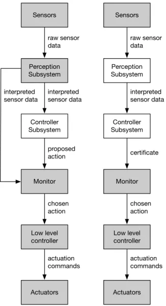
Certified control (Fig. 1-1) is a new architecture that centers on a different kind of monitor. As with a conventional safety architecture, a monitor vets proposed actions emanating from the main controller. But the certified control monitor does not check actions against its own perception of the environment.
Instead, it relies on the main perception and control subsystems to provide a certificate that embodies evidence that the situation is safe for the action at hand. The certificate is designed to be unforgeable, so that even a malicious agent could not convince the monitor that an unsafe situation is safe. The evidence comprises sensor
readings that have been selected to support a safety case in favor of the proposed action; because these sensor readings are only selected by the main perception and control subsystems (and are signed by the sensor units that produced them), they cannot be faked.
A certificate contains the following elements: (1) the proposed action (for example, driving ahead at the current speed); (2) some signed sensor data (for example, a set of LiDAR points or a camera image); (3) optionally, some interpretive data. This data indicates what inference should be drawn from the sensor readings. For example, if the sensor data comprises LiDAR points intended as evidence that the nearest obstacle is at least some distance away, the interpretive data might be that distance; if the sensor data is an image of the road ahead, the interpretive data might be the purported lane lines.
The evidence and interpretive data are evaluated by the certificate checker using a predefined runtime safety case. As an example, consider a certificate that proposes the action to continue to drive ahead using LiDAR data. In this case, the LiDAR points argue that there is no obstacle along the path; each LiDAR reading provides direct physical evidence of an uninterrupted line from the LiDAR unit to the point of reflection. Together, a collection of such readings, covering the cross section of the path ahead with appropriate density, indicates absence of an obstacle larger than a certain size.
Compare this with a classic monitor that interprets the LiDAR unit’s output itself. The LiDAR point cloud is likely to include points that should be filtered out. In snow, for example, there will be reflections from snowflakes. Performing snow filtering would introduce complexity and likely render the monitor unverifiable. On the other hand, a simple monitor would not attempt to identify snow, and could set a low or a high bar on intervention—requiring, say, that 10% or 90% of points in the LiDAR point cloud show reflections within some critical distance. The low bar would result in a monitor that violates soundness, failing, for example, to prevent collision with a motorcycle whose cross section occludes less than the 10% of points. The high bar would result in a monitor that violates honesty, since it would likely cause an
Sensors Controller Subsystem Monitor Actuators actuation commands Perception Subsystem Low level controller raw sensor data interpreted sensor data certificate chosen action Sensors Controller Subsystem Monitor Actuators actuation commands Perception Subsystem Low level controller raw sensor data interpreted sensor data proposed action chosen action interpreted sensor data
Figure 1-1: A conventional runtime monitor (left) and certified control monitor (right). The trusted base is shown in gray.
intervention due to snow even when the road ahead is empty of traffic.
It should be noted that certified control does not remove the sensor and actuator units from the trusted base. What is removed is the main perception and controller subsystems, crucially including complex algorithms that process and interpret sensor readings.
1.2.1
A LiDAR-based Implementation of Certified Control
An implementation of Certified Control was developed to handle this point cloud fil-tration problem. In this implementation, the certificate proposes to continue straight
ahead, using LiDAR points as evidence that there is no impending obstacle. To en-sure the safety of a controller’s decision to move forward, the monitor checks that the points in the certificate have sufficient spread and sufficient density. To achieve sufficient spread, certificate points must horizontally span the size of one lane in front of the car and vertically span the height of a car. Additionally, the monitor checks whether there are any points closer than some minimum forward distance from the car.
The monitor considers the certificate sufficiently vertically dense if it includes points from each of the LiDAR scan rows which fall within the lane. The points are sufficiently horizontally dense if there are no horizontal gaps of a size greater than some pre-specified parameter.
The controller uses radius outlier removal (ROR) filtering, an improvement upon statistical outlier removal (SOR), to identify LiDAR points reflecting off snow [18]. The controller preprocesses the entire LiDAR point cloud into a k-dimensional tree, which it then queries for nearest neighbor information. Points with few neighbors, relative to the average neighborhoods in the point cloud and based on tunable param-eters, are labeled as snow. The controller then constructs the certificate by selecting points from the remaining subset (namely, those not identified as snow) to meet the spread and density criteria.
This monitor’s performance was tested in simulated snowy conditions by dropping confetti-like paper in front of a robot car and confirming that the monitor accepts a certificate when there is sufficient space between the car and an obstacle ahead, despite the presence of simulated snow. When the controller’s filtering parameters were set appropriately, it properly identified points as snow and passed a certificate excluding them to the monitor. Assuming snow was distributed fairly evenly across the lane ahead (and there was not a total “white out”) the remaining points were still sufficiently dense to establish absence of an obstacle in the lane ahead.
The converse case was also tested. Tuning the filtering parameters, or adapt-ing them to the perceived environment, can be difficult. One can imagine even a non-adversarial controller failing to set appropriate parameters, and therefore
mis-categorizing true obstacles as snow. To demonstrate that the monitor would detect such obstacles even when the controller fails to do so, the controller was modified so that it would erroneously filter out some sparse but significant obstacles, such as fallen tree branches (simulated, for the robot car, with plastic cables). As expected, since the controller omitted points on the obstacle from its certificate, the monitor’s horizontal density check failed, rejecting the certificate, and preventing an unsafe action.
1.3
Related Work
The literature on safety assurance of vehicle dynamics splits roughly into two camps, both of which focus on assurance of the planning/control system, and assume per-ception is assured by some other mechanism.
One focuses on numerical analysis of reachable states. For example, reachable set computations can justify conflict resolution algorithms that safely allocate disjoint road areas to traffic participants [19]. The other focuses on deductive proofs of safety. The work of [20] models cars with double integrator dynamics, and uses the theorem prover KeYmaera to prove safety of a highway scenario, including lane changing, with arbitrarily many lanes and arbitrarily many vehicles. The work of [21, 22] demonstrates how these safety constraints can be used for verification and synthesis of control policies, including control policies with switching. In [23], the authors develop safety contracts that include intersections, and provide KeYmaera proofs to demonstrate safety.
Responsibility-Sensitive Safety (RSS) [17] is a framework that assigns responsi-bility for safety maneuvers, and ensures that if every traffic participant meets its responsibilities, no accident will occur. The monitoring of these conditions is con-ducted as the last phase of planning, and is not separated out as a trusted base. The RSS safety criteria have been explored more formally to boost confidence in their validity [24].
reli-able. In contrast, certified control takes the perception subsystem out of the trusted base. Nevertheless, these approaches are synergistic with ours. In our design, the low-level controller is still within the trusted base and would benefit from verifica-tion. RSS provides more sophisticated runtime criteria than those we have considered that could be incorporated into certificates (e.g., for avoiding the risk of collisions with traffic crossing at an intersection).
Several approaches aim, like ours, to establish safety using some kind of monitor. The Simplex Architecture [13, 25], described above, uses two controllers: a verified safety controller and a performance controller. When safety-critical situations are detected, the system switches to the verified controller, but otherwise operates under the performance controller. [26] extends Simplex to neural network-based controllers. As we noted, this approach does not address flaws in perception. In contrast, reason-ableness monitors [27, 28] defend against flawed perception by translating the output of a perception system into relational properties drawn from an ontology that can be checked against reasonableness constraints. This ensures that the perception system does not make nonsensical inferences, such as mailboxes crossing the street, but aims for a less complete safety case than certified control. Similarly, the work of [29] seeks to explain perception results by analyzing regions of an image that influence the per-ception result. These techniques may be useful to enable the perper-ception system to present pixel regions to the safety monitor as evidence of a correct prediction.
Other techniques seek to use the safety specifications to automatically stress test the implementation [30, 31, 32]. A different approach checks runtime scenarios dy-namically against previously executed test suites, generating warnings when the car strays beyond the envelope implicitly defined by those tests [33]. Certified control is similar in that the certificate criteria represent the operational envelope considered by the designers, and outside that envelope, it will likely not be possible to generate a valid certificate, leading to a safety intervention.
Assurance of perception systems needs to grapple with two key challenges. The first is the difficulty of determining appropriate specifications for perception systems, and the second is with developing scalable reasoning techniques to ensure that the
implementation satisfies its specifications. Reasonableness monitors provide a partial answer to the first. The second is an active area of research: [34], [35], and [36], for example, develop efficient techniques to prove that a deep neural network satisfies a logical specification. While these technologies are promising, their applicability to industrial-scale applications has not yet been demonstrated. Perception is a particu-larly thorny problem, since it is not clear what properties of a perception system one would want to formally verify.
1.4
Contributions
The majority of the sections above were taken from a co-authored paper submission on Certified Control[37]. The contributions of this thesis include:
1. an implementation of certified control for visual lane detection; 2. an augmentation of the visual lane detection monitor with LiDAR;
3. a new LiDAR-based monitor incorporating both object position and velocity data;
4. a full visual lane detection system focusing on improving monitor security; 5. the evaluation of these methods with a physical racecar, real driving data, and
in simulation.
The code discussed in the following sections is publicly available at: https://github.com/jefftienchow/Thesis_Code.
Chapter 2
Certified Control with Vision
To explore the application of certified control in the domain of vision, we focused on the verification of lane-line detection. When an autonomous vehicle proposes an action (such as "continue in lane") within the context of the current lane, it must know the current locations of the lane boundaries for the action to be safe. To maintain safety, the controller must provide evidence that the current lane is where it says it is. We designed an application of Certified Control that confirms whether the controller is correctly perceiving the locations of lane boundaries.
2.1
Design
The goal of the monitor is to be able to confirm with high confidence that the con-troller is correctly perceiving the road with relatively low latency. To do so, the monitor must be presented with enough information to make these deductions with-out having to resort to more complicated methods (i.e. machine learning). Thus, the controller is tasked with assembling a certificate containing a set of proposed lane line locations and sufficient metadata that serves as evidence that the proposed lane lines are correct.
This Certified Control implementation is specifically designed to only be applicable to highway-driving situations. Therefore, this may not be robust to residential or less-conventionally marked roads; these conditions may need a different design to work.
2.1.1
Controller
In this scheme, the certificate assembled by the controller contains the following elements:
• the signed image frame from which the lane lines were deduced;
• the left and right lane boundaries given, as second-degree polynomials in the bird’s-eye/top-down view (𝐿(𝑑) and 𝑅(𝑑), respectively), both lines giving the distance from the left side of the top-down view as a function of distance from the front of the car;
• a transformation matrix 𝑇 used to transform the lane points from the bird’s-eye view to the camera view;
• a series of color filtering thresholds used to process the image and highlight the presence of the lane lines.
Depending on performance constraints, the controller may instead incorporate a compressed/downsampled image in the certificate. This can greatly speed up the monitor’s latency. However, if the image is downsampled too much, this can of course come at the cost of accuracy.
2.1.2
Monitor
Using the provided certificate, the monitor verifies performs two tests:
1. a geometric test which checks that the proposed lane lines are geometrically consistent and plausible
2. a conformance test which checks that there are light-colored strips on the road present at the specified locations
In the geometric test, the monitor evaluates the proposed lane lines as a pair; if they conform to specific geometric bounds (such as parallelism) then the lane lines pass this test. The conformance test is a computer vision check. Computer vision
techniques are used to determine whether the proposed lane lines correspond to lane line markings in the image. If they do, the lane lines pass. The proposed lane lines must pass both checks in order for the certificate to be accepted.
Geometric Test
The geometric test ensures that the purported lane lines are parallel and spaced according to local regulations. In the US, for example, the width of a freeway lane is 12 feet [38]. The geometric check is done as follows:
1. The polynomial 𝐿(𝑑) corresponding to the left proposed lane line is sampled at intervals to form a discrete set of points along the line 𝑙 = 𝑙0, 𝑙1, 𝑙2, ..., 𝑙𝑛;
2. For each 𝑙𝑖, we compute the slope of the normal line 𝑛𝑖 to the lane polynomial.
We then find the intersection of the 𝑛𝑖 with the right polynomial 𝑅(𝑑) and
compute the distance 𝑥𝑖 between 𝑙𝑖 and that intersection point;
3. We calculate the standard deviation of the distances 𝑥1, ...𝑥𝑛 and check that it
is below some threshold;
4. We calculate the mean of the distances 𝑥1, ...𝑥𝑛and check that it is within some
delta of the expected distance between lane lines.
In our initial design, we compared the distances between left and right lane lines at various distances from the front of the car to get the average width of the lane and deviation between the lines. However, this does not work well with curved lane lines, as the distance between the left and right lines increase as the lines curve. We fixed this by instead comparing the length of the normals between the lines. Using the normals allows us to evaluate the distance between the lane lines as constant, even when the road curves (Fig. A-1).
The problem of checking the lane width and comparing lane boundaries for par-allelism is greatly simplified by working with a bird’s-eye perspective of the lane boundaries. The transformation and fitting of the lane-lines is done by the main controller, so the checks performed by the monitor remain simple.
(a) Distance measured using horizontal lines (b) Distance measured using normals
Figure 2-1: Measuring distance between the lane lines is more accurate when mea-suring across the normals of the lines.
In the case that lane lines happen to not adhere to local standards, we argue that it is fine for the monitor to intervene. Since it cannot reliably guarantee that rules of a typical road apply in that scenario, it cannot guarantee safety.
Conformance Test
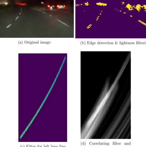
It is not enough to check whether the proposed lane lines have correct geometry, as this only tells us whether the proposed lane lines could be possible. Proposed lane lines might happen to pass the geometric test (or be maliciously tailored to pass it) but not actually correspond to lane lines on the road itself. It is therefore essential to also check that the lane lines conform to a signed image of the road. To do this, the monitor applies simple and well-tested computer vision algorithms to determine if there are corresponding lane markings in the image. The match between the proposed lane lines and the image is checked as follows (Fig. 2-2):
1. The monitor computes the logical OR of the image filtered with an edge detec-tion algorithm on lightness value (such as the Sobel operator) and the image
(a) Original image (b) Edge detection & lightness filtering
(c) Filter for left lane line (d) Correlating filter and left-half of image
filtered by lightness above a certain threshold. These thresholds are computed by the controller and passed to the monitor as part of the certificate.
2. Using the bird’s-eye transformation matrix passed from the controller, the mon-itor transforms the lane lines 𝐿(𝑖) and 𝑅(𝑖) from the bird’s-eye view to the camera’s view.
3. For the transformed left lane curve 𝐿𝑇(𝑖) (and correspondingly for the right),
the monitor creates a filter based on the curve, slightly blurred to allow for some margin of error in the proposed lane lines. The bottom of the filter is weighted more heavily because deviations in the region closest to the car are more important. At points not on the curve, the filter is padded with negative values so that only thin lines that match the filter’s shape will produce a high correlation output.
4. The monitor computes the cross-correlation 𝐶 between the filter and the left side of the processed image (and correspondingly for the right), and finds the point of highest correlation in the image (namely (𝑖max, 𝑗max)such that 𝐶[𝑖max, 𝑗max] =
max(𝐶)). It checks that the point of highest correlation lies within some small distance from the transformed lane line 𝐿(𝑖), and that the maximum correlation is above a predefined threshold.
Once again, we push the complexity of having to determine the specific bird’s-eye transformation to the controller. Since the monitor just accepts the transformation as part of the certificate, it can remain simple while still adapting to the curvature and environment of the road (as the controller does). However, since the monitor does not check the validity of the transformation, the transformation is currently considered as part of the trusted base. A potential solution to this problem would be to once again task the controller with producing a certificate proving the correctness of the suggested transformation and add some check to the monitor to confirm the validity of that transformation. For example, the certificate could also include LiDAR points on the ground, and the monitor (which now has the exact coordinates of those
LiDAR points) could create a two-dimensional projection of those points from both the camera view and the bird’s-eye view. The monitor could then check whether the transformation matrix accurately maps points from the bird’s-eye view to the camera view.
Originally, the certificate was composed of the lines in the camera view and a transformation from the camera view to the bird’s-eye view. This was beneficial because it allowed us to distinguish between dotted and solid lane lines. If we look at images from the bird’s-eye view, the space between dots on a dotted lane line are more consistent (whereas for images in the camera’s view, spaces between those dots are larger closer to the vehicle); therefore, we were able to create separate filters for dotted and solid lane lines. However, openpilot, our vision controller of choice that is discussed in the next section, already internally computes a camera view to bird’s-eye view transformation matrix, so we decided to use that in our certificate to reduce project complexity.
2.2
Experiments
The vision certificate checking scheme was implemented and evaluated against two different lane-detection software systems. While tweaking parameters, our primary goals were to eliminate the false positives (the monitor rejecting the certificate when the suggested lane lines are accurate) and the false negatives (the monitor passing the certificate when the suggested lane lines are inaccurate). In addition, we primarily focused on highway conditions, as this certified control implementation is not designed to work on non-highway conditions.
2.2.1
Openpilot Implementation
The first lane-detection system we tested our design with was openpilot [39], an open source production driver assistance system that can be used to control and drive vehicles. We used real replay data from a car driven using the system. In particular, we ran our monitor using the Comma2k19 dataset [40], which includes
Figure 2-3: An example of a lane-detection failure detected by the monitor. The green lines represent the proposed lane lines.
driving segments with non-highway driving and adverse lighting conditions (such as a rainy night).
Openpilot’s implementation exposes a few variables that allows for easy integration into our monitor implementation. In particular, it exposes:
1. Points on the left and right lane lines in the image in the bird’s-eye view. 2. The image used to deduce the location of the lane lines.
3. A transformation matrix that can be used to transform the lane lines points to the camera view.
Since openpilot uses a complex neural network to do its lane-finding, there were not any color-filtering thresholds readily available to incorporate into the certificate. Instead, we configured openpilot to pass in a predefined set of thresholds to the monitor to use in its check.
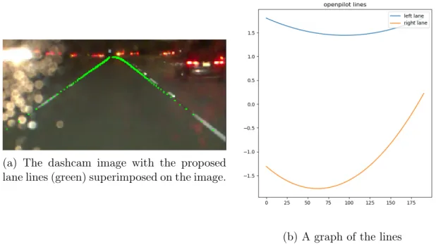
In several instances, our monitor caught lane detection failures (Fig. 2-3). In all failure cases, however, openpilot was able to successfully correct its lane detection within a few seconds. For some of these cases, it was not obvious from inspection of the image taken from the camera’s perspective that the proposed lane lines were not
(a) The dashcam image with the proposed lane lines (green) superimposed on the image.
(b) A graph of the lines
Figure 2-4: The lane-lines looks plausible from the camera’s view, but further away, the lines are not parallel; this can more easily been seen from the bird’s-eye view. geometrically correct. However, viewing from the bird’s-eye perspective, it was easier to see that they could not correspond to plausible lane lines (Fig. 2-4). See Fig. 2-5 for more examples of passing and failing lane lines.
2.2.2
Racecar Implementation
The second experiment was conducted with a physical racecar. We implemented a naive lane-detection scheme to serve as the controller, which deduced lane lines through the following steps:
1. The image from the racecar’s camera is converted to a hue, saturation, value (HSV) image to allow for easier segmentation based on lightness values.
2. Upper and lower HSV color thresholds are used to segment the the image into a mask for the blue portions of the image.
3. Noise is removed using an erosion filter.
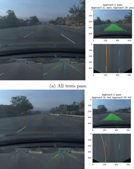
(a) All tests pass.
(b) Lane lines pass the geometric test but correctly fail both conformance tests.
(c) Conformance test also works under darker lighting conditions with rain.
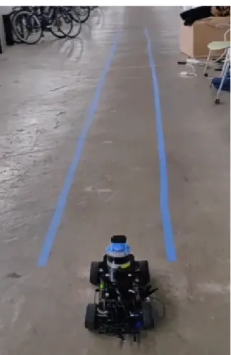
Figure 2-6: The setup of the racecar with blue tape representing lane lines. 5. The lines are separated into two groups based on slope. Due to the camera’s
perspective, a positive slope corresponds to a left lane line and a negative slope corresponds to a right lane line.
6. The lines in each group are averaged to produce an estimate of the locations of the left and right lane lines. These lines are represented as first-degree polyno-mials.
To simulate potential lane lines, we placed blue tape on the floor in front of the racecar (Fig. 2-6). When we tested the monitor with only straight and parallel lane lines, the monitor never rejected the certificate given from the controller. However, when we placed additional tape segments in inappropriate positions, we were able to get the lane detector to report bad lane lines (Fig. 2-7); in all cases, the monitor correctly rejected them.
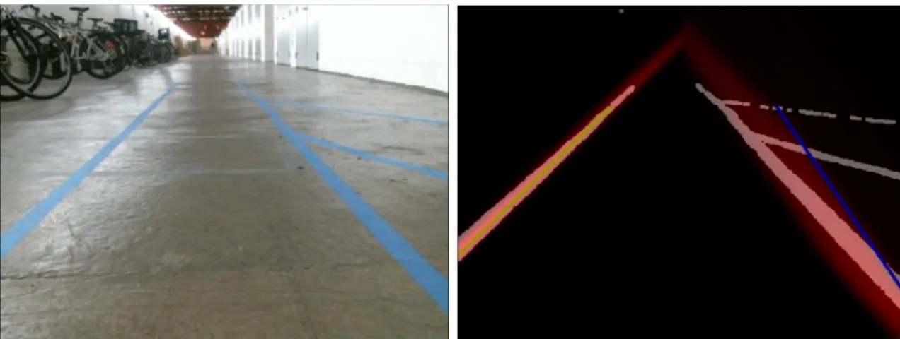
(a) Additional blue tape is placed on the right side to cause the naive controller to propose bad lines.
(b) The proposed right lane line (blue) fails because the correlation (red) at points along the proposed line is not strong enough.
Figure 2-7: The monitor correctly rejects lane lines when the controller proposes incorrect lane lines due to the additional blue tape.
Component Lines of Code
Vision Monitors library calls 90 Vision Monitors self-written code 235
Vision Monitors Total 325
Controller library calls 460
Controller self-written driver code 612
Vision Controller Total 1072
Figure 2-8: Comparison of code sizes for the monitor vs. certificate generation within the controller. Only the racecar code is included; the openpilot version uses a complex neural network.
2.3
Evaluation
Both implementations of the vision monitor were able to correctly detect errors in lane-finding controllers. Neither controller, however, had the capability of generating variable color filtering thresholds (depending on lighting conditions) to incorporate in the certificate. The motivation for including these thresholds in the certificate was to allow the monitor to adapt to different lighting conditions since lighting can potentially affect whether the monitor verifies a certificate. See Appendix A for an experiment demonstrating how varied color thresholds can improve the monitor’s accuracy under adverse lighting conditions.
Overall, even though the racecar used only a naive lane-finding algorithm with no machine learning, the algorithms still used three times as many lines of code as the monitor’s three vision checks combined (Fig. 2-8). Production controllers are of course much more complex—openpilot’s deep learning container for lane-finding on github has around 26 convolutional and 7 fully connected layers.
The certificate used for openpilot required about 45KB of storage, dominated by the image. On average, checking of the certificate took about 0.08 seconds on a Dell XPS 9570 Intel Core i7-8750H CPU with 16GB RAM. We achieved this latency and certificate size by downsampling the image by a factor of 2. This may not be adequate performance in a production system, but it is within an order of magnitude of what would be required. With proper optimization of the checking algorithm, and some additional compression of the image, performance seems unlikely to be a problem.
2.4
Limitations
2.4.1
Using Visual Data
This certificate is inherently less trustworthy than the LiDAR certificate. This seems unavoidable, since unlike the physical obstacles detected by the LiDAR scheme, a single pixel does not tell much about what is present at a particular location. Vi-sual data generally must be interpreted at a larger scale (than just a single pixel), introducing more complexity. In addition, following lane lines is a social convention, with the lane lines acting as signs whose interpretation is not a matter of straightfor-ward physical properties. Therefore, it may be necessary to use more sophisticated methods to confirm the locations of lane lines when the lines are only implied by the presence of these conventions as opposed to the presence of light-colored bands on the road.
2.4.2
Obstructed/Unclear Lane Markings
This implementation assumes that both the left and right lane lines are fully visible and therefore does not work with partially (or fully) occluded lane lines. There are
Figure 2-9: A frame that caused the conformance test to fail due to the faded right-hand lane line.
two failure cases that we encountered during testing. The first involves obstructed lane lines. Our design assumes that the lane boundaries are always at least partially visible. Since the Comma2k19 dataset includes segments with non-highway driving, there were cases in which multiple cars were lined up at a stoplight and obscuring the lane lines. On the highway, the lane lines could be similarly obstructed during traffic or when a car in front is changing lanes. It is possible that more sophisticated methods would be needed to address these cases. The second failure case involves poorly painted lane lines. In one case, a lane line was so faded it caused the correla-tion output of the conformance test to not reach the desired threshold and therefore fail the check (Fig. 2-9). This situation could be mitigated if color filter thresholds were dynamically computed and passed by the controller to the monitor. However, since such thresholds were not exposed in openpilot, we passed constant values to the monitor. This failure case also reflects the fact that compelling evidence of the presence of a lane will require well-drawn lane lines; a successful deployment of au-tonomous cars might simply require higher standards of road markings. It is essential to realize that certified control does not create or even exacerbate this problem but merely exposes it. If the designer of an autonomous vehicle were willing to rely on
inferring lanes from poorly drawn lines, the certificate requirements could be reduced accordingly, so that the level of confidence granted by the certificate reflect the less risk-averse choice of the designer.
Another concern with the current implementation is the use of conventional edge detection algorithms. The current implementation fails to confirm lane lines when the road is poorly lit (ex: trees casting shadows on the lane lines). This is a known problem with the Sobel operator, but can potentially be fixed using better edge detection algorithms [41].
2.4.3
Lack of Time-Domain Awareness
This implementation does not store any metadata or results from previous timesteps. The previous limitations discussed could potentially be resolved if the monitor ob-served how lane lines and images change over time. For example, if a lane line is present in one frame and occluded in the next, one might infer that the lane line is still there but just concealed in that frame. This could potentially eliminate some incorrect interventions from the monitor, as the monitor would be more robust to sudden changes in lane visibility.
On the other hand, utilizing temporal data would increase the complexity of the monitor and would lead to a larger trusted base. A potential solution would be to only have the controller include temporal data when necessary (e.g., when a lane line is occluded) and incorporate past frames as evidence that there is likely still a lane line present at the specified location.
Chapter 3
Combining Vision with LiDAR
3.1
Motivation
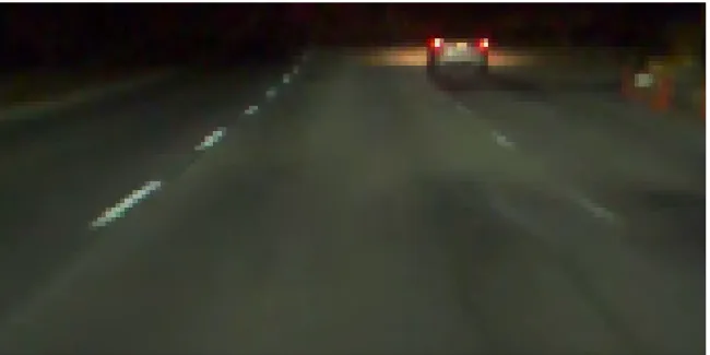
Image data lacks the inherent physical properties of LiDAR data: a single pixel, unlike a single LiDAR point, says nothing about the car’s environment, absent other context. As a result, one can only perform limited checks on the lane lines using vision alone. In a particular case involving a Tesla driving with autopilot, the vehicle almost crashed into a concrete barrier. The problem was that bright lines that look similar to lane lines appeared on the barrier in the camera’s image [42]. These lines were actually bands of direct or reflected sunlight. In most cases, we believe that the vision tests described above would catch such anomalies; we took one particular image from an online video (Fig. 3-1) illustrating this problem and confirmed that the inferred lane lines would indeed fail the geometric test and be correctly rejected. However, it is conceivable that these spurious lane lines would have passed the geometry and conformance tests. Indeed, in the Tesla example, the yellow ray of sun almost looked, in the image, like a plausible lane line. Apparently a more basic property is being violated: the detected lane line is on the barrier and not on the ground.
This motivates a certificate that integrates LiDAR and vision data for verifying lane line detection. In addition to providing the lane line polynomials and the camera image (as above), the certificate also provides a set of LiDAR points that lie on the
Figure 3-1: An image taken from dashcam footage in which a car using Tesla’s au-topilot almost ran into a concrete barrier. The malfunction was presumably caused by the perception system mistaking the reflection along the barrier for a lane line. purported lane lines. The monitor checks that these LiDAR points indeed correspond to the lane lines and that they reside on the ground plane. The controller, as usual, is given the more complex task: finding that ground plane and selecting the LiDAR points.
3.2
Design
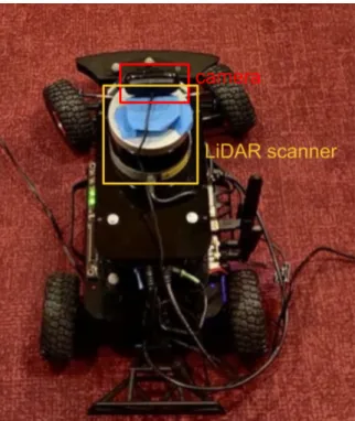
After the controller computes the location of the lane lines on the image, it is re-sponsible for determining the LiDAR points that correspond to those lane lines. The controller does this by sampling points along the lane line polynomial and transform-ing them into 3D space. We assume that the camera and the LiDAR scanner are both at the same location, which is approximately true given our setup (Fig. 3-2). We also assume we are working with a pinhole camera, allowing us to use the pinhole camera model to relate the 3D location of objects to their 2D projection. To determine which pixels along the lane lines to sample, we utilize the vertical angle of the LiDAR rows given by the LiDAR scanner specifications. This is to prevent us from choosing pixels on the image that lie in between LiDAR rows (which would naturally not correspond to any scanned LiDAR points). For each row with a vertical angle corresponding to a pixel below 1/3 the height of the image, we sample one point for each of the lane lines.
Figure 3-2: Our racecar setup, with the camera mounted directly above the LiDAR scanner.
Given a point (𝑥, 𝑦) in our 2D image sampled in this way, we can simply search that corresponding LiDAR row to find the point that most closely matches the horizontal angle of the pixel, telling us approximately which LiDAR point corresponds with that pixel.
We additionally task the controller with identifying a ground plane. Our con-troller implementation runs a random sample consensus (RANSAC) algorithm [43], augmented with some constraints. More specifically, the controller uses additional heuristics to make sure that the proposed ground plane is plausible. For example, the controller requires that the ground plane lies below the camera and that the plane is sufficiently flat.
Given the LiDAR lane line points and the ground plane, the monitor checks that: • the proposed LiDAR points indeed match the proposed lane lines. This is again
done using trigonometric methods;
• the proposed LiDAR points are sufficiently close to the ground plane; • the ground plane is sufficiently low-lying (below the camera) and flat;
(a) Image taken from the camera on the race-car showing the sampled points (red) corre-sponding to the LiDAR rows.
(b) The same setup from a higher perspec-tive.
Figure 3-3: The lines look plausible from a 2D perspective, but the right line is not on the ground. The red dots on the lines in (a) are the points sampled along the line that lie at the same angles as the LiDAR scanner rows.
• there is a high enough density of points lying close to the ground plane.
3.3
Experiment
To simulate the Tesla barrier malfunction, we lined up two rows of tape to look like lane lines (Fig. 4-1). The tape for the left line was placed on the ground while the tape for the right lane was elevated on a platform; from the camera’s perspective, the pair of lane lines looked geometrically plausible. When we ran our combined vision-LiDAR implementation on this scenario, the monitor correctly rejected the certificate because the points from the right lane line were not on the ground plane. This check would theoretically also detect false lane lines which lie above or below the ground plane for any other reason.
3.4
Evaluation
The integration of vision with LiDAR presents a few unique challenges. First, the ground plane detector we implemented is not robust to steeply sloped roads or to very uneven road surfaces. Our RANSAC algorithm only finds flat planes, so the controller cannot yet propose curved planes. However, improving the system to work with those conditions would mean only a more complex controller–the monitor need not become more complex. Second, since the monitor’s checks to determine the validity of the ground plane are not exhaustive, it is possible the monitor would not detect a false ground plane. This is partly because the controller does not include in its certificate any proof of validity of the ground plane it detected, and thus, the ground plane algorithm must be regarded as within the trusted base. The obvious remedy—namely including the ground plane detection in the monitor—is not straightforward for two reasons: the algorithm is too complex to be easily verifiable, and the monitor only has access to the points in the certificate, not the entire LiDAR point cloud. Nevertheless, this could potentially be solved with our usual approach: by tasking the controller with producing a certificate which proves to the monitor the validity of its suggested ground plane, e.g. by inclusion of certain low-lying points.
Chapter 4
Enhancing the LiDAR Monitor
The original LiDAR-based implementation of certified control establishes that the LiDAR points have sufficient spread and density and verifies that there are no points within some minimum forward distance from the ego vehicle. In other words, the monitor determines whether or not the controller is filtering out too many points and intervenes if there are obstacles closer than some set distance from the front of the car. In reality, some objects can be closer to the ego vehicle while maintaining safety and others must be further away. More specifically, danger of collision also depends on the velocity of objects relative to the ego vehicle. For example, if the ego vehicle is driving at 20m/s and an object is 5m in front of the ego vehicle, the safety of the situation depends on how fast that object is moving. If it is stationary, then the ego vehicle might crash into it; if it’s also moving forward at 20m/s, then the situation is probably not dangerous.
4.1
Design
Similar to the original LiDAR certificate, the controller is tasked with taking the LiDAR point cloud and filtering out noise (such as snowflakes) while keeping the points dense and spread out enough to ensure no large objects are filtered out. As of now, the controller is only tasked with passing points in front of the ego vehicle to the monitor. In addition, the LiDAR points now include a velocity in addition
to a position; this velocity corresponds to the speed of the particle that reflected the LiDAR point relative to the ego vehicle. We assume there is some method of obtaining the relative velocity of a LiDAR point. For example, LiDAR technology has the ability to discern the speed of objects using the Doppler Effect with high accuracy [44]. These position-velocity pairs are passed to the monitor to determine whether the proposed velocity of the ego vehicle is safe.
Similar to the previous design, the monitor checks for sufficient density and spread within the LiDAR points, confirming that there are no large areas in the ego vehicle’s lane that do not contain LiDAR points. The monitor also evaluates each point in the certificate by checking whether it’s possible for the ego vehicle to collide with the point, assuming that the ego vehicle continues straight at the suggested velocity. To perform this calculation, we will work within a one-dimensional framework where we only care about object velocities in the forward direction.
4.1.1
Case 1: Objects Don’t Move Backwards
We first handle the case where objects in front of the car will not move backwards toward the ego vehicle. We assume that the maximum deceleration 𝛽𝑚𝑎𝑥 an object
can have is 9𝑚/𝑠2, an estimate from a study on emergency braking capabilities of
vehicles [45]. We argue that this is acceptable because objects on the road are not likely to have a higher maximum deceleration than a car. Given these assumptions, the worst case for the ego vehicle would be if all other objects were to suddenly decelerate at 𝛽𝑚𝑎𝑥, as this would be the situation that brings objects as close to the
colliding with the ego vehicle as possible. Since we are assuming objects can have a maximum deceleration of 𝛽𝑚𝑎𝑥, objects that have lower deceleration rates would end
up further in front of the ego vehicle; using 𝛽𝑚𝑎𝑥 for all points gives us a conservative
worst-case estimate of where points could end up in the near future.
If the ego vehicle were to approach an unsafe scenario where it might crash into an upcoming obstacle, we also want to give the controller time to circumvent the danger. Thus, we can determine whether we need to intervene by calculating whether the ego vehicle will crash into any objects decelerating at 𝛽𝑚𝑎𝑥 given that the ego vehicle
is also decelerating at its maximum deceleration rate 𝛽𝑒𝑔𝑜𝑚𝑎𝑥. In other words, we
assume that the controller will drive safely until the last possible moment: when braking at the ego vehicle’s maximum deceleration will just barely cause a collision with a particle decelerating at 𝛽𝑚𝑎𝑥.
We compute the position of the ego vehicle if it were to fully brake and compare that position to the location of objects if they were to decelerate at 𝛽𝑚𝑎𝑥 toward the
ego vehicle. If the ego vehicle is in front of an object, there must have been a collision. See Appendix B for our reasoning.
To calculate the braking distance of the ego vehicle, we also need to consider the latency from when the monitor sends the command to when the actuator brakes. Taking this into account, we get a formula for determining when to intervene:
𝑣2 𝑒𝑔𝑜 2𝛽𝑒𝑔𝑜𝑚𝑎𝑥 + 𝜌 · 𝑣𝑒𝑔𝑜> 𝑑 + 𝑣2 𝑓 2𝛽𝑚𝑎𝑥 where
• 𝑣𝑒𝑔𝑜 is the forward velocity of the ego vehicle;
• 𝛽𝑒𝑔𝑜𝑚𝑎𝑥 is the maximum deceleration capability of the ego vehicle;
• 𝜌 is the latency between messages going from the monitor to the actuators; • 𝑑 is the forward distance between the front of the ego vehicle and the object in
question;
• 𝑣𝑓 is the forward velocity of the object in question;
• 𝛽𝑚𝑎𝑥is the maximum deceleration capability of the object, assumed to be 9𝑚/𝑠2.
4.1.2
Case 2: Objects Move Backwards
To handle cases where objects are moving backwards towards the ego vehicle (ex: a tire that comes off a car), using the assumption that objects are going to have a deceleration of 𝛽𝑚𝑎𝑥no longer leaves us with a worse-case analysis. On the other hand,
assuming objects will accelerate towards the ego vehicle is also not a good assumption; if we were to assume objects on the road were to accelerate toward the ego vehicle, it
would be impossible to share the road with other objects/vehicles. Thus, we assume that objects moving backwards will continue at their current velocity, giving us a more reasonable worst-case analysis.
This poses the question, how long do we assume the object will move backwards? Since the monitor only has the power to stop the ego vehicle, and putting the ego vehicle in reverse would complicate matters much more, we will again assume that the best course of action in a dangerous situation is to maximally decelerate the ego vehicle. Therefore, we only need to analyze how far objects will move backwards in the time it takes the ego vehicle to fully stop. If the object continues to move toward the ego vehicle even after the ego vehicle has completely stopped, then the monitor could not have prevented the collision (at least with only the power to actuate the brakes).
Therefore, we can summarize whether or not the monitor should intervene with the following formula that considers the worst result of the two above cases:
𝑣2 𝑒𝑔𝑜 2𝛽𝑒𝑔𝑜𝑚𝑎𝑥 + 𝜌 · 𝑣𝑒𝑔𝑜> min(𝑑 + 𝑣𝑓2 2𝛽𝑚𝑎𝑥, 𝑑 + 𝑣𝑓 · 𝑡𝑠𝑡𝑜𝑝) where • 𝑑 + 𝑣𝑓2
2𝛽𝑚𝑎𝑥 is the distance between the ego vehicle and an object if it decelerates
at 𝛽𝑚𝑎𝑥;
• 𝑑 + 𝑣𝑓· 𝑡𝑠𝑡𝑜𝑝 is the distance between the ego vehicle and an object if it continues
at 𝑣𝑓;
• 𝑡𝑠𝑡𝑜𝑝 is the time needed to fully stop the ego vehicle, given by: 𝑣𝑒𝑔𝑜
𝛽𝑒𝑔𝑜𝑚𝑎𝑥 + 𝜌.
Similar to the previous LiDAR monitor implementation, noisy points that do not represent large obstacles that would otherwise cause the certificate to fail should be filtered out by the controller. This greatly simplifies the monitor, as it therefore does not need to do any object segmentation to figure out whether objects in the point cloud are small enough to be ignored.
The monitor evaluates every point in the certificate (using their respective position and velocity) to determine if the vehicle is continuing at a safe speed. If all points
are safe, and there is sufficient spread and density within the ego vehicle’s lane (as in the previous monitor implementation), the certificate passes.
4.2
Implementation
We tested this certified control implementation in CARLA, an open-source vehicle simulation program [46]. CARLA has the ability to spawn and simulate objects in a 3D environment and was developed for the purpose of testing autonomous vehicles. The program comes with a variety of preset maps, environmental conditions, and actors (anything that plays a role in the simulation or can be moved around) which greatly facilitated development. We ran CARLA on Dell XPS15 9500 laptops with 16GB of RAM, an NVIDIA GTX 1650Ti dedicated graphics card, and an Intel i7-10750H CPU.
To implement our certificate design and monitor in CARLA, we took the following steps:
1. Create a world in synchronous mode to allow for full control of the speed of timesteps in simulation. We set the simulated time between ticks to be .05 seconds.
2. Spawn the ego vehicle on the map.
3. Mount a LiDAR object on the ego vehicle set to rotate 10 times per second. Since the LiDAR only completes a full rotation every two timesteps, the con-troller only passes a certificate to the monitor every two timesteps.
4. When a full rotation is completed, filter the LiDAR points for points in front of the LiDAR scanner, above a certain height (1.2m below LiDAR scanner), and within a given left/right boundary (2m, or half the width of a lane).
5. For each of the remaining points, if they are within the bounding box of an actor (person, vehicle, etc), attach the velocity for that actor to that point. If a point is not within the bounding box for an actor, assign it a velocity of 0. This