Analysis of hot-carrier AC lifetime model for MOSFET

(1)

Analysis of Hot-Carrier AC Lifetime Model for

MOSFET

by

Beniyam Menberu

Submitted to the Department of Electrical Engineering and Computer Science in partial fulfillment of the requirements for the degree of

Master of Engineering in Electrical Engineering and Computer Science

at the

MASSACHUSETTS INSTITUTE OF TECHNOLOGY

February 15, 1996

© 1996 Beniyam Menberu. All Rights Reserved.

The author hereby grants to M.I.T. permission to reproduce distribute publicly paper and electronic copies of this thesis

and to grant others the right to do so.

A

uthor ...

... ... ...

~..

Department of Electrical Engineering and Computer Science

January 29, 1996

Certified by ... . ...

...

.

...

James Chung

Associate Professor of Electrical Engineering

Thesis Supervisor

A ccepted by

...

*

F. R. Morgenthaler

Chairman. Department Viwmittee on Graduate Theses

OF TECHNOLOGY

JUN

1

1 1996

(2)

ACKNOWLEDGMENT

I would like to thank my research advisor, Professor James Chung, for his support

throughout the span of my research work. I am also thankful for his guidance that has made a difference on me. I am very proud to have worked for one of the most hard work-ing and intelligent person I have known.

I would also like to thank my fellow research members Abraham Kim, Wenjie Jiang,

Huy Le, Brian Stine, Jee-Hoon Y. Krska, Jung U. Yoon, and Rajesh Divecha. I am grateful for all the support and guidance I received from Abraham Kim and Wenjie Jiang. I would also like to appreciate Brian, Huy, Jee-Hoon, Jung and Rajesh for the help they have given me throughout my research.

My father, Menberu Yemata, has always been the closest person to me throughout

my life. I would like to thank him for all the love he has given to me. My only wish was that my mother would have been here to have seen my accomplishments. May her soul rest in peace. I am also grateful for my brother Dawit, and my sisters Hiwot and Kidist for their support.

(3)

Analysis of Hot-Carrier AC Lifetime Model for MOSFET

by

Beniyam Menberu Submitted to the

Department of Electrical Engineering and Computer Science on January 29, 1996

In partial fulfillment of the requirements for the degree of Master of Engineering in Electrical Engineering and Computer Science

Abstract

This study presents a new algorithm for the prediction of AC hot-carrier lifetime/degrada-tion of NMOSFETs. The hot-carrier degradalifetime/degrada-tion model parameters used in this study were modeled as a quadratic function of the oxide electric field. The new algorithm models the non-linear behavior of the AC hot-carrier degradation accurately using the method of the dominant degradation asymptote. The formulation of the dominant degradation asymptote will be described. Circuit examples are shown to illustrate that the new algorithm is better than the current method in predicting AC hot-carrier degradation. The current method is also shown to overestimate AC lifetime significantly compared to the new algorithm. Thesis Supervisor: James Chung

(4)

List of Figures

Figure 1.1: The current neff method of calculating AC degradation ... 9

Figure 1.2: Determining AC degradation based on identifying the dominant degradation as-ym ptote ... 11

Figure 2.1: Substrate current generation in MOSFETs ... 13

Figure 2.2: Numerical integration of the function A(t)... ... 17

Figure 2.3: DC degradation displaying different n coefficients ... 18

Figure 2.4: Extracting the parameters m and H ... 20

Figure 2.5: Bias dependencies of degradation parameters m, n ... 21

Figure 3.1: DC stress conditions for the two-step waveform ... 27

Figure 3.2: Degradation simulation for two-step waveform...28

Figure 3.3: Asymptotic behavior of the two-step degradation equation...29

Figure 3.4: One-stage inverter with load CL... 30

Figure 3.5: Degradation simulation for an inverter.(W/CL=400um/pF , a = 10-K) ... 30

ns Figure 3.6: Degradation simulation for inverter(N=2xl08cycles)...31

Figure 3.7: Degradation rate n as a function of number of data points used for fitting .34 Figure 4.1: Degradation rate n vs. time(t)... ... 39

Figure 4.2: Instantaneous AGE versus time(t)...39

Figure 4.3: Cumulative AGE versus time(t) ... 40

Figure 4.4: n versus cumulative AGE(semilog plot) ... ...41

Figure 4.5: n versus cumulative AGE(linear scale) ... ... 42

Figure 4.6: Identifying the dominant asymptote...43

(7)

Figure 4.8: Two-step simulation along with current neff and new model ... 46

Figure 4.9: Demonstration of the algorithm for an inverter...47

Figure 4.10: Structure of the new model ... ... 50

Figure 5.1: Ratios rl and r2 for the two-step example ... 58

Figure 6.1: Simulation result for NMOS in inverter( = 400-m, a = 10 V )...59

C pF ns Figure 6.2: Simulation result for NMOS in inverter( a = 1 10m)...60

ns C pF Figure 6.3: Overestimation of lifetime using the current neff method...61

Figure 6.4: Ratio of AC lifetime predicted by the current neff and new method based on dominant asymptotes... ... ... 62

(8)

List of Tables

(9)

Chapter 1 Introduction

1.1 Overview of Hot-Carrier Effects

Hot-carrier degradation is the result of physical mechanisms that are present in MOS-FETs undergoing voltage stress. The electric field at the drain side, Ed, is the driving force for hot-carrier degradation. Because of the high electric field at the drain side, the mobile electrons in the conducting channel of a MOSFET gain high energy as they approach the drain side. These electrons with high energy can break Si-H bonds near the Si/SiO2

face at the drain side which can result in the outward diffusion of hydrogen from the inter-face[1]. This bond breaking can result in the generation of interface traps that can have a detrimental effect on MOSFET performance.

As the dimensions of MOSFETs become smaller and smaller, the issue of hot-carrier reliability becomes a major concern for circuit designers. The presence of hot-carriers in MOSFETs results in device performance degradation. Interface trap generation ANvit

results in change of the threshold voltage AVT, and reduction of the MOSFET drain

cur-AId

rent - and transconductance Ag_m[1]. These changes in device performance can affect Ido

overall circuit performance.

1.2 AC Hot-carrier Circuit Degradation

For AC waveforms, the quasi-static approximation is used to predict the MOSFET degradation/lifetime. The AC waveforms are partitioned in time by small time-steps such that DC conditions apply within each time-step. The quasi-static approximation enables the use of the DC degradation model within each timestep in order to predict AC degrada-tion.

(10)

The DC hot-carrier degradation model is defined by three parameters m,n,H. The parameter n is the degradation rate. The parameter m is the voltage acceleration factor and

H is a process dependent constant. These model parameters can be extracted from drain

AId

current reduction (-) measurements and the corresponding lifetime I: of MOSFETs

do

stressed at different DC bias voltages. The quasi-static approximation predicts AC degra-dation accurately if the AC waveform does not change too rapidly.

Using the quasi-static approximation, the AC lifetime can be calculated at a future time point using an iterative set of equations. However the drawback in using the iterative equations is that it can become computationally infeasible to calculate AC lifetime if the time point of interest is much greater than the period of the AC waveform. For example, it may take years to calculate the AC degradation of a device stressed for only several sec-onds of AC operation (which correspsec-onds to billions of waveform cycles) using the itera-tive equations. Therefore there is a need for an accurate AC hot-carrier degradation model that is not CPU-time extensive.

1.3 Current Method for AC Hot-carrier Degradation

The current AC lifetime prediction method used by BERT(Berkeley Reliability Tools) predicts AC degradation by extrapolation from the first few simulated data points. These simulation data points are obtained by using the exact AC iterative equation. This current

neff methodology is shown in Figure 1.1. Simulation results from the first two AC

wave-form cycles are used to determine the AC degradation model parameters neff and Aeff that define the line shown in Figure 1.1. The AC degradation at a future time point can then be found by extrapolating the line to the future time point of interest.

Usually the future time-point of interest is on the order of 1016 cycles and using only the first two cycles to extrapolate to 1016 cycles can result in huge extrapolation errors.

(11)

This extrapolation error is introduced because the AC degradation can exhibit a complex power-law time dependence.

S-tr df)TI 0#-0

SdO,

_{nff Method}

*

oifextrapolation

neff AId N ,, ln nff

I

rI

d

I I 1 2

Number of Cycles (N)

Figure 1.1 The current neff method of calculating AC degradation.

1.4 Proposed New Method for AC Hot-carrier Degradation

For typical digital circuits, Vgd (gate-to-drain bias voltage) of the pull-down NMOS transistor can vary from

+Vdd

to 0 during transitions of the input signal. Since the degra-dation rate n has significant bias dependency on the oxide-electric field EOO Vgd[4],

modeling the degradation with just a single degradation rate n=neff(such as used in the current neff method) can lead to significant underestimation of the AC degradation or overestimation of the AC lifetime. Therefore, the proposed new method models AC deg-radation using more than a single degdeg-radation rate n. The new method uses the concept of the "dominant" degradation asymptote. Using the quasi-static approximation, the degrada-tion rate n can be calculated at each time step as a funcdegrada-tion of the drain and gate voltage. A

(12)

series of averaged values of n(weighted by the instantaneous age) and the AGE(the cumu-lative value of the instantaneous AGE) calculated from the NMOS voltage waveforms are used to determine the AC degradation asymptote. The new method uses these AC degra-dation asymptotes to give an accurate lower-bound on the AC degradegra-dation at any specified future time-point.

In Figure 1.2, the method of the dominant degradation asymptote is demonstrated schematically. The true AC degradation(determined by the AC iterative equation) can be approximated as a "superposition" of different DC asymptotes. At the particular time point of interest, which in this case is 10 years, the asymptote that predicts the highest deg-radation has to be identified. This asymptote is defined as the dominant asymptote. An ini-tial asymptote in Figure 1.2 is defined by two variables AGET and nave where nave is the average n weighted by the instantaneous age. The asymptotes labeled B & C from Figure 1.2 are then generated from the asymptote labeled A by using nave to partition the initial asymptote A. According to Figure 1.2, asymptote B is more dominant than asymptote A at 10 years since it predicts higher degradation. This asymptote generation process is contin-ued until the most dominant asymptote has been identified.

In terms of computational efficiency, both the new method and the current neff method require significantly less CPU time than the iterative method of predicting AC degrada-tion. However the new method of lifetime prediction, based on dominant asymptotes, takes into account the dynamic behavior of the degradation equation. The new method adjusts to the behavior of the AC degradation by finding the dominant asymptote that accurately bounds the AC degradation at the specified time point. In contrast, only a single degradation rate n is used to predict AC degradation for all times with the current neff methodology[2]. Thus the new method can predict AC degradation with more accuracy.

(13)

Id NT]

Id

dominant

A

(number of cycles) Figure 1.2 Determining AC degradation based on identifying the dominant degradation

(14)

(15)

Chapter 2 DC Hot-carrier Degradation Model

2.1 The Substrate Current Model

Hot-carrier degradation in NMOSFET devices has been shown to correlate very well with substrate current, Isub[2]. Thus Isub can be used as a good monitor for device-level degradation due to hot-carriers. The generation of Isub is the result of the lateral electric field present at the drain side of the MOSFET [2]. Electrons along the channel gain high enough energy from the lateral electric field to cause impact ionization near the drain. The impact ionization results in the formation of electron-hole pairs. The substrate current is the hole current generated when the holes created by the impact ionization are attracted toward the substrate by the repelling electric field. A more complete model of the sub-strate current generation is shown in Figure 2.1 [2] with different arrows representing hole and electron currents. The hole currents in Figure 2.1 make up the substrate current.

GATE

Ionization I

Isub

Substrate

E

Figure 2.1: Substrate current generation in MOSFETs

(16)

The substrate current (Isub) is a function of the drain current Id and a few other param-eters that can be extracted from drain and substrate current data. A general equation for

the hot-electron induced substrate current is[l]:

(p_i

qhE

Isub = Cide (2.1)

where C is a process-dependent parameter, the variable <p, is the critical energy for impact ionization, X is the mean free path for electrons, and Em is the maximum electric field at the drain[l]. The substrate current model is[3]:

-Bil

(Ai

(d7 ~dsatI

Isub = (i)d Vds Vdsat) e Vd-Vda(2.2)

Bi ( _(2.2)

where Vds is the drain to source voltage and Vdsat is as follows[3]:

dsat EcriL (VS -VT) (2.3)

dst - _{critL +} _(Vg

s - VT)

The parameters A_iand B_iare the impact ionization coefficients, Vdsat is the drain satu-ration voltage, and VT is the threshold voltage. For long channel MOSFETs, the Vdsat reduces to the familiar equation Vdsat = Vgs-VT. The parameter l, which is the length of the "effective pinch-off" region [3] of the channel, can be approximated as follows[9]:

1= tx (2.4)

where tox is the gate-oxide thickness and xj is the junction depth of the MOSFET. Ecrit is

the critical field for velocity saturation[3].

2.2 Hot-electron Generation in MOSFETs

Hot-electron degradation is caused by electrons which have high enough energy to break Si-H bonds at the Si/SiO2 interface[1]. This results in the generation of interface

(17)

traps at the Si/SiO2 interface which can cause reduction in the MOSFET drain current,

transconductance, and shifts in the MOSFET threshold voltage. Linear region drain cur-rent reduction, which is proportional to the amount of interface trap generation, is a good

monitor for hot-electron-induced device-level degradation[3].

The equation that describes the creation of hot-electron-induced interface traps is as follows: [1]

'Pit

C d -qEm n

ANit = C e I tstressj (2.5)

In Equation 2.5, C is a process-dependent constant. The variable tstress is the amount of time the device has been stressed. The variable ip,, is the critical energy for interface-state

generation. Substituting Equation 2.1 into 2.5, an equation for ANit can be derived:

AN. _it - _{( I}s u b ) _WHstressdt (2.6)

where ANit now is a function of quantities that can either be experimentally measured or simply calculated. The parameters m,n,H in Equation 2.6 model the interface state gener-ation ANit. The parameter m, the voltage accelergener-ation factor, is defined as:

'Pit

m it (2.7)

(P_i

The parameter n is the degradation rate and H is a process-dependent constant. Equation

2.6 also describes the behavior of such degradation monitors as the drain current reduction

AId

,

d transconductance shift Agm , and threshold voltage shift AVT which all linearly do

depend on ANit. For a DC stressed device, Equation 2.6 represents the exact amount of degradation.

(18)

2.3 Hot-electron AGE

Hot-electron AGE is a measure of how much a device has been stressed. The variable

AGE can be defined in terms of an integral as follows:

stress stress

AGE( ts) = I b Hdt = A(t)dt (2.8)

0 0

where A(t), the instantaneous AGE, is defined as follows:

(t)= Isu (_{t )} m d (t)

A

(

(t) ) = WH (2.9)

In general, the instantaneous AGE, the integrand of Equation 2.8, defined as A(t) in Equation 2.9, is a function of time. Figure 2.2 illustrates the numerical integration of the function A(t) as defined in Equation 2.9. The x axis is subdivided into timesteps At where the ith timestep is defined as Ati. In general the timesteps may not be uniform due to the variations of the voltage waveform. For increased accuracy, options in SPICE allow the timesteps to be smaller where the AC waveforms vary rapidly[8]. The y axis is the quan-tity A(t) defined in Equation 2.9. The area under the curve in Figure 2.2 from t=O to t=T(period) is the AGE over one period of the waveform defined as AGET. Using the quasi-static approximation, the area within each timestep, determines the DC stress condi-tion within that timestep.

The shaded region in Figure 2.2 represents the approximation to the exact AGE(t). The AGE within each timestep can be approximated by the area of the trapezoid shown in Fig-ure 2.2. Using this approximation, the integration in Equation 2.8 over one period T can be done numerically using the trapezoidal method[7]:

(19)

T M-1

AGE, =A (t) dt ( A +Ai+2 2 Ati

0 i=0

= (AGE + AGE, +AGE 2 + ... + AGEM,,)

(2.10)

(2.11) In Equation 2.11, AGEi is the total age in the ith interval and M is the total number of

timesteps in a period. Since the waveform is periodic, the AGE at any time t=NT is pro-portional to AGET.

4;

/

Ato At,

At

2

At

3 AtmI AM,1

time(t)

Figure 2.2: Numerical integration of the function A(t)

For a DC waveform, A(t) is a constant and comes out of the integral in Equation 2.8. Equation 2.8 can then be substituted in Equation (2.6) to define the general equation for degradation in DC stressed devices as follows:

(AGE) n (2.12)

In general, DC hot-electron degradation can be described by AGE and the parameter n.

A(t)

|L Ad -d-.

(20)

102 10' 100 1 0r-I 100 101 102 Time (min)

Figure 2.3: DC degradation displaying different n coefficients

2.4 Parameter Extraction for m,n,H

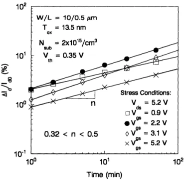
In order to accurately predict DC hot-carrier degradation, the parameters m,n,H and their bias dependencies have to be extracted precisely. The parameters m,n,H can be extracted from DC stress data. The degradation rate n can be extracted from the data shown in Figure 2.3[6]. The degradation rate n is just the slope of the line in Figure 2.3. The data in Figure 2.3 were obtained by DC stressing NMOS devices at particular bias conditions and monitoring the resulting degradation(drain current reduction) at different time intervals. The different lines in Figure 2.3 correspond to the varying stress conditions and different oxide electric field Eox. The oxide electric field is defined in terms of the gate to drain voltage Vgd=Vg-Vd, the flat-band voltage Vfb, and the gate-oxide thickness t,,ox:

V -V -V

E

g

_t

d

fb

(2.13)

ox W/L = 10/0.5 /Am T = 13.5 nm ox Nsub = 2xl1015/Cm 3 ds V = 0.35 V th

Stress Conditions:

n

V = 5.2 V

ElV = 0.9 V

SVg = 2.2 V 0.32 < n < 0.5 oV g = 3.1 V x Vg = 5.2 V gs

(21)

The EOx dependencies of the degradation rate n can be found by varying the stressing con-dition, hence EOx, and measuring the degradation rate n.

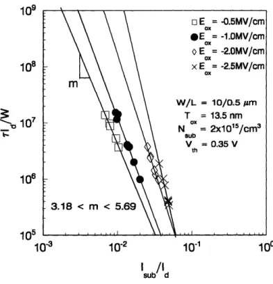
The m and H parameters can be extracted by plotting the DC device lifetime versus the current ratio l_- _{[2]. If the device lifetime definition is}_ADf,_{then the lifetime can be}

defined as follows: SAD IbjL (2.14)

f

Id

Rearranging Equation 2.14 [2]: d fn d d n sub

Equation 2.15 states that on a log-log plot of I versus , the slope will be -m

Id

and the intercept will be H.

In order to extract the parameters m and H, a set of devices has to be stressed at a

sub

series of different fixed Eox. For a given current ratio -sub,• the device lifetime r at a given

d

lifetime definition has to be calculated. The current ratio and the lifetime determine a sin-gle data point shown in Figure 2.4 [4]. The other data points on a line, which corresponds to a fixed Eox, are generated by varying Vg and Vd while keeping Eox fixed so as to change the stress current ratio. The lifetime is again calculated for the new current ratio and another point on the line is generated. The same process is repeated for the other lines in Figure 2.4 which correspond to different EOx. From Figure 2.4 and Equation 2.15 the parameter -m is the slope of the line and H is the intercept.

(22)

109 108 -- 107 106 1n5 10-3 10-2 10-1 100 sub/I d

Figure 2.4: Extracting the parameters m and H

It has been shown that the degradation parameters m,n,H have a significant oxide electric field dependency EOx[4]. Thus, it is necessary to characterize the Eox dependen-cies of the degradation parameters for predicting accurate AC degradation. The test devices used in the characterization of the EOx dependency are abrupt-junction NMOS-FETs with tox ranging from 9-19nm and Nsub ranging from lx1015 - 9x1015 and Leff > 0.4 [4]. The stress voltage (Vgd = Vg -Vd) was varied to determine the Eox dependencies of the parameters n and m.

Figure 2.5 [6] shows the degradation parameters n and m as a function of Eox. The

parameters n and m can be modeled as a quadratic function of EOx as shown in Figure 2.5. The quadratic model for the parameters n and m is as follows:

(23)

n(E = - 0.0239 x Eox - 0.0747 x E + 0.4344 (2.16)

m( E) = 0.753 x Eox + 1.144 x Eo + 3.703 (2.17)

where Eox has units of MV/cm. The degradation rate n varies significantly (0.32 < n < 0.5) over the range of stress voltages [4]. In the past, this bias dependency of n was not taken into account. The AC degradation is often predicted using either an average or peak n value. The current neff model for AC hot-carrier degradation does not model the Eox dependency accurately because it models n and m with a linear fit rather than the qua-dratic fit shown in Equation 2.16-17. Significant error can be introduced by using a linear fit for the parameters n and m, especially at low stress voltages where the Eox dependency is nearly flat. 0.5 C S0.4 0. O 0.3 E ca U) 0 50C C.) L. 0 >U) 0) 0r ,. r. 0 -0.5 -1 -1.5 -2 -2.5 -3 -3.5 -4 -4.5 -5 E (MV/cm) ox

Figure 2.5: Bias dependencies of degradation parameters m, n

9 nm < Tox < 13.5 nm

1

_

n(E ) = -0.0239*E 2 -0.0747*E + 0.4344' m(E ) = 0.753*E 2 + 1.144*E + 3.703

OX OX OX

(24)

(25)

Chapter 3 AC Hot-carrier Degradation Model

3.1 AC Hot-carrier Degradation Equations

The AC hot-carrier degradation equations are derived using the quasi-static approxi-mation. In the quasi-static approximation, the AC waveform is partitioned into small timesteps such that DC stress conditions are applicable within each timestep. Thus the degradation within each timestep can be calculated using the DC degradation model. Therefore, the AC degradation equations can be defined in terms of DC degradation equa-tions. The AC degradation equations are expressed as a set of iterative equations whereby the degradation at any timepoint is dependent on the degradation from the previous timestep

Two Step: For the two-step example, the quasi-static approximation can be used to

predict AC hot-carrier degradation. The two-step example consists of two DC stress con-ditions S₁and S₂(i.e. Vgdl (0 < t < T1) and Vgd2 (TI < t < T) over a Period=T) that

alter-nate within every cycle. The stress condition S1 corresponds to degradation rate n1 and

AGE=AGE1 and the stress condition S2 corresponds to degradation rate n2 and

AGE=AGE₂_.

The degradation (AD )until t = T1 can be calculated using Equations 2.8 and 2.12:

TI

( sub ) m

_I _mi

Id

d

t

n

,

) n

AD(TI H = (AGE 1 (3.1)

Note, that the degradation at t=T is not simply the sum of the degradation due to each of the stressing conditions:

(26)

AD (T) # AD ( T,) + f n Hd~(at 2 (A GE)I + (A GE₂) (3.2)

TI

Equation 3.2 implies that AD (T) is not a simple cumulative function of AGE when the degradation rate n varies with time. However, AD (T) can be calculated iteratively. For the two step case, AD (T) can be determined by finding an equivalent AGE=AGEeq such that the degradation resulting from this AGEeq with degradation rate n2 is equal to the

degradation after t=T1.

(AGEeq)n2 = AD( TI )= (AGE )

n l (3.3)

Solving for AGEeq:

n₁

AGEe = (AGEn2 (3.4)

Using the equivalent AGEeq notation, the n is now effectively constant (n = n2)

through-out the whole period T since now AD( T1) can be rewritten as follows:

AD(TI) = (AGEeq) (3.5)

If the degradation rate n is constant throughout the period T, the degradation at t=T is just the total age raised to the degradation rate n=n2. The total age is just the sum of

AGEeq and AGE2. Thus the degradation at t=T can be defined as follows:

n =(, 2 nn2

AD (T) = AGEeq + AGE2 2 = AGE )n2 +AGE2 (3.6)

Equation (3.6) represents the degradation at t=T using the iterative method for the two-step example. Equation 3.6 shows that the AC degradation for the two-two-step can be defined in terms of DC degradation quantities.

(27)

The same procedure is repeated when calculating the degradation at an arbitrary num-ber of cycle N. Equation 3.6 can be extended for 2 cycles using the iterative procedure:

n2 n1

AD (2T) = AGE)n2 + AGE₂ +AGEj +AGE2 ]n (3.7)

and in general the degradation for a two step waveform at t = NT is as follows:

n₁

AD(NT) = [AD((N- 1)T)] I +AGE +AGE2) (3.8)

The definition of the degradation in Equation 3.8 is recursive because the degradation at t = NT depends on the result at t = (N-1)T which in turn depends on the result t = (N-2)T and so on. Thus to calculate the degradation at the time of interest, which is usually 10

3.15x10 16

years, this will correspond to N T cycles. For a period T=10Ons, N 3.15x10 cycles, which means that Equation 3.8 is iterated 2xN=6.3x10 6 _{times since there are two}

computations per cycle for the two step example. This iterative computation can take years of CPU time which is not feasible.

General:

Equation 3.8 can be derived for an arbitrary AC waveform which is not necessarily a two-step waveform. For AC waveforms, the use of the DC quasi-static approximation limits the number of timesteps in a period of a waveform. If the waveforms are rapidly varying, then the quasi-static approximation requires that the timesteps be small. But if the waveforms are slowly varying, then the limitation on the timesteps is not as restrictive.

The degradation equation for an arbitrary waveform can be derived using arguments similar to those in Equation 3.8. The arguments used in the two-step waveforms can now be generalized for this arbitrary waveform. The degradation aftr t= At0 is just the AGE0

(28)

The degradation after t = At0 + At1 according to Equation 3.6 is:

AD( At 0 + At = (AGEO n + AGE1 (3.9)

Iterating this equation at t = At0 + At1 + At2 the degradation is:

n]

n- _{n I}

n

₂

AD( At0 +At 1 + At2 = jAGEO + AGE ni+ AGE2 (3.10)

Thus Equation 3.10 can be iterated until the desired time. Iterating further, the degradation at t=T (the degradation after one waveform cycle) can be derived:

n n_i n 2 M-1

AD (T) AGEOn +AGE) +AGE2 +...+AGEM 2 M- I+AGEM-1 (3.11)

Again, an equation can be derived for multiple cycles (i.e. N> ). n_o _n,

n₂

1 n n₂ n₃ m - 2 M

-AD(NT) (AD I (N- +AGEO +AGE + AGE ₂ + +AGEM 2 +AGEM1 (3.12)

As in the two-step waveform, calculating the degradation using the iterative Equation 3.12 is not feasible when N is large. For practical purposes, approximations have to be used to predict the degradation at t = NT with minimal error.

3.2 Two-step and AC Circuit Simulation Examples

Two-step:

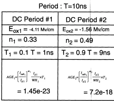
The two-step waveform example is simulated to show the degradation behavior of Equation 3.8. This equation is non-linear because within every cycle the deg-radation rate n changes as the stressing condition alternates. Sirpulated data will be shown to illustrate this non-linear behavior. For the two-step waveform there are two DC stress conditions in one period. The two DC stress conditions for the •imulations are outlined in

(29)

Figure 3.1. The degradation rate n and the voltage acceleration factor m for each stress condition are calculated using Equation 2.16 and 2.17 using the respective EOx value. The values of Eox were chosen to make the two n values (n1 and n4) differ significantly.

The parameters in Figure 3.1 were used to simulate degradation using Equation 3.8. To illustrate the non-linearity of the equation, the degradation was simulated for few cycles. The simulation result is shown below in Figure 3.2. The two lines in Figure 3.2 represent the DC degradation asymptotes determined by the AGE and n parameters within each stressing condition. The x axis is the number of cycles. Foý the simulation the period T= 10ns was subdivided into timesteps of 0. Ins such that there are 100 simulation points in one cycle and up to 1000 simulation points for 10 cycles.

From Figure 3.2, it is evident that the degradation is' linear until a tenth of a cycle(t=0. 1T) where a new stress condition is present. The degradation then flattens out

Period

:

T=10ns

DC Period #1

DC Peribd #2

Eox1

=

-4.11 Mv/cm Eox2 = -1.5i Mv/cm

nj = 0.33

n

2

= 0.46

T

1

=

0 .

1T= ns T

2

= 0.9T=9ns

r In _{___}di2 _AU/, _'d2 AGE=/- -- xT1 AGE2= ' T2 'd WH I 'I•2 WHJ

=

1.45e-23

₌

7.2e-18

Figure 3.1: DC stress conditions for the two-step waveform

when the new stress condition occurs because its contribution t the degradation is small initially. It is evident that the simulation data obeys an asympto ic behavior because it

(30)

tracks a single asymptote after only the first few cycles.

_ -7

AD(N

Figure 3.2: Degradation simulation for two-step waveform

The non-linearity of the degradation equation for the two-step example is also observed for large number of cycles. The same simulation for the two-step example was done up to N=3x107 _{cycles to illustrate this point. Figure 3.3 hows the two-step}

simula-tion data and the two DC degradasimula-tion asymptotes shown in Figure 3.2. The degradasimula-tion predicted by the current neff method is also shown. The int rsection point of the two asymptotes is labeled Nint . The simulated data in Figure 3.3 tends to track the highest

asymptote at any time. Thus the simulated data exhibits an a ymptotic behavior for the two-step example.

(31)

AD (NT)

Figure ition.

Inverter:

A similar simulation was done for an AC circ it. For this example a one-stage inverter with a capacitative load was chosen. The circuit s shown in Figure 3.4. The parameter a (V/ns) is the ramp rate of the input waveform Vi . The period of the

wave-form is T= 10ns and the width of the NMOS is Wn=40um. F r this simulation the ramp rate =10OV/ns, CL=0. lpF, and VDD=5_{v. The degradation of thý NMOS device in this}

cir-cuit was simulated for 10 cycles and the simulation result is sho n in Figure 3.5. The lines in Figure 3.5 represent the DC asymptotes.

The simulated data for the inverter in Figure 3.5 tracks one f the asymptotes just like the two-step simulation example. It also exhibits a non-linear behavior similar to that of Figure 3.2.

(32)

The non-linear behavior can also be observed for long simulations. This is shown in Figure 3.6. The simulation result show that the degradation for an inverter under AC

oper-VDD

10-1 100 10

cycles N

Figure 3.5: _{Degradation simulation for an inverter. ( W/CL} = 400pm, a = 10 V )

pF ns

(33)

~,-6

AD (NT)

10-6 10-7 10-8 10-9 10-10 100 102 104 106 1 a 010 cycles N

Figure 3.6: Degradation simulation for inverter(N=2x 108 cycles)

ating condition behaves like the DC degradation data shown ir Figure 2.3. Careful analy-sis of this simulated data will show that the degradation rate varies over time.

3.3 Current AC Hot Carrier Degradation Model(n ff)

The current neff AC hot-carrier degradation model is based on extrapolation from the first two waveform cycles. The exact degradation for the MOSFET is calculated itera-tively using Equation 3.12 for the first two cycles(i.e. N= 1,2). These two data points are used to fit the current neff model which is [2]:

neff

AD(t) = AeffX (t) (3.13)

The two fitting parameters are Aeff and neff . Since there are tw parameters, two data points are needed to solve for them.

I I I II **** Simulated Data L" nt II NE * NE * NE NE NE NE * NE NE NE NE NE NE NE NEII

(34)

The data from the first two cycles of an arbitrary waveform# can be used to solve for the fitting parameters Aeff and neff. Let AD (T) and AD (2 T) be the exact degradation from the first two cycles of an arbitrary waveform. The two fitting parameters can be solved from two equations with two unknowns as follows:

In(AD (2T) AD (7T) neff In (2) (3.14) A AD(T) (3.15) eff n eff T

The current neff model uses these two parameters in Equation, 3.14-15 to derive the deg-radation at any other time.

Two Step: For the two step waveform with the stress condition shown in Figure 3.1,

Equations 3.14 and 3.15 will reduce to the following using Eq ation 3.6-3.7:

IndI

neff = In (2) _(3.16) A AD(T) (3.17) eff neff Teff T

For the set of stressing conditions in Figure 3.1, the neff equation can be simplified to:

neff-In

In 2xAGEILn (AGE 1

In (2) n (3.18)

(35)

n2

AGE ₁ +AGE₂ (AGEI 1

Aff = nl (3.19)

eff T nl

nJ

since A GE n2>> AGE₂-. Using Equation 3.13 and 3.18-19, t e current neff model's

equa-tion can be rewritten:

AD(NT) = Aeff . W (t) _{et = NT}t (AGE 1 • (NT) ( AGE NN (3.20)

This equation is just the DC asymptote for the two-step example shown in Figure 3.3. In Figure 3.3 the DC asymptote, represented by Equation 3.20, u derestimates the degrada-tion for N > Nint. Thus the current neff method underestimated the degradation for the

two-step example. The error introduced by the extrapolation cln be significant if the inter-section point Nint occurs very early in time.

Inverter: The main problem with the current neff model is the possible error that can

result by extrapolating from just the first two cycles to 10 y ars(-1016cycles) which is usually the time point of interest. The extrapolation error may seem small since the AC degradation appears to be linear in Figure 3.6 for the case ofl an inverter. However, this assumption is not correct because if a line was used to fit the simulated data in Figure 3.6, the slope of the line will change as more and more data points are used for the fitting.

To illustrate this point, a line was used to fit different numbers of data points from Fig-ure 3.6. For each fit the slope of the line, n, was calculated to ýhow that the AC degrada-tion is non-linear. If the slope of the line did not change as more data points were used for the fitting, this would imply that the degradation was linear and that the degradation rate n was constant. However, for the inverter degradation in Figure 3. , the slope of the line

(36)

var-ies as more data points are used to do the fitting. This implvar-ies that the AC degradation for the inverter is non-linear. The result of the fit is shown in Figtore 3.7 where the x axis is the number of data points used in the fit and the y axis is the sl pe of the line that fits these data. As more data points are used to fit the line, the slope of ýhe line(n) increases.

0.46 .

0.4006

-0.38

-g-0.449

10' 1data points

Figure 3.7: Degradation rate n as a function

of number of data points used for fitting.

Thus by using only the data from the first two cycles(current neff method), the varia-tions in the degradation rate n are not taken into account. The hange in n is about -0.05 according to Figure 3.7 for N=2x108 _{cycles but after 1016 cycles (-10 years) this change}

can become significant. Since the overall AC degradation is a sensitive function of n, small changes in n can have significant effect on the degradati n. The degradation rate is dynamic and can have an appreciable change over many cycles and cannot be modeled accurately using only the first two cycles. Therefore different degradation rate n's are needed to model degradation accurately depending on the time f interest.

lI lI lIE lIE IN lIE INm IN IN INm INm *m INm

(37)

Fast Transients: In special cases where the transition ioi the voltage waveforms(Vg

and Vd) is very fast, the current neff method can actually p edict the degradation accu-rately. Sharp transitions in the voltage waveforms will result in an impulse-like substrate current. A ring oscillator is a good example of a circuit where the substrate current exhib-its such an impulse-like waveform. If the substrate current ýs impulse-like, the variable A(t) defined in Equation 2.9 will also be impulse-like. Equation 3.12 will reduce to an equation with only a single dominant degradation rate n. If tIe impulse occurs at the kth time interval in a period T, then the exact degradation at any t me is approximately:

AD (NT) (AGEk x n k (3.21)

Solving for neff and Aeff using Equation 3.14 and 3.15:

(AD(2T) nx In AGE n In 7 k AGEk eff In (2) In (2) = (3.22) n AGE k AGE)nk A eff = Tk(3.23) eff T AGE nk nk nk

AD (NT) = Aeff (NT) eff - (NT) = (GE k xN (3.24)

Thus for impulse-like waveforms the current neff method can accurately model the degra-dation because only one n dominates. But for most circuits the substrate current waveform cannot be approximated as an impulse so that the current nff niethod has limited aoolica-tion.

(38)

(39)

Chapter 4 New Model for AC Hot-carrier Degradation

4.1 Concept of Dominant Asymptote

The AC degradation for both the two-step and the inverter example examined in Chap-ter 3 exhibited asymptotic behavior. It has been shown that tle current neff method's life-time predictions tend to diverge away from the true solution while an appropriately chosen asymptotic solution approaches the true solution. Therefore, the new model for AC hot-carrier degradation is based on the concept of a dominant asymptote. The new model's algorithm identifies the asymptote that accurately defines the C degradation behavior of a device due to hot-carrier injection at the future time point of interest.

4.2 Formulation of the Initial Degradation Asymptote

An asymptote can be defined by two parameters AGE and as follows:

AD(NT) = (AGExN)n (4.1)

The first step in the algorithm for the new model is to generate an initial asymptote as a guess about the degradation at the time point of interest. The irst asymptote is generated by calculating AGET and n for the particular AC waveform. Assuming the AC waveform has a period T, then the variable AGET, the total AGE in a period, is defined as follows using Equation 2.8:

T

AGET = AGE(T) = • dt (4.2)

0

where the integrand is a function of time. The integration above is done numerically using the trapezoidal approximation shown in Figure 2.2.

(40)

Next, in Figure 2.2, an AGE=AGEi and degradation rate =ni can be defined at the ith

timestep, where i ranges from 0 to M- 1, for each of the sub-i tervals within the AC wave-form. The degradation rate n=n of the initial asymptote is t en defined as the average of all the ni's in a waveform period weighted by their respectivi AGEi's. Thus, the average

n=n is defined as follows:

M-I

Sni

"AGE

_i

n 0A-AG-ET (4.3)

where AGET in the denominator is defined in Equation 4.4 us ng Equation 2.11:

M-1

AGET = _AGEi (4.4)

0

This completes the specification for the initial asymptote. The jequation of the initial asymptote is defined below:

AD (NT) = (AGET x N) (4.5)

Equation 4.5 will be used as a trial guess for the degradation a1 the time-point of interest.

4.3 Partitioning of the Asymptotes

The second step in the algorithm is to generate two asymptotes from the initial asymp-tote by partitioning the initial asympasymp-tote. The partitioning sch me involves several steps. For the illustration of these steps, an inverter example lis used(w/cL = 40 p ,

a = (•). The first of these steps is to generate a plot of n v rsus time for the period of the waveform. This is shown in Figure 4.1. In Figure 4.1, give 1 n as a function of Eox, n can be calculated at every timestep using the value of Vgd (and Ilence Eox) at that timestep.

The second step is to plot the instantaneous AGE in each tim shown in Figure 4.2. The next plot, shown in Figure 4.3, is to pl(

estep versus time. This is

(41)

0.2 0.3 0.4 0.5

time

Figure 4.2: Instantaneous AGE

(42)

Figure 4.3: Cumulative AGE versus

time. Cumulative AGE at some time to is defined to be the are under the curve in Figure

4.2 until time=to.

The degradation rate n versus cumulative AGE is shown in igures 4.4 and 4.5. The x-axis is the cumulative AGE at some time t and the y-x-axis is t le degradation rate n at the same time t. The horizontal lines shown in Figures 4.4 and 4.5 correspond to the average n. The line labeled n is calculated using Equation 4.3.

This line defined by n is then used to partition the initial a ymptote into two compo-nents. The two components are defined by the parameters AGE , n1, AGE2, and n2 shown

(43)

in Figures 4.4 and 4.5. The total AGET is the sum of rates n1and n2 are the average of the n's weighted by

AGE1 and AGE2. The degradation

AGE b low and above the

10-24 10-22i

AGE

Figure 4.4: n versus cumulative AGE(semi og plot)

n=n respectively. The equations for nl and n2 are defined below:

10-20 I ni " (AGEi) 0 < AGE < AGE AGE i ni- (AGEi)

AGE_I<AGE < AGE7

AGE₂

The equations that describes the two asymptotes generated are:

from the initial asymptote

n

0.4E 0.44 0.42

0.4

0 Qp n

12 AGE

1 AGET=AG

_E+AGE

₂

CE!

10-26 partitioning line (4.6) (4.7) r n2 ₂ =

(44)

ADI(N7) =(AGEl XNN)l AD2(NT) = (AGE2 xN)n 2 0.5

n

0.48 0.46 0.44 0.42 0.4 0.38 0.36 0.34 0.32 0.3 00 0.2 0.4 0.6 0.8 (4.8) (4.9) 1

AGI

Figure

4.5:

n versus cumulative AGE(line scale)

Figure 4.4 is plotted again in Figure 4.5 with a linear scale.

EJ x 10-0

4.4 Identifying the Dominant Asymptote

The next step in the algorithm is to identify the dominant asymptote at the time of interest. The dominant asymptote indicates the highest degradation at the time point of interest. Figure 4.6 illustrates the procedure of identifying the

time of interest (N=Nsp). The initial asymptote is partitioned i in the previous section to generate two asymptotes A1and A2.

asymptote at the nethod described mptotes, the

orig-1

n

-i

AGE

1 AG

(45)

inal and the two i asymptote A1 doi

Next, each o procedure for the has been reached

Figure 4.6, g the same legradation and A₂₂. nterest mptote A1

A

A₂ Nsi N(cycles)

Figure 4.6: Identifying the dominant asymptote

After each partitioning, the algorithm compares all the asymptqtes and identifies the dom-inant asymptote at the time of interest. The process of partitioning each of the generated asymptotes and noting the dominant asymptote is repeated untii the partitioning results in

one of the AGE quantities being very small:

AGE1 << AGE2 (4.10)

(46)

AGE2 << AGEI1 (4.11)

The tolerance used for the AGE quantities was if any one bf the AGE<1x 10-50 _{then the}

partitioning stopped. When the partitioning of all the asympt tes stopped, then the degra-dation at the time point of interest is defined by the most dominant asymptote that has been identified. The notation used for the dominant asymptote is n=ndom and

AGE=AGE-domD The degradation at the time point of interest(N=Nsp) is then

ADI(NWT) = (AGEdo,mXN) dom

For calculating the lifetime of the device, the same steps lsed for degradation calcula-tion are followed except that the goal of the algorithm for lifetime calculacalcula-tion is to find the asymptote that will minimize the lifetime(at the given lifetime definition AD ). Thus, for

_f

each asymptote, the lifetime will be calculated inste

4.12. The asymptote with the minimum lifetime will

AD (NT)

I I

using Equation e of that device.

L2 Li 1 Cycles

Figure 4.7: Lifetime calculation using dominani

L

i

I

i

i i w

(47)

In Figure 4.7 the initial asymptote and two asymptotes(A and A2) generated by

parti-tioning the initial asymptotes are shown. The lifetime of the device is calculated by find-ing the asymptote with the minimum lifetime usfind-ing the same lgorithm for the calculation

(ADf) .T

AE = (4.12)

AGE

of degradation. From Figure 4.7, asymptote A2 predicts the smdallest lifetime(L2<Li<L1) at

the lifetime definition ADf. If the asymptotes in Figure 4.7 r present all the possible

asymptotes that can result from partitioning the initial asympt te then the lifetime is defined by asymptote A2. The lifetime defined by asymptote 42 is the closest to the exact

lifetime defined by the dashed line which represents the exact Oegradation. In general, the asymptotes may have to be split many times before the minimpm lifetime is found.

4.5 Two-step and Inverter Examples

Two-step: The two-step example can be used to illustrate why the dominant

asymp-tote method is a more accurate method for predicting the AC Iegradation of a MOSFET. There are two domains of interest for the two-step example where two different degrada-tion components dominate depending on the time of interest. In Figure 4.8, the simulated degradation for the two step waveform using the stress conditicns outlined in Figure 3.1 is shown along with the current neff method. In addition, the do inant asymptotes defined using the new method are shown in comparison. The equati ns that describes the two dominant asymptotes are as follows:

for N < 105cycles:

(48)

for N > 105cycles:

AD(NT) = 7.2x10- x18xN) (4.14)

Using the current neff method, the equation for the line as shown in Figure 4.8 from Equa-tion 3.18-19:

n

AG~n 1n

n)I

AD(NT) = Aeff (NT) n•AGE (NT) AGE I N) (4.15)

-23 0.337

- (1.45 x 10- 2 3 N) 0.337 (4.16)

Thus for N<105 cycles, the current neff and the new meth d predict roughly the same amount of degradation. But for N>105 cycles, the new method models the AC degradation closer to the exact simulation data as shown in Figure 4.8, w#ile the current neff method deviates gradually away from the exact data. This is becaus the dominant degradation rate n

AD ( NT)

(49)

hc anges after N>105 cycles. The 05

cycles and thus Equation 4.14 using the new method predicts rately.

Inverter: An inverter example shown in Figure 3.4 is a new algorithm. For this example CL= lpF and at = 5 V/ns. I generated by the partitioning method are shown for the typic

the degradation more

accu-Iso used to demonstrate the Figure 4.9, the asymptotes al inverter simulation along with the simulated data. The initial asymptote in Figure 4.9 is labeled accordingly and the other asymptotes generated from splitting the initial asymptot• and other resulting asymp-totes are shown. T1

where 10-6 AD (NT) 10-7 10- e 10-9 10- 10 10- 11 1

Figure 4.9: Demonstration of the algorithm for Ian inverter

the process of splitting the asymptotes results in the identificati n of a dominant asymp-tote. The AC degradation at 105_{cycles is determined by this do ninant asymptote.}

(50)

For this example, table 4.1 shows the numerical result o the asymptote splitting and the degradation at 105 cycles. The first column lists the nota ion used for the asymptotes. The second two columns of the table represents the AGE a d n respectively that define each of the asymptotes shown in Figure 4.9. The last column on the table is the degrada-tion value predicted by the asymptote at 105 cycles. The de radadegrada-tion values in table 4.1 fluctuate with each new asymptotes and eventually one of the asymptotes predicts the maximum degradation. The maximum degradation is shown

Table 4.1: Numerical results for NMOS in invertl

Asymptote _AGE

n

Notation AD (NT)

A0, no 7.7680e-21 4.7702e-01

6.199766e-Al_,nl 3.2480e-21 4.9202e-01 2.395550e-A2, n2 4.5199e-21 4.6623e-01

7.010689e-A21, n2 1 4.0187e-21 4.7075e-01

5.654227e-A2 2, n22 5.0122e-22 4.3003e-01

9.784152e-A -- A '2 "- 1 1 A A'I.III f'•l l IC• •" AAA" A

ith an asterisk.

r at N=10s cycles

A22 1, n221 4.z239e-22 4.4LL2e-U1 5.7•5-444e-U1

A2 22, n222 7.7264e-23 3.6324e-01 6.084555e-67***

The first line in table 4.1 represents the initial asymptote. Ior this example, the initial maximum degradation is - 6.2e-8. After the first split, the maximum degradation is changed to -7e-8. The maximum degradation increases to -9.+e-8 in the second split and to -6.1e-7 in the last split. The asymptote labeled "dominant asymptote" represents the maximum degradation after the three splits. The degradation at 105 cycles is -6.1e-7 according to the new algorithm. This result agrees well with th simulated degradation at 105 cycles which is approximately 6.11 e-7.

48 = (AGE x N) n 38 )8 )8 )8 08 4)

(51)

4.6 Implementation of the New Model using a C l rogram

This section describes the detail of how the algorithm cemonstrated in the previous section can be implemented using the C programming langu4 ge. The program that imple-ments the algorithm is essentially a post-processor, which moeans that it executes the code using results from another program. The program code is listeWd in appendix A. In this case the results that the program needs is the output from SPICE and the output from BERT(BErkeley Reliability Tools). In addition it requires the nodel parameters for m,n,H degradation parameters and other information relevant to the eircuit under test.

The first input to the program is the output of SPICE. Thi_Ioutput from SPICE has the data for the voltage waveform(Vg, Vd), and drain current I_d.The SPICE input netlist

con-tains commands to print out the Vg, Vd and Id value at each timestep for each NMOS device in the circuit. The voltage waveforms (Vg, Vd) are eeded to calculate the Vgd (hence Eox) bias dependencies of the degradation parameters in,n,H as described in chap-ter 2. The drain current Id is used to calculate the variable AGE defined in Equation 2.8.

The drain current in SPICE is calculated using the BSIM level 13 SPICE model.

The other inputs to the program is the substrate current o tput from BERT. BERT is used to calculate the substrate current using the substrate curre it model described in chap-ter 2. BERT calculates the substrate current at the timestep dechap-termined by the SPICE sim-ulation[5]. The substrate current data is used to calculate the A3E variable.

Other inputs to the program include the SPICE input netlist file, which has information pertaining to the circuit, and other user inputs. These information include the device width W, which is necessary to calculate AGE and the period T which is necessary for calculat-ing the lifetime of the devices. The user input includes the specifcation of the lifetime def-inition, user snecified time noint(for calculation of degradatinn) aind the model narameters

(52)

The role of the program is to take all these inputs and prccess it to produce the output which is the degradation and lifetime of each devices at the tser specified time point and lifetime definition respectively. The overall structure of the program is shown in Figure 4.10 with the inputs and output for the program.

In stage 1 of Figure 4.10, the output of SPICE and BERT for the NMOS devices are processed so that they can be readable by the program. Tho device width, W, and the period of the waveform T can be obtained from the SPICE n tlist which is another input.

m mn Tmnrdel

W,

T

Vgd

'sub

Stage 2 Stage 3

Figure 4.10: Structure of the new mocel

The degradation parameters along with their bias dependency 4re also the inputs to the second stage of the program. These inputs suffice to do the caldulations for AGE and n which are necessary for formulating the degradation asymptote

In stage 2, the processed information can be used to imp emnent the new model. At each timestep of the SPICE waveform, the program calculates rgd=Vg-Vd in order to

cal-Dominant Asymptote Algorithm Degradation at user specified time Lifetime at user specified definition I - • liuuLl I I - A I I i I - I I I I

(53)

culate Eox. Then it calculates the degradation parameters n,n,H as a function of the bias Vgd at this timestep. The next step is to calculate the variable AGE=f(Id, Isub, W,m,H). To

calculate AGE, which is the integral of the waveform shown in Figure 2.2, the substrate current Isub and drain current Id are read from the output of the SPICE and BERT simula-tion at each timestep. The AGE in each timestep is calculated by using the trapezoidal method. The process of computing n and AGE is done for pach timestep in the SPICE analysis and the result is stored in data files.

These data are then used to calculate the initial asymptote The partitioning of the ini-tial asymptote is accomplished by a function that takes arrays of data with all the n's and AGE at each timestep and creates two sets of arrays by partitioning the n's and the AGE with n=n .These arrays can be used to determine the two asymptotes generated from the initial asymptote. The partitioning is continued until the asym totes cannot be partitioned further. The maximum degradation and the lifetime are event ally determined and stored in a file specified by the user in stage 3. For multiple devices in a circuit, the same proce-dure is repeated and the results for each transistor are stored in one user specified file.

(54)