HAL Id: hal-02262908
https://hal.inria.fr/hal-02262908
Submitted on 2 Aug 2019HAL is a multi-disciplinary open access archive for the deposit and dissemination of sci-entific research documents, whether they are pub-lished or not. The documents may come from teaching and research institutions in France or abroad, or from public or private research centers.
L’archive ouverte pluridisciplinaire HAL, est destinée au dépôt et à la diffusion de documents scientifiques de niveau recherche, publiés ou non, émanant des établissements d’enseignement et de recherche français ou étrangers, des laboratoires publics ou privés.
Distributed under a Creative Commons Attribution| 4.0 International License
MuSCA: a multi-scale source-sink carbon allocation
model to 2 explore carbon allocation in plants. An
application on static apple-tree
Francesco Reyes, Benoit Pallas, Christophe Pradal, Federico Vaggi, D
Zanotelli, Tagliavini Marco, D. Gianelle, Evelyne Costes
To cite this version:
Francesco Reyes, Benoit Pallas, Christophe Pradal, Federico Vaggi, D Zanotelli, et al.. MuSCA: a multi-scale source-sink carbon allocation model to 2 explore carbon allocation in plants. An application on static apple-tree. Annals of Botany, Oxford University Press (OUP), 2019, �10.1093/aob/mcz122�. �hal-02262908�
1
Original Article 1
MuSCA: a multi-scale source-sink carbon allocation model to
2
explore carbon allocation in plants. An application on static apple-tree
3
structures.
4
F. Reyes1,2,3,*, B. Pallas4, C. Pradal4,5, F. Vaggi6, D. Zanotelli3, M. Tagliavini3, D. Gianelle2, E. 5
Costes4 6
1
DAFNE, 01100 University of Tuscia, Viterbo, Italy, 2DASB, CRI, Fondazione E. Mach, 38010 San Michele
7
all'Adige, Italy, 3Faculty of Science and Technology, Free University of Bozen-Bolzano, 39100 Bolzano, Italy, 4AGAP,
8
Univ. Montpellier, CIRAD, INRA, SupAgro, Montpellier, France, 5CIRAD, UMR AGAP & Inria Zenith, Montpellier,
9
France, 6Amazon, 98100 Seattle, USA, 7INRA, UMR 547 PIAF, F-63000 Clermont-Ferrand, France
10
Running title: MuSCA multi-scale carbon allocation model
11
*
For correspondence. Email [email protected]
12 13
2
ABSTRACT
1
Background and aims
2
Carbon allocation in plants is usually represented at a topological scale, specific to each model. 3
This makes the results obtained by different models, and the impact of their scales of 4
representation, difficult to compare. In this study, we developed a Multi Scale Carbon 5
Allocation model (MuSCA) that allows using different, user-defined, topological scales 6
of a plant, and assessing the impact of each spatial scale on simulated results and 7
computation time. 8
Methods
9
Model multi-scale consistency and behavior were tested on three realistic apple tree structures. 10
Carbon allocation was computed at five scales, spanning from the metamer (the finest 11
scale, used as a reference) up to 1st order branches, and for different values of a sap 12
friction coefficient. Fruit dry mass increments were compared across spatial scales and 13
with field data. 14
Key Results
15
The model was able to represent effects of competition for carbon assimilates on fruit growth. 16
Intermediate friction parameter values provided results that best fitted field data. Fruit 17
growth simulated at the metamer scale differed from about 1% at growth unit scale up 18
to 60% at first order branch and fruiting unit scales. Generally, the coarser the spatial 19
scale the more predicted fruit growth diverged from the reference. Coherence in fruit 20
growth across scales was also differentially impacted, depending on the tree structure 21
considered. Decreasing the topological resolution reduced computation time by up to 22
four orders of magnitude. 23
Conclusions
24
MuSCA revealed that the topological scale has a major influence on the simulation of carbon 25
allocation. This suggests that the scale should be a factor which is carefully evaluated 26
when using a carbon allocation model, or when comparing results produced by different 27
models. Finally, with MuSCA, trades-off between computation time and prediction 28
accuracy can be evaluated by changing topological scales. 29
Keywords: MuSCA, multi scale, carbon allocation, plant growth, tree growth, functional-structural
30
plant modeling, FSPM, multiscale tree graph, source, sink, apple, plant architecture 31
3
INTRODUCTION
1
Carbon allocation is the process by which carbon assimilated by leaves, or stored in the form 2
of carbohydrates, is transferred, via the conductive vessels (or phloem tissue) to other plant parts, 3
where it is used primarily for respiration and growth. It is generally accepted that the phloem sap 4
moves as a consequence of osmotically generated pressure gradient, as described by the Munch 5
theory (Münch 1930). Gradients are generated by the differences in the concentrations of carbon 6
(C) assimilates between C-sources (mainly leaves, where C-assimilates are loaded into the phloem) 7
and sinks (where C-assimilates are unloaded from the phloem). The Münch theory has been refined 8
over time (e.g. with the introduction of the leakage-retrieval mechanism (Thorpe et al. 2005) and 9
complementary hypotheses have been proposed to explain the lack of fit with experimental 10
evidences (e.g. sieve tubes decomposed in shorter, overlapping components, at the edge of which 11
solutes are transported at the expense of internal energy) (De Schepper et al. 2013). The underlying 12
principles, however, are still considered as valid. As such, the C-allocation process is thought to 13
depend primarily on the amount and distribution of the available C-supplies, on demands along the 14
plant structure and on the possibility of C-supplies to flow via the phloem (Ryan and Asao 2014). In 15
models of small plants, however, the simplifying assumption that distance has no effect on C-16
availability or phloem osmotic potential (known as the ‘common assimilate pool’) can be made 17
(Heuvelink 1995; Guo et al. 2006; Luquet et al. 2006; De Swaef et al. 2003). 18
When plant topology increases in complexity, the modeling approaches to C-allocation 19
present in the literature can be organized in four, partly overlapping, categories (Thornley and 20
Johnson 1990; Lacointe 2000; Le Roux et al. 2001; Génard et al. 2008): models based on empirical 21
relationships between plant parts and/or the environment; teleonomic models representing the plant 22
as moving towards an a priori defined specific state; source–sink driven models, in which different 23
plant components are supposed to attract C-assimilates with different strengths and lastly transport 24
resistance and biochemical models, which represent phloem transport as starting from osmotic 25
gradients and biochemical conversions. The most mechanistic models, which represent osmotic 26
flows as starting from osmotic gradients, imply complex formalizations and highly detailed plant 27
descriptions and therefore received relatively limited attention (Bancal 2002). The modest 28
mathematical complexity of source sink models has led to them becoming the focus of a much 29
larger number of studies. In all cases the representation of C-allocation on large tree structures 30
described at high resolution remains computationally intractable (Balandier et al. 2000; Bancal 31
2002). 32
Each model represents the plant structures, and the process of carbon allocation, at a specific 33
scale. The choice of scale may be driven by management or research needs, by the computation 34
4
time needed for the simulations and by the resolution at which the calibration and testing data was 1
obtained. Such scales range from the individual metamer (M) (Allen et al. 2005) to collections of 2
metamers that, grouped according to criteria such as their age, position or organ type (Kang et al. 3
2008), constitute larger portions of a tree structure, such as branches, main axis or even whole plant 4
compartments (Lakso and Johnson 1990; Kang et al. 2008). 5
By way of example, the L-PEACH model (Grossman and DeJong 1994; Allen et al. 2005) is 6
a reference for completeness of the described processes and represents tree growth over multiple 7
years. This uses a transport resistance analogy to mimic C-transport at the M scale (internode, leaf, 8
fruit). The SIMWAL model represents the growth of a young walnut tree across several years. This 9
is organized in axes, which are divided into growth units (GU, the scale of C-allocation), 10
themselves composed of internodes and nodes (Balandier et al. 2000). A GU is an organisation 11
level typical of plants with rhythmic growth. It corresponds to a portion of axis developed without 12
interruption during an elongation period, and can be visually identified as bounded by two zones of 13
scales that had protected the apical meristem in the bud during resting period. The QualiTree model 14
represents growth and quality of fruits on a peach tree structure, at the fruiting unit (FU) scale, 15
during a single growth season (Lescourret et al. 2011, Pallas et al. 2016). A FU includes the set of 16
shoots born from a common section of one year old wood. In this model all the different types of 17
organs in a FU are considered similar with respect to assimilates exchange, which depends on their 18
respective distances only. 19
The computation of C-allocation by a model is affected by both the formalism used to 20
describe the physiological processes and the discretization of the plant. Because of this, identifying 21
what causes differences in results produced by different models can be difficult. 22
The present work proposes a new, source-sink, Multi-Scale Carbon Allocation model 23
(named MuSCA), whose aim is to allow for a flexible definition of topological plant scales 24
concomitant with the simulation of carbon allocation. The model relies on the use of Multi-scale 25
Tree Graph (MTG) (Godin and Caraglio 1998), a formalism inspired by the observation of the 26
multi-scale organization of plant structures (Barthélémy 1991; Barthélémy and Caraglio 2007; 27
Balduzzi et al. 2017). MTG allows for the topological description of a plant at multiple, nested, 28
spatial scales on the same graph. In addition to the connections and boundaries of the described 29
topological scales, intensive (e.g. organ type) or extensive (e.g. geometrical features) properties can 30
be assigned to the individual plant component at any scale. MTG has been previously used in plant 31
architecture analyses (Costes et al. 2003), in radiation interception (Da Silva, Han, and Costes 32
2014), as well as to simulate physiological processes (Fournier et al. 2010; Ndour et al. 2017; 33
5
Barillot et al. 2018) or model plant-pathosystems (Garin et al. 2014, 2018; Robert et al. 2018) 1
(albeit by using a single scale at a time). 2
In this paper, we provide an overview of the MuSCA model, define its scope and inputs, 3
present the formalisms used to compute C-allocation and to move across scales. The model is 4
calibrated for the apple tree (Malus x domestica Borkh.), Fuji cultivar, for C-demands. It is linked to 5
a radiative model for the estimation of C-assimilates by leaves. The model is then applied on three 6
contrasted apple tree structures and for different values of an empirical sap friction parameter, and 7
the effects of competition for C-assimilates on fruit growth are analyzed. Field observations are 8
then compared to the fruit growth distribution simulated on one tree structure to retain the sap 9
friction parameter values that might best represent sap flow dynamics. The ability of the multi-scale 10
formalism to produce similar results across scales and the influence of the scale of representation on 11
the simulated carbon allocation are analysed. Finally, the trade-off between computational 12
efficiency and accuracy are discussed, also in respect to the possible interactions between specific 13
tree structure and the topological scale used. 14
MATERIALS AND METHODS
15Model Description
16Overview
17
MuSCA is a generic, functional structural plant model (FSPM) (Vos et al. 2010) 18
representing the carbon allocation and organ growth of a plant at different, user-defined, spatial 19
scales, while taking into account competition and distances between carbon sinks and supplies 20
present on the plant (Fig.1). The model has a modular architecture and each module is generalized 21
so that only a few of them are specific to a given cultivar or species (Table 1, Table 2). The model 22
is integrated in the open-source OpenAlea environment (Pradal et al. 2008, 2015) and implemented 23
in the Python language. The model reuses existing OpenAlea components, such as the MTG 24
dynamic data-structure (Godin and Caraglio 1998; https://github.com/openalea/mtg), used to 25
represent the multiscale topology of plant structures, the PlantGL library (Pradal et al. 2009) used to 26
represent the 3D geometry, and the RATP radiative model (Sinoquet et al. 2001). The MuSCA 27
model simulates biomass accumulation over a single vegetative season. 28
Input plant structures and creation of new scales
6
The input plant structures of MuSCA are MTGs where individual plant components are 1
characterized by qualitative or quantitative information. Qualitative information refers to the organ 2
type or the type of connection between vertex and parent (i.e. branching or succession). 3
Quantitative information may include parameters such as the geometry or age of a plant component. 4
This information can be used to create criteria defining the membership of individual plant 5
components to larger groups of adjacent plant components. 6
Movement of carbon
7
The movement of the available carbon (Fij), from a C-supply (i) to a C-sink (j), is 8
represented as a function of the C-available in the supply (ACPi), the sink C-demand (Demandj) (eq. 9
1a), and is inversely related to the distance (dist) between source and sink and to a sap friction 10
parameter (h) (eq. 1b), along the plant topology. The h factor is an empirical friction parameter, 11
proposed in previous source-sink carbon allocation models (Balandier et al. 2000; Lescourret et al. 12
2011). Larger values of this parameter amplify the effects of distance resulting in relatively large 13
amounts of C allocated next to the source, while a value of zero implies no effect of distance. This 14
equation is inspired by a previously defined equation (SIMWAL model, Balandier et al. 2000). 15 16 = ∗ ,ℎ ∗� � ∑�=1 ∗ ,ℎ (eq. 1a) 17 � , ℎ = + ℎ (eq. 1b) 18 19
If in excess, the C-allocated to a plant component will just fulfill its C-demand, while the 20
excess will be stored in a reserve pool for this compartment and be considered as a supply provided 21
by that component on the following time-step (Balandier et al. 2000). However, since simulations 22
in this study lasted for only one day, this phenomena never occurred. 23
The carbon allocated to a topological element is eventually divided among the different 24
organs that constitute it (at the metamer scale: fruit, leaf, internode), proportionally to their 25
individual carbon demand. 26
Calculation of distances
27
A representation of the C-allocation process coherent at multiple topological scales requires 28
the definition of an equation for the calculation of distances, independent of the scale of 29
representation. 30
7
Modeling C-allocation is computationally demanding as, in a source-sink formulation, it 1
requires to compute the distance between all pairs of carbon sinks and sources in the tree. In a 2
MTG, sources and sinks are represented by vertices in a tree graph. The complexity of computing 3
the distance between all pairs is quadratic, i.e. requires around n2 operations, for a tree of n 4
vertices. We thus designed an algorithm, based on the multi-scale organization of plants, which 5
allows to reduce the number of operations by reducing the number of independent plant vertices 6
that must be compared. 7
Each MTG vertex (i) is characterized, among other properties, by three dimensional 8
coordinates (basal and top), the possibility to have a parent (named i-1), and one or multiple sons 9
(the vertex i is the son of its parent). In a MTG, a vertex at a coarser scale (I, called complex) is 10
composed of one or more vertices at the finer scale (called components of I), as in the case of a 11
shoot composed of several internodes. 12
The distance (disti,j) among two vertices (i, j) in a MTG depends on the sequence of vertices 13
that connect i and j (called topological path). It corresponds to the sum of i) the semi-lengths of the 14
extremities i and j, and ii) the length of the topological path between the bases of i and j (eq. 2a, 2b 15
Fig.2). The semi-length of an element at different scales is computed as the distance between its 16
base and barycenter. 17
In order to assess the length of this path, it is necessary to identify the Greatest Common 18
Ancestor (GCA) of vertices i and j (Fig.2). Given the two paths connecting the tree root to i and j, 19
the Greatest Common Ancestor of vertex i and vertex j, GCA(i,j), is identified as the vertex that is 20
contained in both paths and that is the closest to i and j. The topological path between i and j is the 21
union of the vertices between i and GCA(i,j) and the path between j and GCA(i,j) with GCA(i,j) 22
(Fig.2). The length of the path (disti,j) is computed as the sum of the length of each of its internal 23
elements plus the semi-lengths of its extremities, minus twice the length of the GCA (Fig.2, eq.2a). 24
In addition, the distance between the basis of the first two elements of the path, that are directly 25
inserted in the GCA(i,j) and are not connected with each other, is added (eq.2a). This is the case at 26
corser scale when different ramifications are connected to the trunk at different location. When the 27
GCA is either i or j, the length is just the sum of the length of all its internal elements plus the semi-28
length of its extremities (eq.2b). 29 30 � , = � � ��� ℎ + � ,� �+ � ,� �+ � � ��� ℎ − 2 ��� ℎ � + 31 � � �� , � �� (eq. 2a) 32 33
where � � �(resp. j) is the first descendant in the path(i,GCA(i,j)) (resp. j). 34
8 1 if GCA is i or j, 2 � , = � − , − + � � ��� ℎ + � � ��� ℎ (eq. 2b) 3 4
The calculation of the spatial coordinates of the basis and barycenters depends on the scale 5
(Fig.2B). At M scale, the basal coordinates of a vertex correspond to the top coordinates of its 6
parent vertex (eq. 3a). For the basal vertex of the MTG, the only without a parent, coordinates are
7
stored in the complex of the same vertex. Barycenter coordinates are obtained as the mean of its top 8
and base coordinates (eq. 3b). 9
At coarser scales, the basal coordinates of a vertex I are the basal coordinates of its first 10
component at the metamer scale i.e. the one whose parent does not belong to I (eq. 3c). These basal 11
coordinates are inherited from top coordinates of its parent (see eq. 3a). 12
Regarding the coordinates of the barycentre of a coarse scale vertex, these are calculated as 13
the mean of the coordinates of the barycenters of its components, weighted by their individual 14
lengths (as in eq. 3d for the x coordinate). 15 16 At metamer scale: 17 � = (eq. 3a) 18 � �� � �, = �,+ � (eq. 3b) 19 At coarse scales: 20 ∀ i ⊆ I | parent(i) not ⊆ I: 21 �� = (eq. 3c) 22 23 � �� � �,� =∑ � �,∗ ℎ ∑ ℎ (eq. 3d) 24 25
Up- and down- scaling
26
In MuSCA, some of the plant properties available at one scale are used to provide a 27
description of the same properties at a coarser (up-scaling) or finer (down-scaling) scale. This is 28
done in simulations running at coarse scales, prior and after the calculation of carbon flows, 29
respectively by calling up- and down- scaling functions (except for the initial calculation of 30
biomasses, see part From geometry to biomass). The up-scaling of properties such as biomass, 31
carbon supplies and demands of plant parts is simply done by summing up the property values 32
9
stored in all the vertices that are contained within the topological boundaries of the coarser scale 1
component. Conversely, down-scaling the same properties from a coarse scale component to its 2
constituting elements requires some assumptions. In particular, when the carbon allocated to a 3
coarse scale component is down-scaled, it is assigned proportionally to the relative carbon demands 4
of its constituent elements. 5
Application to realistic tree structures: the case of apple (Malus x domestica Borkh)
6In order to assess the ability of the model to simulate similar growths across multiple scales, to 7
represent competition for C-assimilates and the effect of the scale on computation time, we applied 8
MuSCA on different tree structures of apple trees, represented at multiple topological scales). These 9
were MTGs of three apple trees simulated by the MAppleT architectural model (Costes et al. 2008). 10
MAppleT combines markovian models for the simulation of growth unit succession and branching 11
with a biomechanical model for axis bending. Along growth units, individual leaf area was 12
simulated based on a logistic function and assuming different final values of leaf areas for the 13
preformed (7 leaves) and neoformed parts of the GU (Da Silva et al., 2014a). This model was 14
previously calibrated on Fuji cultivar (Costes et al., 2008) and so that it could be used to generate 15
one four year old ‘Fuji’ tree that was used in this study. Moreover, two other trees were simulated 16
by initiating simulations using two different sequences of lateral types along the trunk observed on 17
trees originated from a bi-parental population, as previously proposed by Da Silva et al. (2014b). 18
These two trees were selected within the population in order to test our C allocation model on trees 19
displaying contrasted architectures. Simulations were run for each individual tree on a single day, so 20
that the direct effect of changing the topological scale could be analyzed while excluding possible 21
retroactions and cumulative effects (such as the re-use of C delivered in excess to a plant 22
component). A partly cloudy day of late June (day of the year = 182) was chosen to drive 23
photosynthesis. This allowed on the one hand C-limiting conditions to occur (the use of very sunny 24
days resulted in C-allocation generally satisfying the whole fruit C-demand), and on the other hand 25
to represent trees in which shoot elongation, and thus the creation of new internodes, ended. Initial 26
fruit dry weight was set to be identical for all fruits and equal to 8 g (Reyes et al. 2016). 27
For the application of the carbon allocation model on tree structures, we developed a few 28
modules containing some species specific parameters and allometric relationships (Table 1, Table 29
2). These were needed, firstly to convert the geometric descriptions of the trees contained in the 30
MTGs into values of biomass (Supplementary Information: Input tree structures), and then to 31
estimate the values of carbon demands for dry matter accumulation (see Source and Sink strengths). 32
Source and Sink strengths
10
In MuSCA, the amount of C-assimilates available from photosynthesis in individual leaves 1
is estimated with a radiative model: RATP: (Sinoquet et al. 2001) integrated within the OpenAlea 2
platform and running on MTG structures (see also Supplementary Information: Inputs of the 3
MuSCA model). In RATP the tree structure is first discretized into voxels of user-defined size. The 4
voxel specific mean leaf area density (turbid medium assumption) is calculated based on the plant 5
3D representation in space. This is then used to compute the direct and diffused PAR and NIR light 6
intercepted in each voxel, and its related photosynthesis, every 30 minutes, across the whole day. 7
The C-assimilation estimated per leaf unit surface is first associated to each leaf and integrated over 8
the whole day, and then converted into dry matter uptake per leaf per day. In this study, a previous 9
calibration of RATP for the apple trees, Fuji cultivar (Massonnet et al. 2006), was used. 10
Sink strengths were calculated as the sum of the carbon demands for dry matter 11
accumulation into the plant structure and the carbon lost by respiration (Table 2). The first term was 12
assumed to follow maximum potential relative growth rates. Maximum potential growth curves 13
were obtained by fitting thermal-time-dependent gompertz functions to organ-type-specific 14
maximum dry weights (Grossman and DeJong 1995) of proleptic and epicormic shoots, and fruits 15
of apple Fuji trees growing in conditions where competition for carbohydrates was minimized 16
(Reyes et al. 2016). Their normalized derivatives (Hunt 1982; Grossman and DeJong 1995) 17
represent the seasonal patterns of organ type specific activities (or maximum potential relative 18
growth rates). Regarding the old wood, the slope of a linear relationship fitted through the logarithm 19
of the relative growth rate of the old wood biomass vs growing degree days (GDD) obtained by 20
Reyes et al. (2016) was used. Values of sink activities of the current days were then used, together 21
with the organ dry weight and the Growing Degree Days (GDD), to estimate the C-demand for dry 22
matter accumulation ( � � � ) of the same day (eq.4) (Marcelis 1996) at the metamer scale. 23
24
� � � = �� � ���ℎ ∗ �� � � � � ∗ � (eq.4) 25
26
Respiration was split into maintenance and growth components as proposed by Lescourret et 27
al. (2011) and Pallas et al. (2016). The maintenance components was modeled as proportional to dry 28
mass, a Q10 law, and a maintenance respiration parameter. Growth respiration was considered as 29
proportional to the growth respiration coefficient and to the sum of the carbon demanded for 30
maintenance respiration and for the dry matter increase. Parameter values provided by Pallas et al., 31
2016 were used. 32
Definition of topological scales
11
Five biologically relevant scales of representation of trees were used. Two of them are 1
commonly used in MTG (metamer and growth unit) and three are newly defined (trunk, branches 2
and shoots; 1st order branch and inter-branches; fruiting unit) (Fig.3). New scales were defined by 3
setting criteria for the identification of edges, along the plant topology, among which all elements 4
could be considered as belonging to the same group. The finest scale considered was the metamer 5
(M) (or phytomer) that is composed of a node and its leaf(ves) and axillary bud(s) plus the 6
subtending internode. This scale was considered as a reference for the representation of carbon 7
allocation in this study. The second scale corresponds to the GU (Barthélémy 1991). The third scale 8
corresponded to the discretization of the tree in main trunk, first order branches originating from it 9
and the leafy shoots (Trunk, Branches and Shoots, TBS). The fourth scale corresponded to first 10
order branches originating from the main trunk, but without considering the individual shoots 11
separately (BR1). The fifth scale corresponded to the FU. In all scales, the root was considered as a 12
compartment in itself. 13
Simulation of fruit growth
14
We run simulations for the three apple tree structures represented at the five topological scales 15
defined above. In order to identify a biologically sensible value of the friction parameter (h), this 16
was varied across a range of almost two orders of magnitude (0.5-16). 17
We tested the model ability to simulate competition for the available C among tree organs at M 18
scale. This was done by analysing the growth of individual fruits in relation to both the fruit load 19
and the carbon assimilated in the surrounding of the analysed fruit. In particular, a neighborhood of 20
the analyzed fruit is defined as the set of metamers for which the geometrical distance between their 21
barycenter and the barycenter of the metamer containing the fruit is lower than a given threshold. 22
Considered a growing fruit, the ratio between the amount of C-assimilated and the number of fruits 23
present in its neighborhood represents a comfort index with respect to the availability of C for fruit 24
growth and the occurrence of competition with other fruits. As such, the correlation between this 25
ratio and the simulated growth of individual fruits belonging to the same neighborhood illustrates 26
whether fruit growth is affected by the competition for C-assimilates occurring within the area 27
around the analysed fruit. Based on these considerations, the values of C-assimilated and the 28
number of other fruits in the surrounding of individual fruits present on each tree was calculated for 29
neighborhoods of incremental radii (radii of 5, 15, 25, 35, 45, 55, 65, 75, 95, 115, 135 cm) and for 30
different friction parameters. Then, a correlation between the ratio (C-assimilated/number of fruits) 31
and the simulated growth of individual fruits belonging to the same neighborhood was calculated 32
for each radius and friction parameter value. Significance of the correlations was then adjusted for 33
12
multiple comparisons with the Bonferroni correction (i.e. dividing the significance level of the test, 1
p-value = 0.05, by the number of correlations for which significance was tested: eleven distances). 2
Biological relevance was also tested by comparing the simulated growth on the Fuji tree 3
structure and harvested fruit size distribution on field trees of the same age (four years old) and 4
cultivar. Based on the assumption that fruit weight obtained in early growth stages is correlated to 5
the fruit weight at harvest (Stanley et al. 2000), we compared the distributions of the normalized 6
values of the carbon allocated in our simulations with fruit weight measured at harvest (Costes, 7
unpublished data). Similarity among distributions was also assessed in terms of Root Mean Squared 8
Error (RMSE) between distribution counts. Based on these results, a narrower range of friction 9
parameter values was identified as more biologically relevant and used in further analysis. 10
The coherence of simulations across scales was tested by correlating the fruit growth obtained at 11
each coarse scale with the one at M scale, used as a reference. Results obtained for equal friction 12
parameter and same tree structure were considered together. For each coarse scale component, the 13
average of the fruit growth obtained at M scale within the boundaries of the coarse scale component 14
was computed. As such, a one-to-one comparison was possible between mean growth at M and 15
other (coarser) scales. Deviations between M and the other scales were assessed visually on 16
correlation plots, and by means of the coefficient of variation of the root mean squared error (CV 17
RMSE). 18
The effect of using different topological scales on the number of plant components and on 19
simulation time was also analyzed. All simulations were run on a computer equipped with an Intel 20
i7-6700HQ 2.59 Ghz CPU, 8Gb RAM; OS: Windows 10 Home, 64bit. 21
RESULTS
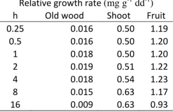
22Testing physiological assumptions
23Relative growth rate (RGR) of shoots in the Fuji tree structure at M scale increased with the 24
values of the friction parameter while, for fruits and old wood, it increased for h values from 0.25 to 25
respectively 4 and 2, and then decreased until a value of 16 (Table 3). In other terms, the higher the 26
values of the friction parameter the higher was the growth occurring close to the C-source. RGRs of 27
old wood and shoots were comprised between normal growth observed in the field and maximum 28
potential growth data used for calibration of sink demands (between 5.3*10-3 and 3.1 *10-2 mg/g for 29
the old wood, between 0.4 and 1.2 mg/g for shoots; Reyes et al. 2016). Conversely, fruit growth 30
was between 35% and 51% lower in respect to the fruit growth observed in the normal field 31
conditions (1.9 and 2.8 mg/g for fruits). 32
13
Simulation results at M scale show the impact of the friction parameter (h) in determining 1
the area around an individual fruit within which this competes for C-assimilates with other fruits 2
(Fig.4A, B). As shown by the significant correlations among fruit growth and comfort index (ratio 3
between C-assimilated and number of fruits), the neighborhood within which fruit growth is 4
affected by competition for C is relatively large (>0.9 m) for small values of the friction parameter 5
(0.5 - 4). This means that the within-tree variability in fruit growth is mostly related to C-sources 6
located far from it. In other terms, a large part of the tree structure affects the growth of each 7
individual fruit. Conversely, for high friction parameter values (8, 16), fruit growth is affected 8
mainly by the C provided by close leaves and possibly the competition with neighboring fruits 9
(neighborhood < 0.9 m) (Fig.4B). 10
The normalized fruit dry weight simulated on the four-year old Fuji tree was compared to 11
that of fruits measured at harvest in a two similar trees, in order to evaluate what range of the 12
friction parameter best fit the observed fruit size distribution (Fig.4C). The lowest RMSE values 13
were obtained with h parameter values between 4 and 16. High values, however, produced skewed 14
distributions with variability larger than the one obtained in the field (h = 16). Conversely, for low h 15
values (0.5, 1) distributions had a consistently lower variability than in the field. Similar variability 16
and low RMSE values were obtained with the friction parameter values of four and eight. 17
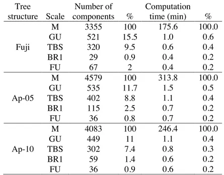
C-allocation at multiple scales
18Changing the scale of representation of the tree from M to coarser scales sharply decreased 19
the number of represented topological components of the tree structures. Trees at GU, TBS, BR1 20
and FU scales contained respectively about 12.7%, 8.6%, 1.6%, and 1.2% the elements they had at 21
M scale (Table 4). 22
Changing topological scale had also a significant impact on fruit growth. In order to ease the 23
interpretation, and based on the above fitted values, only results for the best friction parameter 24
values (2 <= h <= 8) are presented. Fruit growth at GU and TBS scales was more correlated to 25
results at M scale than at coarser scales (BR1, FU) (Fig.5). Generally, in simulations at coarse 26
scales, fruit growth predictions was lower in respect to the M scale. For instance, when running the 27
simulations at FU scale, differences in mean fruit dry weight compared to those obtained at M scale 28
(used in the PEACH model, Allen et al. 2005) went up to 60% in terms of coefficient of variation of 29
the RMSE (Fig.6B). 30
As expected, multiple fruits belonging to the same coarse scale component had the same 31
growth (size of spheres on Fig.3). This was due to the facts that that all fruits at the beginning of the 32
simulation had identical weight and that the carbon allocated to a coarse scale component is 33
proportionally divided according to individual metamer carbon demand. As a consequence, the 34
14
higher the resolution in representing the plant structure (Metamer > Growth Unit > TBS > 1st order 1
Branching ≈ Fruiting Unit), the higher number of different fruit growth achieved (Fig.5). Globally, 2
the lower the friction parameter the lower the range of fruit growth variability, in all the tree 3
structures and at all topological scales (Fig.4C, Fig.5D). The corollary of these observations is high 4
values of the friction parameters result in a relatively wide range of fruit growth at all scales, but 5
with lower within-tree variability when moving from a M to a coarse scale. 6
Simplification of the tree structures and computation efficiency
7Computation time was found as a third order polynomial function of the number of 8
components in the plant (Supplementary Information - Fig.1). The reduction in the number of 9
represented plant components, obtained by changing scale from M to FU (down to 0.8%) in the 10
presented simulations, resulted in a gain in computation time of up to four orders of magnitude 11
(down to 0.2%) (Table 4). 12
The reduction in computation time associated with the use of coarser scales (Table 4) 13
corresponded to an increased discrepancy (in terms of the Coefficient of Variation of the Root 14
Mean Squared Error: CV RMSE) in the results obtained between M and other scales (Fig.6B). Error 15
varied from values next to zero at low friction parameters at GU scale, to values up to sixty percent 16
for higher frictions and BR1 or GU scales, and was generally higher for higher fiction parameter 17
values. There were however minor exceptions to this general behavior, with low friction parameter 18
values occasionally providing slightly higher discrepancies than higher values (e.g. for h = 4 at 19
BR1 scale in the Ap-05 and Ap-10 tree structure, in respect to h = 8). 20
DISCUSSION
21Multi-scale coherence, impact on predictions and computation time
22To our knowledge, MuSCA is the first allocation model that allows simulating C-23
allocation at multiple topological scales within a plant representation. Simulation results revealed 24
that the model was able to produce results which are highly correlated with the M scale, especially 25
when running at GU scale (Fig.5). As a rule of thumb, the deviation between predictions obtained at 26
M and other scales increased when up-scaling and for increasing friction parameter values (Fig.5, 27
Fig.6). 28
Differences in C allocated to fruits at M and other scales are due to two factors. Firstly, after 29
allocation, the C received by the different plant parts belonging to a component is no longer 30
influenced by their individual positions. As such, the model represents the effects of distances 31
among the components at the coarse scale selected for the simulation, but not among its constituting 32
15
elements at the finer scale. Second, while the top and basal coordinates of a coarse scale component 1
are inherited from the finer scale components present at its extremities, the coordinates of its 2
barycentre are not. Indeed these are computed as the mean of the coordinates of its components, 3
weighted by their individual lengths. When distances and C-flows are calculated, this generates 4
deviations in respect to the M scale 5
The deviations between M and other scales were also affected by the specific plant structure 6
(Fig.5). This is likely related to the non-linearity of the simulated process and its relation to the 7
different discretization of the plant. In trees, the different contribution in respect to the available C 8
of annual organs (leaves and fruits) and the presence of the moderate C-sink of woody organs may 9
create contrasting patches in terms of C-supplies and C-sinks (Fig.4). When the tree is discretized at 10
different scales, the distances between patches of sources and sinks and their constituting elements 11
are modified. By changing discretization, the set of distances to which the non-linear function (eq. 12
1) is applied to compute C flows also changes, implying sharp differences in C-allocation. Changes 13
are thus related to the geometry of the tree structure as well as to the specific friction parameter, as 14
they determine the spatial domain and the impact of the C-allocation rule. In this regard, further 15
research would be required to explore the impact of commonly applied equations for C-allocation 16
(e.g. eq. 1, equations in Balandier et al. 2000; Lescourret et al. 2011) on tree architectures 17
contrasting in terms of distributions of sinks and supplies in relation to their discretization. 18
Changing topological scale also had a strong impact on the computation time. This is an 19
important limiting factor for the simulation of carbon allocation in complex tree structures, and 20
consequently simulations of tree growth at high spatial detail tends to be limited to relatively young 21
plants (Balandier et al. 2000; Pallas et al. 2016). Computation time in MuSCA closely 22
approximates a third order polynomial function of the number of represented plant components 23
(Supplementary Information - Fig.1), suggesting the need to reduce plant complexity to simulate 24
plant growth with this type of source-sink model. In this study, the GU scale was able to reproduce 25
values and fruit growth distributions almost identical to M, while saving computation time (Fig.5, 26
Fig.6). It is possible that the optimal scale of representation may be influenced by tree size. Because 27
of the exponential increase in tree topological complexity with tree age, relatively small variations 28
in C-dynamics in early growth stages may have important consequences for the development of the 29
tree structure at later stages. We propose the hypothesis that intermediate scales comprised between 30
M and GU may further decrease the deviations in respect to M scale. We further suggest that a 31
mixed use of high and relatively low topological resolutions, respectively for young and older trees, 32
may optimize prediction accuracy while still allowing for simulations on mature trees. 33
16
Testing physiological assumptions
1
The formalization used in MuSCA to calculate C-allocation (eq. 1a) (Balandier et al. 2000) 2
represented the impact of C-availability and competition among sinks, such as the fruits (Fig.4) on 3
fruit growth variability. 4
RGRs at compartment level was lower range of field observations. This is due to the choice 5
for simulations of a partly cloudy day, in which C-assimilation could limit growth, resulting in 6
enhanced competition for C (whereas simulations in very sunny days resulted in higher growth and 7
reduced fruit growth variability, data not shown). 8
In MuSCA, the considered friction parameter (h, eq. 1) is empirical and does not correspond 9
to a clear biological process. As in previous studies, this parameter has been estimated by trial and 10
error (Balandier et al. 2000). Nonetheless, the comparison between the simulated and harvested 11
normalized fruit growth distribution suggests that h values should be between four and eight 12
(Fig.4C). This suggests that neither a common assimilate pool (Heuvelink 1995) of carbon nor a 13
shoot or branch autonomy (Sprugel et al. 1991) was adequate for accounting for assimilate 14
partitioning within a fruit tree as observed in previous experimental studies (Walcroft et al. 2004; 15
Volpe et al. 2008). Moreover, fluxes from parts of trees with high carbon supply to parts with a low 16
one have already been used for modeling the within-tree variation in fruit size in peach and apple 17
trees (Lescourret et al. 2011; Pallas et al., 2016). Nevertheless, it has also been observed that the 18
level of shoot or branch autonomy can vary depending on the phenological date with a higher 19
branch autonomy during summer period compared to winter (Lacointe et al. 2004). Further 20
simulations and analyses with MuSCA performed by dynamically tuning the friction parameter 21
values could help testing such behaviors. 22
Advantages of flexible C-allocation at multiple-scales
23By making a dynamic use of MTG (Godin and Caraglio 1998) the presented model allows 24
us modifying the type of “individual entities” considered in source-sink exchanges within a plant 25
structure on the fly. This is also made possible by formalisms which are equally applicable at all 26
scales (Fig.2, eq. 2, 3) and inherit, from fine to coarse scales, the spatial (coordinates of scale 27
boundaries) and extensive (C-demands and supplies, Up- and down- scaling) properties necessary 28
for the calculation of C-flows. 29
The flexibility related to the multi-scale features of the model provides several opportunities. 30
While the topological scale typically represented in a plant models mirrors the interests of a 31
particular group of model users, changing the scale of representation makes the model of practical 32
interest for multiple objectives. As showed in this study, the model can be used to assess the 33
implications of using specific scales. From our results, in most cases and for trees of this size, the 34
17
GU scale would be a robust alternative to M, while allowing much faster simulations. Comparisons 1
of results among C-allocation models could be facilitated by adapting the scale of representation. 2
For instance, the individual fruit growth simulated at the FU scale can be compared with results 3
obtained by QualiTree (Lescourret et al. 2011). 4
In this study, MuSCA was applied on MTGs issued from the MAppleT architectural model 5
(Costes et al. 2008). However, MTGs coming from other sources, such as the several models 6
present in the OpenAlea environment, could also be used, given their compliance with certain 7
prerequisites. Also, the detail in the description of the plant could be less detailed since, technically, 8
a representation at metamer resolution is not strictly necessary. Indeed, in order to run MuSCA, the 9
plant description should simply allow for the identification of the organ types (via the presence of 10
leaves and fruits), their geometrical sizes (length and radiuses) and their topological connections 11
(succession, branching). This makes the model applicable on tree structures acquired in the field by 12
methods such as the Terrestrial Laser Scanner (TLS), followed by topological reconstruction of the 13
plant (Raumonen et al. 2013; Boudon et al. 2014; Reyes 2016). In addition, field data collected at 14
various topological scales might still be suitable for model testing. Indeed, by using the up- and 15
down-scaling, results simulated at any spatial scale can be brought to the scale at which the data for 16
validation are available. 17
Model limitations and further developments
18MuSCA still neglects to represent some important physiological implication of the 19
distribution of sinks along the plant topology. In particular, the influence of individual sinks present 20
in the path between sources and sinks on the C-flow is not fully described, as in models based on an 21
electric analogy and the L-system formalisms (Allen et al. 2005; Cieslak et al. 2011). Indeed, two 22
identical C-sinks (D1, D2) present at the same distance from a source (S) will receive form this 23
source an identical amount of C, no matter if along the path between S and D1 there are stronger or 24
more abundant C-sinks than along the path between S and D2. Nevertheless, simple models as our 25
have the advantage to require the calibration of one parameter only compared to these previous 26
approaches. 27
It is important to remember that like other carbon allocation models applicable to large plant 28
structures, MuSCA makes use of an empirical parameter (the friction parameter). In this study we 29
identified a range of possibly sound parameter values, but more appropriate ones could be 30
experimentally estimated from measurements of the sap flow through marked isotopic carbon 31
(Hansen 1967), as well as measurements of fruit growth in simple tree structures with modified fruit 32
loads. 33
18
The MuSCA model could be further refined by using the MTG properties to increase the 1
computational efficiency without losing prediction accuracy. For instance, when running at coarse 2
scale, the direction of origin of C-assimilates might be used to account for distance also within the 3
boundaries of the coarse scale component. 4
The creation of new metamers should be included in order to allow for the simulation of 5
plant growth during elongation and growth periods (on not-fixed structures). In addition, given the 6
influence of pruning on the distribution and emergence of carbon sinks, the implementation of a 7
module describing reactions to this management practice (e.g. DeJong et al. 2012) would 8
significantly extend the applicability of the model to a broader range of real cases. Further, a more 9
detailed description of the root would be the starting point to investigate water and nutrient 10
limitations at the soil interface. 11
Regarding the use of MuSCA in the larger context, its generality can ease its adaptation to 12
different species. In addition, the modular implementation of MuSCA in the OpenAlea environment 13
facilitates the integration with other, previously developed, models, as it was the case for the 14
connection with the MAppleT (Costes et al. 2008) and the RATP models (Da Silva, Han, and 15
Costes 2014). 16
CONCLUSIONS
17In this study we presented MuSCA, to our knowledge the first C-allocation model allowing 18
to simulate C-allocation at multiple topological scales of representation of the plant. The presented 19
model provides topologically-based methods to re-interpret/simplify the topological scale at which 20
the process of carbon allocation is simulated. The simulations revealed a major impact of the 21
topological scale, used to discretize C-sources and sinks, on the predicted C-allocation, even when 22
other C-allocation rules (equation for C-allocation and friction parameter) were kept constant. The 23
model can be used to identify which degree of simplification is acceptable for the representation of 24
plant structures without compromising the accuracy in the computation of carbon allocation. It can 25
be used on large plants, being aware of the trades-off in terms of computation time and prediction 26
accuracy. In addition, the flexible representation of the plant topology facilitates matching the needs 27
of different users, while using the same model. For instance, a relatively coarse scale (e.g. branch) 28
could be more suited for a farmer interested in fruit thinning, than a fine one (e.g. metamer) that 29
could be the target of a modeler interested in investigating the local drivers of individual fruit size 30
variability. 31
19
ACKNOWLEDGEMENTS
1
We acknowledge Jerome Ngao and Marc Saudreau from UMR PIAF, INRA at Clermont-2
Ferrand respectively for their help in linking RATP to MAppleT and in linking MTG and RATP, in 3
the OpenAlea platform. F. Boudon from UMR AGAP, Cirad at Montpellier, for some tips on 4
Python coding. The authors thank also Roberto Zampedri and Mr Mauro Cavagna for field 5
assistance, Maddalena Campi for useful discussions, and Gareth Linsmith for supervision on the 6
English language and kinship. 7
FUNDING INFORMATION
8This work was financed by the FIRST FEM doctoral school, which is funded by the 9
Autonomous Province of Trento, Italy. 10
LITERATURE CITED
11Allen MT, Prusinkiewicz P, DeJong TM. 2005. Using L-systems for modeling source-sink
12
interactions, architecture and physiology of growing trees: the L-PEACH model. New Phytologist 13
166: 869–880.
14
Balandier P, Lacointe A, Le Roux X, Sinoquet H, Cruiziat P, Le Dizès S. 2000. SIMWAL: a
15
structural-functional model simulating single walnut tree growth in response to climate and pruning. 16
Annals of Forest Science 57: 571–585.
17
Balduzzi M, Binder BM, Bucksch A, et al. 2017. Reshaping plant biology: qualitative and
18
quantitative descriptors for plant morphology. Frontiers in Plant Science 8. 19
Bancal P. 2002. Source-sink partitioning. Do we need Munch? Journal of Experimental Botany 53:
20
1919–1928. 21
Barillot R, Chambon C, Fournier C, Combes D, Pradal C, Andrieu B. 2018. Investigation of
22
complex canopies with a functional–structural plant model as exemplified by leaf inclination effect 23
on the functioning of pure and mixed stands of wheat during grain filling. Annals of Botany 123: 24
727–742. 25
Barthélémy D. 1991. Levels of organization and repetition phenomena in seed plants. Acta
26
Biotheoretica 39: 309–323.
27
Barthélémy D, Caraglio Y. 2007. Plant architecture: a dynamic, multilevel and comprehensive
28
approach to plant form, structure and ontogeny. Annals of Botany 99: 375–407. 29
Boudon F, Preuksakarn C, Ferraro P, et al. 2014. Quantitative assessment of automatic
30
reconstructions of branching systems obtained from laser scanning. Annals of Botany 114: 853–862. 31
Cieslak M, Seleznyova AN, Hanan J. 2011. A functional–structural kiwifruit vine model
32
integrating architecture, carbon dynamics and effects of the environment. Annals of Botany 107: 33
747–764. 34
20
Costes E, Sinoquet H, Kelner JJ, Godin C. 2003. Exploring within‐tree architectural development
1
of two apple tree cultivars over 6 years. Annals of Botany 91: 91–104. 2
Costes E, Smith C, Renton M, Guédon Y, Prusinkiewicz P, Godin C. 2008. MAppleT:
3
simulation of apple tree development using mixed stochastic and biomechanical models. Functional 4
Plant Biology 35: 936.
5
Da Silva D, Han L, Costes E. 2014. Light interception efficiency of apple trees: A multiscale
6
computational study based on MAppleT. Ecological Modelling 290: 45–53. 7
Da Silva D, Han L, Faivre R, Costes E. 2014. Influence of the variation of geometrical and
8
topological traits on light interception efficiency of apple trees: sensitivity analysis and 9
metamodelling for ideotype definition. Annals of Botany 114: 739–752. 10
Davidson RL. 1969. Effect of root/leaf temperature differentials on root/shoot ratios in some
11
pasture grasses and clover. Annals of Botany 33: 561–569. 12
De Schepper V, De Swaef T, Bauweraerts I, Steppe K. 2013. Phloem transport: a review of
13
mechanisms and controls. Journal of Experimental Botany 64: 4839–4850. 14
De Swaef T, Driever SM, Van Meulebroek L, Vanhaecke L, Marcelis LFM, Steppe K. 2013.
15
Understanding the effect of carbon status on stem diameter variations. Annals of Botany 111: 31-46
16 17
DeJong TM, Negron C, Favreau R, et al. 2012. Using concepts of shoot growth and architecture
18
to understand and predict responses of peach trees to pruning. Acta Horticulturae: 225–232. 19
Fournier C, Pradal C, Louarn G, et al. 2010. Building modular FSPM under OpenAlea: concepts
20
and applications In: Davis, CA, United States, 109–112. 21
Garin G, Fournier C, Andrieu B, Houlès V, Robert C, Pradal C. 2014. A modelling framework
22
to simulate foliar fungal epidemics using functional–structural plant models. Annals of Botany 114: 23
795–812. 24
Garin G, Pradal C, Fournier C, Claessen D, Houlès V, Robert C. 2018. Modelling interaction
25
dynamics between two foliar pathogens in wheat: a multi-scale approach. Annals of Botany 121: 26
927–940. 27
Génard M, Dauzat J, Franck N, et al. 2008. Carbon allocation in fruit trees: from theory to
28
modelling. Trees 22: 269–282. 29
Godin C, Caraglio Y. 1998. A multiscale model of plant topological structures. Journal of
30
Theoretical Biology 191: 1–46.
31
Grechi I, Vivin Ph, Hilbert G, Milin S, Robert T, Gaudillère J-P. 2007. Effect of light and
32
nitrogen supply on internal C:N balance and control of root-to-shoot biomass allocation in 33
grapevine. Environmental and Experimental Botany 59: 139–149. 34
Grossman YL, DeJong TM. 1994. PEACH: a simulation model of reproductive and vegetative
35
growth in peach trees. Tree Physiology 14: 329–345. 36
Grossman YL, DeJong TM. 1995. Maximum fruit growth potential and seasonal patterns of
37
resource dynamics during peach growth. Annals of Botany 75: 553–560. 38
21
Guo Y, Ma Y, Zhan Z, et al. 2006. Parameter optimization and field validation of the functional–
1
structural model GREENLAB for maize. Annals of Botany 97: 217–230. 2
Hansen P. 1967. 14C-Studies on Apple Trees. II. Distribution of Photosynthates from Top and
3
Base Leaves from Extension Shoots. Physiologia Plantarum 20: 720–725. 4
Heuvelink E. 1995. Dry matter partitioning in a tomato plant: one common assimilate pool?
5
Journal of Experimental Botany 46: 1025–1033.
6
Hunt R. 1982. Plant growth curves: the functional approach to plant growth analysis. London:
7
Edward Arnold. 8
Kang M, Evers JB, Vos J, de Reffye P. 2008. The derivation of sink functions of wheat organs
9
using the GREENLAB model. Annals of Botany 101: 1099–1108. 10
Lacointe A. 2000. Carbon allocation among tree organs: a review of basic processes and
11
representation in functional-structural tree models. Annals of Forest Science 57: 521–533. 12
Lacointe A, Deleens E, Ameglio T, et al. 2004. Testing the branch autonomy theory: a 13C/14C
13
double-labelling experiment on differentially shaded branches. Plant, Cell and Environment 27: 14
1159–1168. 15
Lakso AN, Johnson RS. 1990. A simpified dry matter production model for apple using automatic
16
programming simulation software In: Acta Horticulturae.141–148. 17
Le Roux X, Lacointe A, Escobar-Gutiérrez A, Le Dizès S. 2001. Carbon-based models of
18
individual tree growth: a critical appraisal. Annals of Forest Science 58: 469–506. 19
Lescourret F, Moitrier N, Valsesia P, Génard M. 2011. QualiTree, a virtual fruit tree to study the
20
management of fruit quality. I. Model development. Trees 25: 519–530. 21
Lobet G, Pound MP, Diener J, et al. 2015. Root system markup language: toward a unified root
22
architecture description language. Plant Physiology 167: 617–627. 23
Luquet D, Dingkuhn M, Kim H, Tambour L, Clement-Vidal A. 2006. EcoMeristem, a model of
24
morphogenesis and competition among sinks in rice. 1. Concept, validation and sensitivity analysis. 25
Functional Plant Biology 33: 309–323.
26
Marcelis LFM. 1996. Sink strength as a determinant of dry matter partitioning in the whole plant.
27
Journal of Experimental Botany 47: 1281–1291.
28
Massonnet C, Regnard JL, Costes E, Sinoquet H, Ameglio T. 2006. Parametrization of the
29
functional-structural model for apple trees. Application to simulate photosynthesis and transpiration 30
of fruiting branches In: Acta Horticulturae. Denmark: ISHS, . 31
Münch E. 1930. Die Stoffbewegunen in der Pflanze. Jena.
32
Ndour A, Vadez V, Pradal C, Lucas M. 2017. Virtual plants need water too: functional-structural
33
root system models in the context of drought tolerance breeding. Frontiers in Plant Science 8. 34
Pallas B, Da Silva D, Valsesia P, et al. 2016. Simulation of carbon allocation and organ growth
35
variability in apple tree by connecting architectural and source–sink models. Annals of Botany 118: 36
317–330. 37
22
Pradal C, Boudon F, Nouguier C, Chopard J, Godin C. 2009. PlantGL: a Python-based
1
geometric library for 3D plant modelling at different scales. Graphical models 71: 1–21. 2
Pradal C, Dufour-Kowalski S, Boudon F, Fournier C, Godin C. 2008. OpenAlea: a visual
3
programming and component-based software platform for plant modelling. Functional Plant 4
Biology 35: 751.
5
Pradal C, Fournier C, Valduriez P, Cohen-Boulakia S. 2015. OpenAlea: scientific workflows
6
combining data analysis and simulation. ACM SSDBM 15: 11–17. 7
Raumonen P, Kaasalainen M, Åkerblom M, et al. 2013. Fast automatic precision tree models
8
from terrestrial laser scanner data. Remote Sensing 5: 491–520. 9
Reyes F. 2016. Carbon allocation of the apple tree: from field experiment to computer modelling.
10
PhD Thesis, University of Bolzano, Italy. 11
Reyes F, DeJong T, Franceschi P, Tagliavini M, Gianelle D. 2016. Maximum growth potential
12
and periods of resource limitation in apple tree. Frontiers in Plant Science 7. 13
Robert C, Garin G, Abichou M, Houlès V, Pradal C, Fournier C. 2018. Plant architecture and
14
foliar senescence impact the race between wheat growth and Zymoseptoria tritici epidemics. Annals 15
of Botany 121: 975–989.
16
Ryan MG, Asao S. 2014. Phloem transport in trees. Tree Physiology 34: 1–4.
17
Sinoquet H, Le Roux X, Adam B, Ameglio T, Daudet FA. 2001. RATP: a model for simulating
18
the spatial distribution of radiation absorption, transpiration and photosynthesis within canopies: 19
application to an isolated tree crown. Plant, Cell and Environment 24: 395–406. 20
Sprugel DG, Hinckley TM, Schaap W. 1991. The theory and practice of branch autonomy.
21
Annual Review of Ecology and Systematics 22: 309–334.
22
Stanley CJ, Tustin DS, Lupton GB, Mcartney S, Cashmore WM, Silva HND. 2000. Towards
23
understanding the role of temperature in apple fruit growth responses in three geographical regions 24
within New Zealand. The Journal of Horticultural Science and Biotechnology 75: 413–422. 25
Thornley JHM, Johnson IR. 1990. Plant and crop modelling. NY: The Blackburn Press.
26
Thorpe M, Minchin P, Gould N, McQueen J. 2005. 10 - The stem apoplast: a potential
27
communication channel in plant growth regulation In: Zwieniecki MA, ed. Physiological Ecology. 28
Vascular Transport in Plants. Burlington: Academic Press, 201–220.
29
Volpe G, Lo Bianco R, Rieger M. 2008. Carbon autonomy of peach shoots determined by
13C-30
photoassimilate transport. Tree Physiology 28: 1805–1812. 31
Vos J, Evers JB, Buck-Sorlin GH, Andrieu B, Chelle M, de Visser PHB. 2010. Functional–
32
structural plant modelling: a new versatile tool in crop science. Journal of Experimental Botany 61: 33
2101–2115. 34
Walcroft AS, Lescourret F, Genard M, Sinoquet H, Le Roux X, Dones N. 2004. Does
35
variability in shoot carbon assimilation within the tree crown explain variability in peach fruit 36
growth? Tree Physiology 24: 313–322. 37