Application of the design structure matrix : a case study in process improvement dynamics

(1)

Application of the Design Structure Matrix: A Case Study in

Process Improvement Dynamics

by

Cory J. Welch

B.S. in Mechanical Engineering Cornell University, Ithaca, NY 1994

Submitted to the Alfred P. Sloan School of Management and the School of Engineering in partial fulfillment of the requirements for the degrees of

Master of Business Administration BARKER

and BRE

Master of Science in Mechanical Engineering MASSAC HRUSTS- -N"TI tb

OF TECHNOLOGY

in conjunction with the

Leaders for Manufacturing Program

at the LIBRARIES

Massachusetts Institute of Technology June 2001

Author

( Sloan School of Management Department of Mechanical Engineering May 11, 2000 Certified

by

John D. Sterman, Thesis Advisor J. Spencer Standish Professor of Management Certified

by

Daniel E. Wh it yJIis Advisor Sepiir Research Scientist Accepted

by

Margaret Andrews, Director of Master's Program jwm &rlol of Management Accepted

by

Ain Sonin, Chairman, DepartdCfdommittee for Graduate Students Department of Mechanical Engineering

(2)

(3)

Application of the Design Structure Matrix: A Case Study in

Process Improvement Dynamics

by Cory J. Welch

Submitted to the Alfred P. Sloan School of Management and the Department of Mechanical Engineering

on May 11, 2001

in partial fulfillment of the requirements for the degrees of Master of Business Administration

and Master of Science in Mechanical Engineering

Abstract

A challenging aspect of managing the development of complex products is the notion of design iteration, or rework, which is inherent in the design process. An increasingly popular method to account for iteration in the design process is the design structure matrix (DSM). This paper presents an application of DSM methods to a novel product-development project. To model the project appropriately, the DSM method was extended in two ways. First, the model developed here explicitly includes overlapping activity start and end times (allowing concurrent development to be modeled). Second, the model includes explicit learning-by-doing (reducing the probability of rework with each iteration). The model is tested on a

subset of the tasks in a complex new product developed by the Advanced Technology Vehicles division of General Motors, specifically the thermal management system of an

electric vehicle. Sensitivity analysis is used to identify the drivers of project duration and variability and to identify opportunities for design process improvement. The model is also used to evaluate potential design process modifications.

Thesis Advisors: John D. Sterman, J. Spencer Standish Professor of Management Daniel E. Whitney, Senior Research Scientist

(4)

Acknowledgements

Completion of this thesis would not have been possible were it not for the support of dozens of people. First, I want to thank my best friend, Sara Metcalf. I cannot overemphasize the value of your emotional and intellectual support during this process. I could not possibly have done this without you. I am also grateful for the support of my mother, MaryAnn, who has encouraged me in all my endeavors and who has always been there for me. I pray your health returns to you. Special thanks are also in order for the rest of my family: Kellie for her friendship; Dad for his words of wisdom; Carol, Jenny, Ryan, Tim, and Nana for their

encouragement; and last, but certainly not least, Bill for being a pillar of support for my ailing mother. I would also like to extend my sincere gratitude to my management advisor, John Sterman, who has given me the gift of a new way of thinking and who has profoundly influenced me -- more than he will probably ever know. Thanks also go to my engineering advisor, Daniel Whitney, for his patient guidance.

I also must express appreciation for my friends in the LFM program, who will all be missed sorely after June. Additionally, I want to thank all those at the Advanced Technology Vehicle division of General Motors who helped make this project possible, especially Greg, Gary, and Bill. I also appreciate the help of many others at the company, including Cara, Mike, Robb, June, Lori, Don, Aman, Andy, Cinde, Bob, Eric, Kris, Mark V., Tom E., Bruce, Ron, Ray, Jim, Jill, Erin, Tom C., Mark S., Steve, Lawrence, Bill, Brendan, and Bob. Finally, I want to thank the Leaders for Manufacturing program at MIT for their support of this work.

(5)

Table of Figures

Figure 2-1 Interaction M atrix ... 14

Figure 2-2 Rework Probability Matrix... 15

Figure 2-3 Rew ork Im pact M atrix ... 16

Figure 2-4 Triangular Distribution of Task Duration ... 17

Figure 2-5 O verlap M atrix ... 19

Figure 2-6 Partial Overlap Illustration ... 20

Figure 2-7 External Precedence Concurrence (adapted from Ford and Sterman, 1998)... 22

Figure 2-8 Learning Curve ... 26

Figure 2-9 Effect of Learning Curve on Project Completion Time... 27

Figure 3-1 Gantt Chart of Baseline Process without Rework ... 29

Figure 3-2 Gantt Chart of Baseline Process with Rework ... 30

Figure 3-3 Baseline Process Completion Time Distributions ... 31

Figure 3-4 Baseline Process: Row Sensitivity Analysis ... 34

Figure 3-5 Cumulative Distribution Function of Baseline and Modified Processes... 38

Figure 3-6 50% Reduction in Rework Probabilities ... 41

Figure 3-7 100 % Increase in Rework Probabilities ... 42

Figure 4-1 Usefulness Constrained by Data Accuracy ... 45

Figure 4-2 Employee Pull and Resistance... 47

(7)

1. Introduction

Technology companies are realizing that the processes they follow in developing their products are themselves a source of competitive advantage. Thus, an increasing amount of attention is being paid to the design and effective management of product development processes (Ulrich and Eppinger, 2000; Wheelwright and Clark, 1992). One challenging aspect of managing the development of complex products is the notion of design iteration, or rework, which is inherent in the design process (Eppinger et al., 1994; Eppinger et al., 1997; Smith and Eppinger, 1997a; Smith and Eppinger, 1997b; Steward, 1981). Osborne (1993) discovered that between one third and two thirds of total development time at one

semiconductor firm was a result of design iteration. Since substantial savings could be realized by minimizing the amount of rework in the design process, it is desirable to have

management methodologies that consider rework. Unfortunately, conventional management techniques such as Gantt charts and PERT/CPM are unable to account for design iteration. One method of explicitly accounting for iteration in the design process that is increasingly used is the design structure matrix (DSM)2

The design structure matrix was developed by Steward (198 1a, 198 1b), who described how DSM could be used to identify iterative circuits in the design process and suggested means to manage these circuits, such as optimally sequencing design tasks to minimize iteration. Subsequently, much work has been done to develop the DSM methodology. Black (1990) applied DSM to an automotive brake system in an attempt to optimize the design process. Smith and Eppinger (1 997a) presented a DSM model that uses deterministic task durations

1Project Evaluation and Review Technique/Critical Path Method

(8)

and probabilistic task rework to estimate project duration. They assume, however, that all design tasks are sequential (i.e., no overlapping of design tasks). Smith and Eppinger (1997b) also developed a DSM model representative of a highly concurrent engineering process. Their model assumes that all design tasks are performed in parallel and that rework is a function of work completed in the previous iteration. Additionally, Smith and Eppinger

(1998) describe a model that addresses the question of whether design tasks should be sequential or parallel. Carrascosa, Eppinger and Whitney (1998) describe a DSM model, based largely on work done by Krishnan, Eppinger, and Whitney (1997), that relaxes the

assumption that design tasks are either purely sequential or parallel, permitting partial overlapping of sequential or parallel activities.

Browning (1998) drew upon much of this previous work and developed a DSM simulation model implemented in Microsoft@ Excel and Visual Basic that integrates project cost, schedule and performance. Unlike previous models, Browning's model treats rework probability and rework impact separately, treats task durations as random variables, and applies a learning curve to the duration of reworked tasks. Browning's model permits tasks to be both sequential and parallel, but does not permit partial overlapping of interdependent activities. Additionally, Browning's model is intended for use as a project simulation tool whereas previous models are primarily mathematical in nature.

In this paper, I discuss the application of a portion of Browning's (1998) model to the thermal management system of a battery-powered electric vehicle. I extend Browning's model to permit partial overlapping of interdependent design tasks (allowing concurrent development

(9)

to be modeled). I also modify Browning's algorithm to apply a learning curve to the rework probabilities rather than to the task durations. The goal of the application and model

development was two-fold. First, I developed and evaluated Browning's model for potential use at the Advanced Technology Vehicles division of General Motors. Second, I used the

model to identify opportunities for process improvement and to evaluate design process modifications.

The remainder of this paper is organized as follows. Section 2 introduces the model

developed by Browning (1998) and discusses the modifications I made. Section 3 describes the application of the model, presenting the results of baseline process analysis, sensitivity analysis, and comparison of the baseline design process with a modified design process. Section 4 evaluates the modeling technique and makes suggestions for future use. Section 5

provides concluding remarks.

2. Application of the Design Structure Matrix (DSM)

This section introduces the organization where the study was conducted, describes the design process that I modeled as well as the fundamentals of Browning's (1998) DSM model, and explains the modifications I made to Browning's algorithm.

2.1. Advanced Technology Vehicles

I conducted this study while employed as an intern at the Advanced Technology Vehicles (ATV) division of General Motors. ATV is responsible for the development of alternative propulsion vehicles (e.g., electric and hybrid-electric vehicles) and is an organization that bridges the gap between pure research and development and mass production. Alternative

(10)

propulsion vehicles require much more invention than a typical vehicle development program, and sales volumes are much smaller. Thus, the processes followed are generally less well defined than those for a mass market vehicle. Each vehicle program is typically quite different from the last.

2.2. System Description

The process chosen for analysis was the thermal management system (TMS) of a battery-powered electric vehicle. The TMS maintains component and cabin temperatures within an acceptable range. Components such as batteries, motors, and controllers generate significant heat during operation, which must be dissipated for proper functionality, reliability, and durability. Cabin temperature (the temperature within the passenger compartment of the vehicle) must also be maintained within an acceptable range for customer comfort and satisfaction. The loading of the thermal management system, which in part determines the required system mechanization and component sizing, is highly dependent on characteristics of the components it is responsible for cooling or heating and thus is tightly coupled with the design of the rest of the vehicle. This characteristic of the system makes it a good candidate for evaluation using DSM, which can highlight important interactions in a complex design process.

2.3. Definition of the Process

After selecting the TMS as the process to be modeled, the specific tasks in the design of the system must be identified. To identify the design tasks, I conducted approximately ten one-on-one interviews with the engineers and managers responsible for this system (one design engineer, one test engineer, and one engineering manager). Interviews ranged from thirty

(11)

minutes to two hours. Design tasks were elicited from the engineers and managers with the following guidelines for task identification.

A good DSM process model will:

- _{capture all significant design tasks (if not explicitly, then as a subset of a larger task)} - capture all tasks that could result in design changes (e.g., design reviews)

* capture interactions with other systems

* capture significant transfers of information between tasks and subsystems - have an appropriate level of aggregation.

The last guideline was the most problematic. Too high a level of aggregation runs the risk of producing a model that does not capture important information flows. However, too low a level of aggregation (i.e., having too much design detail) can overwhelm the modeler and the experts with data gathering and parameter estimation for which they have little basis and which might add no value in the end. To mitigate these risks, I started by asking the system experts to identify all design tasks without regard to the level of detail. I then worked with the engineering manager to combine many sub-tasks into larger, aggregate categories. The

resulting DSM includes 19 design tasks (see Appendix 1 for task descriptions). An illustration of the aggregation process is provided in Appendix 2.

2.4. Data Collection and Parameter Estimation

Once the design tasks have been identified, the analyst must work with experts to estimate the rework probabilities, rework impacts, task durations, and task learning curves (see sections

2.5 and 2.6). To ensure that the input data were as accurate as possible, I worked one-on-one

with the engineering manager most knowledgeable about the overall design process. I provided detailed instructions on how to fill out each of the matrices before a series of meetings during which the data were estimated (see Addendum 1 of Appendix 8). Then, I

(12)

met with the manager approximately ten times for meetings ranging between 30 and 90 minutes each to elicit data and estimate parameters. Data on task durations (Appendix 4) were also obtained from other engineers who had worked on past projects.

A difficult aspect of parameter estimation was differentiating between rework probability and rework impact. It became evident that the tendency was to assign the same value for rework impact as for rework probability, effectively lumping the probability and impact of rework into one number. To minimize this effect, I frequently repeated the specific question to be answered for each data value (see Addendum 1 of Appendix 8). Additionally, it was difficult to assign a single value to either rework probability or rework impact. In some cases, there may be a high probability of rework occurring, but the impact may be low. At the same time, there may be a small probability of rework occurring, but the impact may be high. Assigning only one value to rework probability and rework impact was thus difficult. This difficulty might be overcome by instead asking for a range of possible rework probabilities and rework impacts. However, the problem would still exist of potentially having multiple rework probability ranges corresponding with different rework impact ranges. After participating in

all of the data collection, I must emphasize the value of one-on-one meetings, as opposed to surveys. Due to the complexity of the model algorithm and the numerous caveats that go with data estimation (see Addendum 1 of Appendix 8), having a model expert present during data estimation is vital to eliciting reasonable data.

(13)

2.5. Introduction to the DSM model

The model used to analyze the TMS design process was adapted from Browning (1998)3. For simplicity, the model used in this paper focuses on project duration and does not model

project cost or performance (quality), as did Browning's model. In addition to describing the basics of the algorithm developed by Browning, this section also presents refinements of the algorithm. The need for these refinements was discovered in the process of modeling the TMS design process. While the changes were considered necessary to characterize

adequately this particular process, the results are generic enough to be applied to any design process. The modifications could also be incorporated easily into Browning's integrated duration, cost, and quality model.

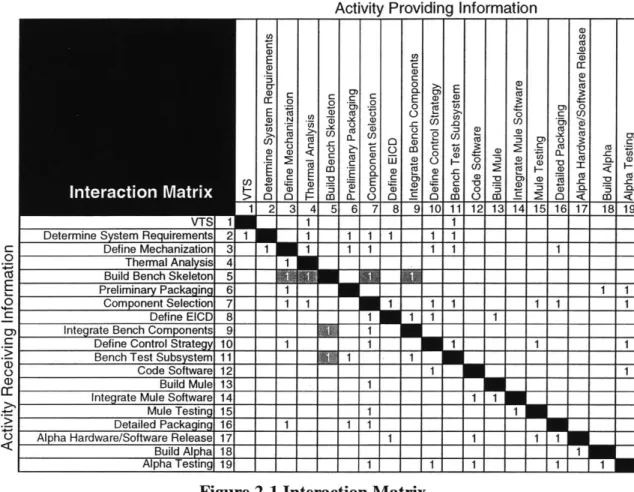
Basic DSM

An "activity-based" DSM is a square matrix that identifies interdependent design activities.4 Figure 2-1 shows the interaction matrix for the thermal management system design process. The presence of a "1" in the cell where two design tasks interact indicates that one task either provides information to or receives informationfrom the other. The rows of the matrix indicate that the task associated with that row receives information from the tasks whose cells contain a one. For example, in Figure 2-1, task 5 (Build Bench Skeleton) is seen to receive

informationfrom tasks 3, 4, 7 and 9. Conversely, the columns of the matrix indicated that the

task associated with that column provides information to the tasks whose cells contain a one. For example, in Figure 2-1, task 5 is seen to provide information to tasks 9 and 11.

3 The model used an Excel spreadsheet interface with Visual Basic macros. The program can be obtained from

the author.

4 Many different kinds of DSM's are used. Examples include component-based, parameter-based, team-based and activity-based DSM's. This model is an example of an activity-based DSM. Additional information on DSM can be found at http://web.mit.edu/dsm/.

(14)

C

Activity Providing Information

co C CO Build~C B(D keeo C~~r D00in EED81 rnt r0t Bec Co nEt -G) 0 0

Define~( Sta C0to U1

Bec Tes Sub 11 Ze 1 M

Cul Muld 13 (D1- 3 a D M T 1) DWaie n Pa.k 12 1)( W 71 14 S0 (D 0 LI M 0 )2-( B(Dl hLT0Xa AE W 000 0 0 0 0 =_ L C

Determine System Requirements 21 1 TIW - 1 1 1 1 1

DefineMechanization 3 1 1 1 1 1 1 1 Thermal Analysis 4 1 1

Build Bench Skeleton

5-E Preliminary Packaging 6 1 11 11 1

RComponent Selection 7T7 1 1 1 1 _ T 1

Integrate Bench Components 9 -_ 1 1

Define Control Strategy 101 1__ -T_ 1 _

Code Software 121_

EIntegrate Mule Software 14 1 1

Mule Testing 15 1 1_

Detailed Packaging 16 1 1 1 ~) Alpha Hardware/Software ReleaseT17 1 1_ _ 1

Build Alpha 18 1 11

Alpha Testing

19---Figure 2-1 Interaction Matrix

Browning's (1998) Model

Browning's (1998) model uses the DSM structure and Monte Carlo simulation to predict the distribution of possible project durations. The model assigns both rework probabilities and rework impacts to each instance where an interdependence between design activities was identified. As an example, the rework probability matrix in Figure 2-2 illustrates that upon completion or rework of task 4, a 50% probability exists that tasks 2 and 3 would have to be reworked, and a 5% probability exists that task 1 would have to be reworked. In general, numbers above the diagonal are estimates of the likelihood that completion of the task in the

same column as that number will cause re-work of the task in the same row as the number. These numbers represent the chances offeedback from one task to another. The numbers below the diagonal have similar meaning, but instead represent a situation offeedforward.

(15)

The presence of a number below the diagonal indicates that there is forward information flow from one task to another. Thus, if the upstream task were re-worked, there is a probability that the downstream task might also have to be re-worked (assuming the downstream task has already started) since the information on which the downstream task is dependent upon would have changed. For example, in Figure 2-2 we see that task 4 provides information forward to tasks 5 and 7. Figure 2-2 illustrates that if tasks 5 and 7 had already started and task 4 had to be reworked, there is a 10% chance that task 5 would have to be reworked and a 50% chance that task 7 would have to be reworked. In general, numbers below the diagonal indicate the likelihood that re-work of the task in the same column as the number will cause subsequent re-work of the task in the same row as the number.

C 0 C E~ C 0 E 0 CD) C 0 CL 0 0. -C.) Ca a) (D 61 71 8 E CD CO U0 CD Ml 9 C 10 Cn (D C: 0 0 11 0 CO ~0 -0 0 0D 121 13 0 0) A CD 0l) 75 Co 141 15 _0 C a 16 aI) a: 0 IS X CIS 0 0. ~0 0) C Cl) 0 I-0 0. 171 181 19 .10 .75 .10 .05 .20 .05 .10 .10 .05 .10 .05 .0 .100 1 j _..0 5 1 _1.051.2013 2 ₁ _.301.1011 0 . 01 1 .0 5 1 _{M .05}.0 5 Define EICD 8 .z . .1 .1__ I I Integrate Bench Components 9 1.0 1.0

Define Control Strategy 10 .80 .20 .80 .20

Bench Test Subsystem 11 1.0 .05 1.0

Code Software 12 1.25

Build Mule 13 .10

Integrate Mule Software 14 1.01.50 Mule Testing 15 .50

Detailed Packaging 16 1.0 1.0 1.0

Alpha Hardware/Software Release 17 1.0 1.0 .10.10M

Build Alpha 18 .25

Alpha Testing 19 .. 10 1.0

(16)

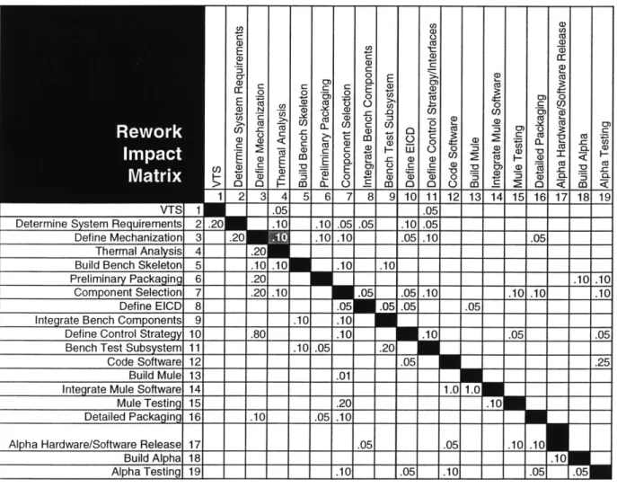
Although rework may be required of a design task, rework of the entire design task may not be necessary. The rework impact matrix in Figure 2-3 provides the fraction of original task duration that would be required in the event that rework was required. For example, the rework impact matrix in Figure 2-3 indicates that an estimated 10% of task 3 would have to be reworked if the Monte Carlo simulation determined that rework of task 3 was required upon completion of task 4. Readers requiring additional detail about how to fill in the rework probability and impact matrices should refer to Addendum 1 of Appendix 8.

C 0 0 CL 0 0. CD C 0 (a. E 0 CD 71 8 .051 .05 .10 E Cn U a) _I-9 0 0 C 10 CO 0 (D ) CD 7) C 0 C: 11 CO 0 12 a) 13 CU 0) C/) 14 0) C CU a) I-a) 0) C (U 0 (U 0~ ~0 a) a) 0 ca 2-CU3 a: cis 151 161 17 (U 0. ca 0) C CU a) I-CU 0. 181 19 1.051 I 1 1 1. 1. 1 .1 .101 .05 .051 .10 .05 Preliminary Packaging 6 .20 .10 .10 Component Selection 7 .20 .10 .05 .05 .10 .10 .10 .10 Define EICD 8 .05 .05.05 .05

Integrate Bench Components 9 .10 .

Define Control Strategy 10 .80 ._ .10 .051 .05

Bench Test Subsystem 11 .10 .05 .20

Code Software 12 .05 .25

Build Mule 13 .01

Integrate Mule Software 14 1.0 1.0

Mule Testing 15 .20 .10

Detailed Packagin 16 .10 .05 .10

Alpha Hardware/Software Release 17 .05 .05 .10 .10

Build Alpha 18 .10

Alpha Testing 19 .10 .05 .10 .05 .05

Figure 2-3 Rework Impact Matrix , ,

| | I || | | | .0 5

(17)

Design task durations are modeled as random variables with triangular distributions for mathematical convenience. Estimates of the most likely value (MLV), best case value

(BCV), and worst case value (WCV) provide the endpoints of the triangular distribution. Figure 2-4 illustrates the probability distribution function of the design task duration as

modeled by Browning (1998). Estimates of the task durations for the TMS design process are provided in Appendix 4.

BCV MLV WCV

Design Task Duration

Figure 2-4 Triangular Distribution of Task Duration

With probabilistic task rework and randomly distributed task durations, output project duration will be a continuous random variable. Monte Carlo simulation is used to predict the distribution of project duration. Readers requiring additional detail on the model algorithm should refer to Browning (1998) or Appendix 7 for the model code.

2.6. Modification of Algorithm

In this section, I describe the modifications made to Browning's (1998) base algorithm. Specifically, I describe modifications permitting task overlap (permitting concurrent

(18)

2.6.1. Task Overlap

While defining the thermal management system design process and gathering data for modeling, it became apparent that simulated design times using Browning's (1998) model were likely to be several fold longer than what they would be in reality. The primary reason was that the algorithm developed by Browning (1998) requires that a downstream task cannot begin until the upstream task on which it is dependent is 100% completed. Browning's

algorithm permits activities to be performed in parallel only if the downstream task does not rely on the upstream task for any information (i.e., no task interdependence). In reality, more

and more programs are designed as concurrent engineering programs. That is, activities dependent on one another proceed, at least to some extent, in parallel and extract information as they progress. While a design task may require information from another upstream design task, it is not always the case that 100% of the upstream task must be completed before the downstream task may commence.

To account for a degree of overlap between tasks that were interdependent, an additional matrix was created. For illustration, the overlap matrix for the TMS is shown in Figure 2-5.

(19)

0) Co) C 0 o a) a) C) U a) c CM 0) E 0 0) C C CD CD .0 o .- o E) 0 00 ~ Co 0) 00 Cu 2 o) C o I' 0 75 C .0 >. a) > U ) CO 0 :3 7- a) a) _ o (I CC~0 - ) a) ) 0a ) Q a) u 5 0D 0 (D ~ < Co a) a a. .Co ( 0)~ C a) i W 0 0 5 0) 2L 6 a) 0 a) )/~ a) _0 < C E C'D -u F- Q)~00) ~ CD a) 3 o - 0) 0 a) 0) ~ ~ W o >00 ma. EL C.MO 0 0 M G~ ~ < Co <

Determine System Requirements1

Define Mechanization 3 .2

Thermal Analysis 4

Build Bench Skeleton 5 Preliminary Packaging 6

0 '4 C 6 7 ₈₀ I4I ID 10 17 10

IIZI

III

til

11 111

.U.

Com onent Selection 7 .20 .50

Define EICD 8 .

Inte rate Bench Com onents 9 1.0 .

Define ConLrol Strate 1 U .0 .2

Bench Test Subs stem 11 1.0 .10 .80

Code Software 12 .50

Build Mule 13 1.0

Inte rate Mule Software 14 1.0 1.0

Mule Testin 15 1.0 11.

Detailed Packa in 16 1.0 1.0 1.0

Al ha Hardware/Software Release 17 1.0 1.0 .3311.0

Build Al ha 18 1.0

Alpha Testing 19 L_1.0_1._1._1._1.

Figure 2-5 Overlap Matrix

Each sub-diagonal cell where an interdependence exists requires an estimation of the degree of overlap between these design tasks. For example, Figure 2-1 shows that task 5 is

dependent on information from task 3. Thus, an estimate of the percentage of task 3 that must be completed before task 5 can commence is required. From Figure 2-5, we see that about 80% of task 3 must be completed before task 5 may begin. Using this matrix, any degree of overlap, from 0-100%, may be specified, unlike the baseline algorithm developed by

Browning, which assumes that 100% of the upstream task must be complete before the dependent downstream task may commence (equivalent to having a "1" in the overlap matrix cells).

00

50

2 9 10 11 12 13 19

(20)

Figure 2-6 illustrates the difference between Browning's model and the model as I have applied it. Figure 2-6a depicts the Gantt chart representation of two design tasks performed purely in sequence, as required by Browning's model if an interdependence exists between these two tasks. Figure 2-6b depicts two purely parallel design tasks. Browning's model only permits this situation when no interdependence exists between the design tasks (i.e., a zero in the matrix cell where the two design tasks overlap). Figure 2-6c, on the other hand, illustrates a situation where two tasks are interdependent (i.e., the downstream task depends on the upstream task), but the downstream task may commence before 100% of the upstream task is completed. This partial overlap scenario illustrates the effect of including the overlap

matrix in the model.

A: Pure Sequential B: Pure Parallel C: Partial Overlap

Figure 2-6 Partial Overlap Illustration

It is worth noting that only sub-diagonal entries exist in the overlap matrix. Since the tasks are listed in chronological order of task start time, super-diagonal elements, if included, would be an estimation of the percentage of a downstream task that would need to be completed before the upstream task rework could commence. While in reality it is quite possible to identify the need for rework before completion of the downstream task, this model does not consider that possibility. The discovery of required rework for upstream tasks is assumed only to occur after the downstream task is completed, consistent with Browning's (1998) formulation.

(21)

While accounting for a degree of overlap between dependent design tasks represents increased model resolution, it should be noted that the method of accounting for overlap is quite simplified for mathematical convenience and ease of data collection. A more realistic representation of the overlap of dependent design tasks in a concurrent engineering situation might be obtained by applying the concepts presented by Ford and Sterman (1998a). Ford and Sterman (1998a) defined "External Process Concurrence" relationships, which are (possibly) nonlinear relationships between the work accomplished in an upstream design phase and the work available to be accomplished in a downstream design phase. Because these relationships can be nonlinear, the optimal degree of parallelism between tasks can change as the tasks progress. Ford and Sterman (1998b) describe a method to estimate these relationships from the participants in a program. While this concept was applied to dependent

design phases, it seems reasonable that it could also be applied to dependent design tasks.

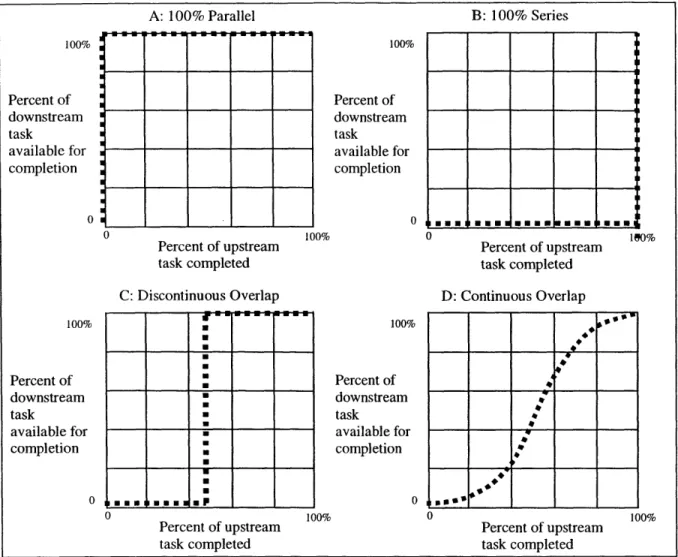
Figure 2-7 illustrates the concept of External Precedence Concurrence relationships. Figure 2-7a portrays a relationship where the downstream task may begin with 0% of the upstream task completed. That is, the tasks are essentially independent. In Browning's (1998) project

model, this situation would represent a case where no interdependence was identified between an upstream and a downstream task. Figure 2-7b illustrates a case where 100% of the

upstream task must be completed before the downstream task may commence. The

relationship portrayed in Figure 2-7b represents the assumed relationship between dependent design tasks in Browning's (1998) project model.

(22)

100% Percent of downstream task available for completion 0i A: 100% Parallel ---0 Percent of upstream task completed C: Discontinuous Overlap 100% Percent of downstream task available for completion 0 100% B: 100% Series 0 1 Percent of upstream task completed D: Continuous Overlap 100% Percent of downstream task available for completion 0 U Percent of upstream task completed 100% Percent of downstream task available for completion 0 100% U Percent of upstream task completed

Figure 2-7 External Precedence Concurrence Sterman, 1998)

(adapted from Ford and

Figure 2-7c, on the other hand, illustrates a relationship between dependent design tasks that is permitted in the project model as I have modified it. This relationship is a discontinuous function, where 100% of the downstream task is available for completion upon completing a certain percentage of the upstream task. Finally, Figure 2-7d illustrates the relationship that is more likely to exist in reality. Figure 2-7d illustrates how, in concurrent engineering

processes, a continuous nonlinear relationship between the percent of downstream task available for completion and the percent of upstream task completed might be represented.

10% U U U ______ U U U U U U U U U U U U U U mu. umu uP ____ 4 4 * 4 ______ 4 _____________ -4--4 4 4 -- 4 4 , ~p ______ ______ ____________ 100%

(23)

While Figure 2-7d, in the author's opinion, more accurately represents the flow of information between interdependent design tasks in a concurrent engineering environment, the added

model complexity and complication of data gathering make using this structure impractical in the DSM model. The relationship shown in Figure 2-7c is considered to be an improvement over the restrictive relationship of Figure 2-7b and is used for simplicity. The reader should refer to Appendix 7 for the code used to model this relationship.

2.6.2. Learning Curve

In addition to the model modification permitting partial task overlap, I also revised the modeling of "learning-by-doing" to permit rework probabilities to be dynamic rather than static. The algorithm developed by Browning (1998) recognized that the nominal duration of a design task might be reduced upon iteration of that design task. The initial design task time may include considerable up front activity, such as setup and gathering of information, that may not have to be repeated if iteration of that design task is required later in the development process. Thus, Browning's algorithm included a subjectively estimated learning factor that represented the percentage of initial task time it would take to perform a design task the second time it is performed during the development process. The model as I applied it, however, did not use this learning curve for three reasons. First, the reduction in effort required for subsequent performance of a task was considered to be accounted for adequately in the rework impact matrix. Second, simulated project durations were relatively insensitive to this learning curve since the reduction in task duration was a one-time step reduction in task time, rather than a fractional reduction with each iteration of the task. Third, I applied a different learning curve, as discussed below, and did not want to overburden participants with data estimation on multiple learning curves.

(24)

Browning's algorithm assumed that the likelihood of reworking a design task would be

constant regardless of the number of iterations of that design task. It has been argued that it is not readily apparent whether the rework probability would increase or decrease with iteration of the task (Smith and Eppinger, 1997). However, observations at ATV indicated that the likelihood of reworking a design task should indeed be reduced with iteration of the design task.

For example, there is an estimated 20% chance that Alpha Testing (see Appendix 1 for a task description and Figure 2-2 for rework probability matrix) may reveal problems with the control logic, requiring the task Define Control Strategy to be reworked. Once these logic errors are identified, the control strategy can be redefined, at which point additional Alpha

Testing will be required to validate the control strategy changes. It seems unreasonable,

however, to assume that upon re-testing, the probability would still be 20% that the control strategy would have to be redefined. Learning has accumulated through the Alpha testing process, and the likelihood of having to redefine the control strategy should now be less. In fact, the reason for these testing stages is to identify problems and reduce the likelihood that the design task has errors that may later become apparent to the customer.

It is well understood that as the rework probabilities approach unity the simulated project duration approaches infinity. The additional work generated by iteration is roughly

proportional to 1/(1-R), where R represents the likelihood that a design task will have to be reworked. Thus, as R approaches unity, the project can never be completed. Consequently,

(25)

estimated project durations are extremely sensitive to any large rework probabilities.

However, discussions with engineers and managers indicated that many instances exist where the likelihood that a task will need to be reworked upon completion of a downstream task,

such as testing, is very high (in some cases nearly 100%) on the first iteration (even in processes that did converge). After learning what was not considered, the likelihood of

iterating that task goes down substantially.

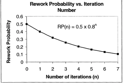
The existence of "learning by doing" is well documented in the literature (Teplitz, 1991)). The simplest reasonable formulation for a rework probability learning curve is to assume the probability of reworking a task falls by a constant fraction with each iteration. Let RPi, = the estimated probability of reworking task i upon completion of downstream task j. Let LCi =

the learning curve assigned to task i, defined as the fractional reduction in rework probability per design task iteration. Let n = the number of times task i is reworked as a result of

completion of task j.5 The equation for the rework probability as a function of the number of

task iterations n is then6 RPi?1 (n) = RP1 (0) * (1- LCi )" , where RPiJ(0) = the estimated

rework probability for the first iteration (see section 2.4 for discussion of parameter estimation).

5 This distinction is important. It means that individual rework probabilities are reduced only upon iteration of the task, as compared with a reduction of the entire row of rework probabilities associated with a task: learning is specific to a task and does not spill over to other tasks.

6 This formulation was only applied to the superdiagonal rework probabilities. Discussion with the engineering manager indicated that these probabilities were less likely to be reduced with iteration of the design task since they represented situations offeedforward rather than feedback. In many cases, the likelihood of reworking the downstream task was 100% if the upstream task was reworked due to strong dependence of the downstream task on the upstream task (as indicated by many subdiagonal l's in the rework probability matrix). Since, in many cases, the 100% value was not likely to be reduced with iteration, a learning curve was not applied to

(26)

Thus, the rework probability will decay exponentially to zero with increasing iteration of the task, as illustrated in Figure 2-87. In the example, RPjj (0) = 0.5 and LC = 0.2.

Figure 2-8 Learning Curve

To estimate the learning curve factors for the TMS design process, I worked directly with the engineering manager. Starting with the estimated rework probabilities for the first iteration, the manager sketched how he thought the rework probability would vary with iteration of the design task. From this sketch, we estimated the learning curve factor that would yield

approximately the same shape as the sketch. Readers requiring additional detail should refer to Appendix 7 for the code used to model this learning curve. Estimates of the learning curve for the TMS design process are provided in Appendix 4.

7 It also might be reasonable to assume that a minimum rework probability, RPmini,, exists and that the rework probability exponentially approaches RPminij rather than zero. The formulation for rework probability would

then be: RP 1 (n) = RP min + (RPj (0) - RP min )* (1 - LCj )" . However, this

formulation would require an additional matrix for the values of RPmini,. In practice, the number of iterations is likely to be small enough that the rework probabilities are not likely to approach zero.

Rework Probability vs. Iteration

Number

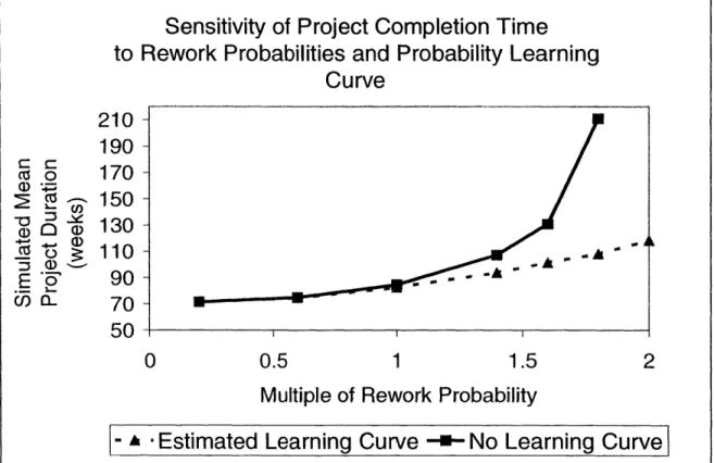
0 .6 -... ... - - .. .. RP(n) = 0.5 x 0.8" 0.4 .0 2 0.3-a. .2 0.2-0 S0.1 0) 0 1 2 3 4 5 6 7 Number of iterations (n)

(27)

Figure 2-9 illustrates the effect that the rework probability learning curve had on simulated project completion time for the TMS design process. Without a learning curve applied to the rework probabilities, project completion time is much more sensitive to uncertainty in the estimated rework probabilities. With no learning curve, project completion times approach infinity with less than a doubling of the estimated rework probabilities (which results in some rework probabilities being near, or equal to unity).

Sensitivity of Project Completion Time

to Rework Probabilities and Probability Learning

Curve

210 - 190-0 170-c ~ 150-( 0 a) 130-0 Z 110-A E f5' 90- -70 -50 0 0.5 1 1.5 2

Multiple of Rework Probability

-

-Estimated

Learning Curve

_--

No Learning Curve

Figure 2-9 Effect of Learning Curve on Project Completion Time

3. Thermal Management System Analysis

This section describes analysis of the TMS design process using the DSM model. I used the model to identify opportunities for improvement in the baseline process and to evaluate potential process changes.

(28)

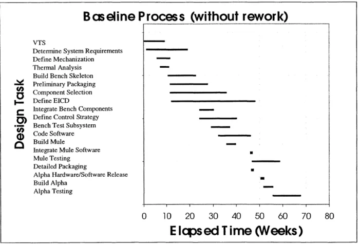
3.1. Baseline Process Analysis 3.1.1. Gantt Charts

After defining the process and gathering the requisite input data, the process may be analyzed for estimated project completion time, project completion time variability, and drivers of project variability. A useful first step in the analysis is to simulate project progression

assuming all tasks are done correctly the first time (no rework). The test was implemented by setting all the rework impact values in the impact matrix to zero8_{. I then generated a Gantt}

chart of the "no rework" case to provide a common sense check of the project simulation9_.

Since most managers are quite familiar with Gantt chart type notation, using a Gantt chart to inspect task ordering, degree of overlap, and project completion time in the event of no rework will help to discover any flawed data points. Further, the simple visual representation will orient the managers to the modeling process and could increase the likelihood that they

will trust the results. The baseline TMS design process with no rework is shown in Figure 3-1.

8 _{It may seem logical to instead assign values of zero to the rework probability matrix. However, the software}

code uses the values in the probability matrix to determine the existence of a precedence relationship. If the entire rework probability matrix were zero, the code would assume that all tasks could be performed in parallel. Assigning a value of zero to the rework impact avoids this effect while never assigning rework during the process.

(29)

Bcseline Process (without rework)

VTS

Determine System Requirements Define Mechanization

Thermal Analysis Build Bench Skeleton Preliminary Packaging Component Selection Define EICD

Integrate Bench Components Define Control Strategy Bench Test Subsystem Code Software

Build Mule

Integrate Mule Software Mule Testing

Detailed Packaging

Alpha Hardware/Software Release

Build Alpha Alpha Testing

0 10 20 30 40 50 60 70 80

E Icpsed T ime

(Weeks)

Figure 3-1 Gantt Chart of Baseline Process without Rework

As seen in Figure 3-1, the nominal project completion time, assuming no rework in the design process, is 68 weeks, compared with a target project completion time of 78 weeks for design

of the thermal management system. In this case, the degree of overlap among the activities and the final project completion time were both consistent with values expected by the engineering manager for a "no rework" case.

For comparison, a Gantt chart was also generated for a simulation where rework could

occurl . While this chart is simply one run of the Monte Carlo simulation, it can facilitate

understanding the modeling process. The visual representation of tasks being reworked upon

1 Both the Gantt chart with rework and the Gantt chart without rework were also generated using code developed by Browning (1998)

(30)

completion of other tasks can help to demonstrate the model algorithm without requiring managers to inspect code. Additionally, I found this chart to be helpful in troubleshooting and correcting bugs resulting from customization of the algorithm. Figure 3-2 shows the Gantt

chart with rework for the TMS design process. Note that this chart only represents one possible project duration and rework sequence. Hundreds, or thousands, of project

simulations would need to be run to get a distribution of simulated project completion times.

Bcaseline Process (with rework)

VTS

Determine System Requirements Define Mechanization

Thermal Analysis

Build Bench Skeleton

Preliminary Packaging Component Selection Define EICD

Integrate Bench Components Define Control Strategy Bench Test Subsystem

Code Software

Build Mule

Integrate Mule Software Mule Testing

Detailed Packaging

Alpha Hardware/Software Release

Build Alpha

Alpha Testing

0 10 20 30 40 50 60 70 80 90 100 110

E Icpsed T

ime

(Weeks)

Figure 3-2 Gantt Chart of Baseline Process with Rework

3.1.2. Comparison of Simulated and Target Completion Times

Figure 3-3 portrays the results of a Monte Carlo simulation of the TMS design process. Five thousand runs were used in the simulation to generate the cumulative distribution function

(31)

(CDF) shown in Figure 3-3. On a 300 Mhz processor, five thousand runs took about twelve minutes. In all runs in this paper, the time step used in the model was 0.5 weeks. Five thousand runs were used to minimize noise in the result so that a better comparison could be made to the modified process described in section 3.2. Fewer runs could be used to reduce simulation time at the expense of increased noise when comparing two processes. The CDF indicates the probability (y-axis) that the project will be completed in the time shown on the x-axis. Baseline Process 100 - - - - - -- - -o0 90 80 70-M 60

50 Baseline Mean: 82.6 weeks

0 0

0 40 Baseline Std Dev: 11.1 weeks

40-e 30 . 20 1 Target =78 weeks

E

10 60 70 80 90 100 110 120

Project Completion Time (weeks)

Figure 3-3 Baseline Process Completion Time Distributions

The simulated average project duration is 82.6 weeks with a standard deviation of 11.1 weeks, compared with a target completion time of 78 weeks. The cumulative distribution function is skewed somewhat to the right, consistent with the tendency for some projects to take longer than anticipated. As seen in Figure 3-3, the simulation indicates that the likelihood of completing the project by the target date of 78 weeks is about 40%.

(32)

The target date of 78 weeks was estimated by considering the start time and expected completion time of the design process that was underway during the data collection phase. The start time was determined from conversations with the engineer primarily responsible for system design. The completion time, however, was more difficult to obtain because the

modeling of the TMS design process only covered a portion of the entire design process. That is, only the first stage of prototype testing (Alpha testing), was included in the modeling. Thus, the "end" of the design process had to be defined as the projected time when Alpha testing and all upstream rework resulting from Alpha testing would be completed. The best estimate of the end date was agreed upon with the engineering manager and corresponded

with the release of the control system on the overall vehicle program timing chart.

Use of Project Completion Time Distributions

Assuming accurate input data and task definition, the simulated distribution of project completion times could be quite useful. For example, simulated project durations might reveal a significant discrepancy between simulated project completion times and target project completion times. In this case, the organization may choose to assign additional resources to certain project tasks to increase the likelihood that the project will be completed in an

acceptable amount of time. Alternately, the organization may decide that the complexity of the design task is too great, in which case certain product improvements may be postponed until later generations of the product to minimize complexity. In extreme cases, an

organization may conclude that the project will take too long or cost too much compared with targets and market assessments, in which case the organization may opt to cancel the project and allocate resources elsewhere.

(33)

3.1.3. Sensitivity Analysis

While simulation of the project using the DSM model might provide management with a better estimate of project completion time, it is also desirable to identify opportunities to reduce the project completion time or to minimize the variation in project completion time. Traditional DSM analyses have concentrated on task sequencing as a potential source of process optimization (Smith and Eppinger, 1997a). However, attempts to re-sequence the design process produced no interesting results in this example. While re-sequencing algorithms might theoretically be able to optimize design configurations, in reality I found that most design tasks in the thermal management system had strong precedence constraints making many alternate sequences infeasible. Thus, in an attempt to identify the drivers of project duration and variability, I performed sensitivity analysis on the estimated rework probabilities.

Row Sensitivity

I first analyzed the impact of a reduction in the probability of reworking each task. I reduced all rework probabilities in the row associated with a given task by 99%", repeating this for each design task to identify which tasks most significantly affected project duration due to

rework of that task. The results are shown in Figure 3-4. The code used to generate this

analysis automatically is provided in Appendix 7.

"Probabilities were reduced by 99% to achieve a near elimination of the rework probabilities without affecting whether tasks are performed in series or in parallel. Reducing rework probabilities to zero would cause the algorithm to permit all tasks to be done in parallel.

(34)

Baseline Baseline Percent Runs per

Row Sensitivity Mean Std Dev Reduction Simulation

82.6 10.9 99% 3000

New New Std % Mean % Std Dev

Task Mean Dev Change Change

VTS 82.9 11.0 0.6% 1.5%

Determine System Recuirements 82.6 10.9 0.2% 1.0%

Thermal Analysis 81.5 10.0 -1.1% -8.2%

Build Bench Skeleton 82.2 10.9 -0.2% 0.3%

Prelimina Packain 81.0 9.5 -1.7% -12.0%

Define EICD 82.2 10.9 -0.2% 0.4%

Integrate Bench Components 82.5 10.8 0.1% -0.2%

Bench Test Subsystem 82.6 10.6 0.2% -2.2%

Code Software 80.2 9.7 -2.7% -10.2%

Build Mule 82.7 11.1 0.3% 2.3%

Integrate Mule Software 82.7 10.7 0.3% -1.5%

Mule Testing 81.8 10.3 -0.8% -5.2%

Detailed Packaging 81.3 9.7 -1.3% -10.3%

Alpha Hardware/Software Release 82.4 10.9 0.0% 0.5%

Build Alpha 82.9 11.1 0.6% 2.5%

Alpha Testing 80.6 9.4 -2.2% -13.6%

Figure 3-4 Baseline Process: Row Sensitivity Analysis 2

As highlighted in Figure 3-4, the top three tasks that most significantly impact project

duration and variability due to rework are:

" Define Control Strategy

* Define Mechanization * Component Selection.

After identifying which design task rework probabilities have the greatest impact on project

duration, one must then determine how, in reality, those rework probabilities might be

reduced. For example, the likelihood of having to rework the Component Selection task (i.e.,

the likelihood of having to use different components than originally intended) might be

12 _{Note that some of the simulated project means are actually higher than the baseline process. Tasks with low}

rework probabilities and/or low rework impacts will not appreciably reduce the project mean duration or standard deviation upon reducing the rework probabilities. For these tasks, noise in the project simulation resulting from running a finite number of simulations may result in slightly higher project mean duration or

(35)

reduced by purchasing higher quality components or by purchasing components that

somewhat exceed the design requirements. While this approach would not come at zero cost, the potential benefit in terms of reduced project duration and variability could be weighed against the cost to determine whether this strategy would be effective.

Matrix Sensitivity

In addition to row-sensitivity analyses, one may be interested in understanding which

individual design task interactions have the greatest impact on project duration and variability.

If one or two interactions (rework probabilities) had high leverage, strategies could be developed to minimize those specific rework probabilities. To gain an appreciation of whether an individual interaction was an area of high leverage, I performed a Matrix

Sensitivity analysis. This analysis is similar to the row and column sensitivity analyses except

that I reduced each rework probability independently (again by 99%) and calculated the resultant percent reduction in project duration. However, in this example, no individual rework probability had a significant impact on project duration. Results of the Matrix

Sensitivity analysis are provided for illustration in Appendix 3.

3.2. Modified Process Analysis

Description of Modification

After identifying the design tasks whose rework probabilities had the greatest impact on project duration, I worked with the engineering manager to determine possible design process changes. One option identified for process change was to modify the Define Control Strategy task. To reduce the likelihood of reworking the Define Control Strategy task late in the

standard deviation. For 3000 runs, the noise on mean duration is less than about 1% and the noise on standard deviation is less than about 3%.

(36)

process, we inserted a new task further upstream in the process. This new task, termed High

Level Control Strategy, is a preliminary version of the Define Control Strategy task. While

not all of the details are yet available to develop the control strategy fully at this stage, rough outlines of the control strategy can be developed and tested analytically. Then, the details of the control strategy can be refined later. Thus, the design task Define Control Strategy was renamed Refine Control Strategy in the modified process. The task Refine Control Strategy (not the task High Level Control Strategy) would be the task potentially requiring rework after downstream tasks such as Alpha Testing.

After inserting the High Level Control Strategy task, the engineering manager estimated the interdependence, rework probabilities, rework impacts, and task overlap values associated with it (see Appendix 6). Additionally, the manager estimated the likely reduction in the probability of reworking the downstream Refine Control Strategy task resulting from the additional upfront work done in the High Level Control Strategy task. Finally, changes were made to the estimated task durations. The new design task was estimated to require four weeks. However, the additional time spent up front on the process was expected to reduce the

Refine Control Strategy design task by only two weeks (see Appendix 5). The estimated four

weeks required for High Level Control Strategy is not completely offset by the estimated two-week reduction in Refine Control Strategy since there is some task redundancy. Thus, any net

savings from the use of a High Level Control Strategy task would have to come from a reduction in rework, which can be estimated by simulation of the project.

(37)

Note that this estimation does not provide any sensitivity to the amount of time spent developing the High Level Control Strategy. Potentially, one could make multiple

estimations of the extra time spent on this task (e.g., 2 weeks, 4 weeks, 6 weeks) and multiple corresponding estimations of the reduction in rework probability to determine an optimal level of upfront effort.

Simulation Results

I simulated the modified process with 5000 project runs to compare the distribution of project completion times. As illustrated in Figure 3-5, simulation results indicate that the modified process has a slightly lower mean (82.5 weeks vs. 82.6 weeks, -0.1 %) and a lower standard deviation (9.6 weeks vs. 11.1 weeks, -13.5%). However, even with 5000 simulations, the 0.1-week difference in mean project completion times is not statistically significant (the 95% confidence interval for the difference is [-0.3, 0.5]1". Moreover, the 0.1 week difference is not

practically significant.

13 _{For this and future comparison of simulated project means, I use the following formula for calculation of the}

2 2

l00(l-x) confidence interval (Hogg and Ledolter, 1992): x - y ± z(a / 2) - + ' , where x = baseline

1 2

process mean, y = modified process mean, sx = baseline process sample variance, sy2 = modified process sample variance, z = standard normal distribution function, nI = number of baseline process runs per simulation, n2 = number of modified process runs per simulation.

(38)

Baseline vs. Modified Process

100

-0 S90-80

80

70-260- Baseline Mean: 82.6 weeks

250

Baseline Std Dev: 11.1 weeks

0

40-40 ' _{New Process Mean: 82.5 weeks}

> 30 - New Process Std Dev: 9.6

20 10

-E

0

0 60 70 80 90 100 110 120

Project Completion Time (Weeks)

- - New Process - Baseline Process

Figure 3-5 Cumulative Distribution Function of Baseline and Modified Processes

Although the modified process does not result in a significant reduction in process mean, the process does result in reduced variability in the project duration. Reduced variability means that project completion time is essentially more predictable, thereby reducing risk. In some instances, it may even be acceptable to permit slightly higher average project duration if it reduces project variability and therefore the risk that the project will take considerably longer than anticipated. In this case, the reduction in project standard deviation from 11.1 weeks to

9.6 weeks is statistically significant at p<0.01 (the 99% confidence interval for al2

/ C22 = [1.3,

1.1], which does not contain one as a possible ratio of variances) 14. Given that the modified

14 To determine whether the reduction in variation was statistically significant, I employed the F-test (Hogg and Ledolter, 1992). The 100(1-c) percent confidence interval for the ratio of variances (CF2/ 022