Aircraft Cruise Phase Altitude Optimization Considering Contrail Avoidance

AIRCRAFT CRUISE PHASE ALTITUDE OPTIMIZATION

CONSIDERING CONTRAIL AVOIDANCE

Hang Gao and R. John Hansman

This report is based on the Master’s Thesis of Justin D. Stilwell submitted to the Department of Aeronautics and Astronautics in partial fulfillment of the requirements for

the degree of

Master of Science in Aerospace Engineering at the Massachusetts Institute of Technology.

Report No. ICAT-2013-10 Sept. 2013

MIT International Center for Air Transportation (ICAT) Department of Aeronautics & Astronautics

Massachusetts Institute of Technology Cambridge, MA 02139 USA

AIRCRAFT CRUISE PHASE ALTITUDE OPTIMIZATION

CONSIDERING CONTRAIL AVOIDANCE

by

Hang Gao and Prof. R. John Hansman

A

BSTRACT

Contrails have been suggested as one of the main contributors to aviation-induced climate impact in recent years. To reduce the climate impact of contrails, mitigation policies such as taxation will be necessary in the future to incentivize jet aircraft operators to reduce contrail production. Contrails form in regions of the atmosphere with the right ambient conditions and they can be avoided by flying around these regions; this research investigates one such contrail avoidance strategy that uses flight level optimization to minimize contrail formation. A cruise phase flight profile system model was developed in this research that optimizes for environmental objectives such as contrails, CO2, and NOx, alongside traditional objectives

such as fuelburn and flight time.

Using this system model and 11 different aircraft types on 12 weather days, a preliminary study was done to determine the price range of contrail taxation that would incentivize airlines to operationally avoid contrails. Result suggests a price range of 0.12$/NM to 1.13$/NM on contrail tax would effectively incentivize contrail avoidance. Furthermore, since operating costs differ depending on the type of aircraft, a single price on contrail tax may incentivize contrail avoidance on a small aircraft, but not larger ones. To account for this difference, a method of assigning contrail tax to different aircraft types is introduced using the aircraft maximum takeoff weight.

Assuming airlines are incentivized to fly contrail avoidance strategies, the climate impact of the flight profiles was evaluated for 287 flights along 12 O-D pairs for the 24 hour day of April 12, 2010. Under various assumptions of contrail radiative forcing and time horizon of climate impact evaluation, the flight level optimization reduced the average climate impact per flight by as much as 39.1% from a baseline of wind-optimal flight at optimal cruise altitude. In comparison, a complementary lateral optimization method reduced 13.3% from the same baseline. Furthermore, flight level optimization shows to be more fuel

efficient by reducing the climate impact of contrails by as much as 94% from the baseline, compared to 60% using the lateral approach. In terms of the CO2 emission from the

additional fuelburn, the climate impact of lateral method was 4 times higher than the flight level approach. Lastly, result shows that designing for long-term environmental objectives is more energy efficient (reduction in climate impact per additional kilogram of fuel used) than short-term, which suggest reducing CO2 emission is favored over contrail avoidance in

5

Table of Content

2.1 The Physics of Contrails ... 15

2.2 Climate Impact Metric ... 19

2.3 Climate Impact of Aviation ... 20

2.4 Climate Impact of Contrails ... 21

2.5 Prospect of Contrail Mitigation Policy ... 22

2.6 Advancement in Mitigation Approaches: ... 23

2.6.1 Technological Approaches: ... 23

2.6.2 Operational Approaches: ... 24

2.7 Current Operations... 25

2.8 Incorporation of Environmental Impact Objectives... 26

2.9 Tradeoff Analysis Framework ... 27

2.9.1 Valuation (λ-set) ... 28

Chapter 3 - Methodology ... 31

3.1 Tradeoff Framework with Optimization ... 31

3.2 Data Sources ... 33

3.2.1 Weather Data ... 33

3.2.2 Contrail modeling: ... 35

3.2.3 Aircraft performance modeling:... 36

3.3 System model ... 38

3.3.1 Defining the Cruise Profile ... 39

3.3.2 Vertical Optimizer Heuristic ... 40

3.3.3 Weight Convergence ... 41

3.4 Study-specific System Models ... 42

3.4.1 Cost-based Optimization ... 42

6

3.4.3 Illustration of the system model solutions ... 45

3.5 Preliminary Study ... 47

Chapter 4 – Contrail Tax Impact Study ... 51

4.1 Weather Sensitivity ... 51

4.2 Aircraft Sensitivity ... 55

4.3 Price Cap ... 57

4.4 Fuelburn Tradeoff ... 60

4.5 Summary of Contrail Tax Impact Study ... 61

Chapter 5 – Climate Impact Study ... 63

5.1 Impact of Flight Level Optimization ... 64

5.2 Fuel Efficiency Comparison ... 67

5.3 Energy Efficiency of Climate Optimal Strategies ... 70

5.4 Summary of Climate Impact Study ... 71

Chapter 6 - Conclusion ... 73 6.1 Contrail Tax... 73 6.2 Climate Impact ... 74 Bibliography ... 76 Appendix A ... 78 Appendix B ... 79 Appendix C ... 80 Appendix D ... 81

7

List of Figures

Figure 1 The latest estimation of aviation radiative forcing... 10

Figure 2 Contrail coverage for the year 2002 ... 11

Figure 3 Non-persistent contrail formation ... 17

Figure 4 Persistent contrail formation ... 17

Figure 5 Various estimates of the aviation RF for 1992 and 2000... 21

Figure 6 Tradeoff framework ... 27

Figure 7 Tradeoff framework with optimization... 32

Figure 8 Representative weather using RUC data ... 34

Figure 9 Weather interpolation... 36

Figure 10 The system model ... 38

Figure 11 Visualization of the graph network of a cruise profile ... 39

Figure 12 The runtime of each additional solution using KSP... 41

Figure 13 The cost-based system model. ... 42

Figure 14 The AGTP-based system model... 44

Figure 15 Contrail RF and time horizon in the system model ... 44

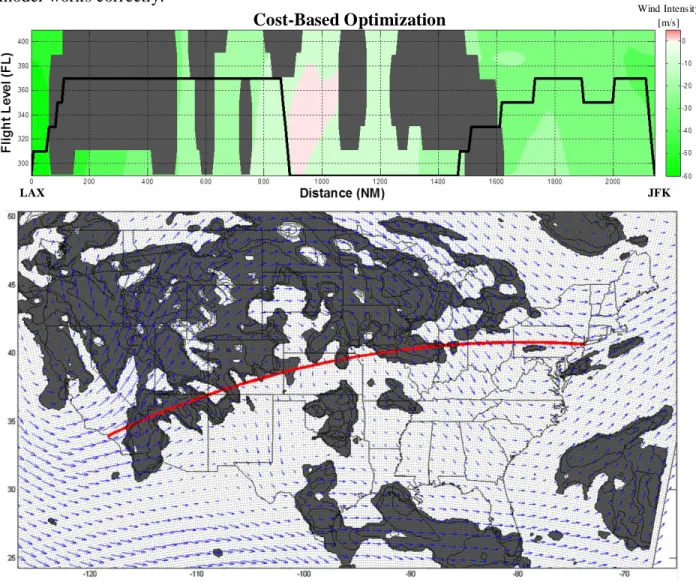
Figure 16 Representative flight profile from LAX to JFK ... 45

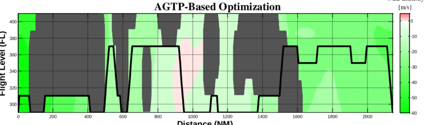
Figure 17 The same representative flight, here using the AGTP-based optimizer ... 46

Figure 18 3-D visualization of the 5 tradeoff variable components using PCA ... 48

Figure 19 Variable correlation using PCA ... 49

Figure 20 Weather days for LAX-JFK for the first day of every month of 2009 ... 52

Figure 21 Example flight profile ... 53

Figure 22 Sensitivity of contrail avoidance to weather conditions ... 54

Figure 23 Contrail production cost tradeoff ... 55

Figure 24 The mean distance of contrail produced ... 56

Figure 25 The rate of contrail avoidance per additional $/NM ... 57

Figure 26 Normalized sensitivity plot ... 59

Figure 27 Cost tradeoff ... 60

Figure 28 Fuelburn tradeoff points ... 61

Figure 29 Representative lateral track types for LAX-JFK ... 65

Figure 30 Vertical AGTP optimization. ... 66

Figure 31 The average net AGTP reduction of various operational strategies ... 66

Figure 32 Comparison between the climate impact reduction and fuel efficiency ... 68

Figure 33 Plot of climate impact and fuel efficiency. ... 69

Figure 34 Sensitivity of AGTP at different contrail RF assumptions ... 70

Figure 35 The energy efficiency . ... 71

Figure 36 Clusters of 2/1/2009 LAX-JFK flight profile solution space ... 78

Figure 37 All flight profiles in the tradeoff solution space ... 78

Figure 38 The reduction of average climate impact ... 79

8

List of Tables

Table 1 NARR-A and RUC 20km ... 35

Table 2 All aircraft types used ordered by MTOW ... 37

Table 3 Climb descent coefficients ... 40

Table 4 Current value structure ... 43

Table 5 The AGTP of fuelburn ... 45

Table 6 Variable component angle from PCA. ... 49

Table 7 Derived price cap for 11 aircraft types... 59

Table 8 The 12 city pairs ... 64

9

Chapter 1 – Introduction

This section motivates the growing climate impact of contrails and the need for mitigation policies to incentivize aircraft operators to fly contrail avoiding trajectories. The objectives of this thesis are to answer the open questions that arise from these motivations.

1.1 Motivation

Contrails, or aviation-induced cirrus clouds, are not traditionally recognized as a major contributor to aviation-induced climate impact as compared to CO2, NOx, and other particulate

emissions. However recent research efforts in Europe have verified the global warming contribution of contrails; one study suggest that contrails and contrail-induced cirrus are the largest single climate impact component from aviation, more than that of CO2 emissions

(Burkhardt & Karcher, 2011). While uncertainty still remains in quantifying the climate impact of contrails, its significance has been suggested across a number of studies. In the latest estimate, climate impact contribution of contrails and contrail-induced cirrus clouds is comparable to that of CO2 and NOx emissions (Figure 1).

10

Figure 1 The latest estimation of aviation radiative forcing (a measure of climate impact) in 2005 by

Sausen et al. The main RF components are CO2, NOx, and contrails (linear and induced cirrus cloudiness). (Sausen, 2005)

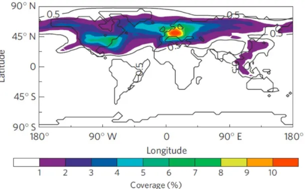
Contrails include linear contrails and the contrail-induced cirrus cloudiness; contrails can grow from the initial line-shaped cloud and spread in coverage given the right weather conditions. In fact, contrail coverage reached up to 8-10% of the airspace in heavy air traffic regions such as the northeast United States and central Europe during the year 2002 (Figure 2). Alongside the growth of the global passenger and freighter jet aircraft fleet, which is projected to double from 2011 to 2031, global contrail coverage will continue to grow unless a mitigation policy such as taxation on contrail production is implemented. Such a policy intends to internalize the social cost of contrails by putting a price on contrail production.

11

Figure 2 Contrail coverage for the year 2002 using a module developed using ECHAM4, an

existing climate model developed by IPCC. The results were successfully verified using satellite observations. (Burkhardt & Karcher, 2011)

Once a policy is established, jet aircraft operators will be incentivized, from a cost perspective, to minimize contrail production during operations. One such contrail minimizing strategy is to operationally avoid contrail producing regions of the airspace by way of cruise phase flight level optimization.

In light of all this, some open questions arise which this thesis will attempt to answer: How, and at what price range, would contrail tax impact cruise operations? And once contrail tax incentivizes operators to fly contrail avoidance strategies, what would be the climate impact of these strategies? There exist other operational strategies that use lateral maneuvering for contrail avoidance, how does the flight level optimization strategy compare? Is one strategy more fuel efficient than the other? Should the optimal strategies be designed for short-term or long-term climate impact? Due to the uncertainty in the current estimate of the climate impact of contrails, how sensitive are the contrail avoidance strategies to different estimates?

12

1.2 Research Goals

This research attempts to accomplish two main goals:

1. Gain an understanding of the impact of contrail tax on the choice of the optimal flight profile and establish a contrail tax price range which contrail avoidance strategy is operationally cost-effective.

2. Evaluate the effectiveness of the flight level optimization strategy in minimizing climate impact.

1.3 Overview

The objectives of this research center on the two main research goals and they are evaluated using two studies: Contrail tax impact study and climate impact study. In order to tackle these objectives, a cruise phase flight level optimization tool was developed to compute contrail avoidance strategies by enabling tradeoffs between contrail production, fuel consumption, flight time, and CO2 and NOx emissions. By adjusting flight levels along the flight

path, the optimal profile is found by minimizing either the total trip cost (in U.S. dollar) or climate impact (in AGTP, a climate impact metric) for the contrail tax impact study and the climate impact study, respectively. From the two main research goals, a number of objectives arise as summarized below:

Contrail Tax Impact Study

 To understand how contrail avoidance may vary based on the weather and aircraft type flown, sensitivity analyses will be done for different weather conditions and different aircraft types.

 To investigates how contrail tax will impact the choice of the optimal flight profile. Using the cost-based optimizer, the optimal profile is found by trading off between the costs of fuel burn, flight time, CO2 emission, NOx emission, and contrail production,

where the cost of contrail production alludes to the contrail tax. This study will determine a price range of contrail taxation at which contrail avoidance strategy is cost-effective.

13 Climate Impact Study

 This study uses the climate impact optimizer to investigate the effectiveness of the flight level optimization strategy in minimizing climate impact. The optimal profile is found by trades off between the climate impact of contrail production and CO2 emission. Since

flight level optimization can be implemented on a variety of different lateral routes such as the great circle route and wind-optimal route, their climate impact will also be examined.

 There are two operational approaches to avoid contrail forming regions: flight level changes and lateral deviations. Complementary to the flight level optimization strategy developed in this research, a research team at NASA Ames has developed a lateral route optimization strategy. The objective is to compare the contrail mitigation and fuel consumption characteristics of both strategies.

 Climate impact is measured at the end of a specific time horizon (i.e. 25, 50, 100 years) therefore the design of the climate impact optimal strategy differs depending on this time horizon. Using the energy efficiency metric, strategies designed for different time horizons are flown and their efficiency are evaluated.

 Due to the uncertainty in estimating the climate impact of contrails, this study uses a range of contrail impact values to evaluate the sensitivity of the results.

15

Chapter 2 - Background

This section discusses the physics behind contrails, along with current best estimates of its climate impact using radiative forcing (RF) as the metric. Using RF as a metric, the climate impact of contrails is compared relative to all known aviation-induced emissions. Once the significance of contrails is establish, the current state of research in contrail avoidance strategies will be summarized. One promising strategy is to operationally avoid contrail forming regions of the airspace by adjust the flight level of the aircraft. To implement this strategy, contrail production will be integrated as an additional constraint in the planning of aircraft cruise operations. The last portion of this chapter will detail the framework by which contrail avoidance is incorporated into the cruise phase route optimization problem.

2.1 The Physics of Contrails

Contrails are clouds of ice particles formed by the condensation of aircraft engine exhaust byproducts such as soot emissions and water vapor, often assisted by the decreased pressure in the ambient air caused by the wingtip vortices (Schrader, 1997). More specifically, the engine exhaust injects water vapor, sulfates, hydrocarbons, and soot particulates into a cold ambient environment where the air is saturated with respect to water, thus forming water droplets that

16

freeze due to the low temperature. These induced cirrus clouds may further persist if the air is supersaturated with respect to ice. Interestingly, natural cirrus formation requires that the ambient air to be of higher ice supersaturation conditions than that of these contrail-induced cirrus clouds. It is thus inferable that there exist cloud-free regions of the airspace where only contrail, not natural, cirrus may form (Burkhardt & Karcher, 2011).

Contrails are the result of the mixing between warm unsaturated engine exhaust gases and cold water-saturated ambient air. The trail of warm exhaust gases drops in temperature and pressure as it approaches ambient conditions. When the ambient air is saturated with respect to water, the water droplets will freeze due to the low temperature. The criterion for saturation with respect to water is met when the relative humidity with respect to water, RHw, is greater than a critical value. The critical relative humidity of the ambient air, rcrit, is a function of the saturation vapor pressure over water, , at a given temperature, T, greater than a critical temperature of contrail formation, Tcrit.

( ) ( ) ( )

Tcrit can be derived and implemented as a constraint in finding contrail producing regions as follows:

( ) ( ) Where

( ), EI is the emission index, CP is the isobaric heat capacity of air, P is the ambient air pressure, ε is the ratio of molecular masses of water and dry air, Q is the specific combustion heat, and η is the average propulsion efficiency of the jet engine (Alduchov & Eskridge, 1996).

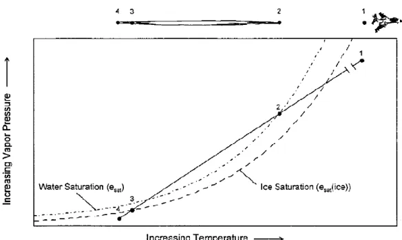
In addition to finding regions with atmospheric conditions that allow contrail formation, the ice cloud may or may not persist depending on the saturation of the ambient air with respect to ice. If the air is not saturated with respect to ice, RHi < 1, the ice crystals will eventually sublimate back into the ambient air as water vapor (Figure 3). Since the humidity (mass of water vapor per unit volume of air, which is proportional to pressure) of the trail of gases is directly

17

proportional to the temperature, the lifetime of the contrail can be depicted as a line against the phase diagram of water.

Figure 3 Non-persistent contrail formation due to the ambient air condition below ice saturation.

From state (3) to (4) of the ice crystals that make up the contrail sublimates back into the ambient air, therefore not persisting (Schrader, 1997).

If the relative humidity with respect to ice, RHi, is greater than 100%, then the contrail will persist for a longer period of time before it sublimates.

Figure 4 Persistent contrail formation occurs when the ambient air is supersaturated with respect

to ice. The phase of the ice crystals that make up the contrail region remain in state (3), thus persists

18

The RHi is found using the ratio between the saturation vapor pressure over water and ice, which has been shown to give results accurate to less than 1% of the standard humidity data (Alduchov & Eskridge, 1996).

( ) ⁄

⁄( )

Contrails not only persist, but also grow. Satellite observations have shown significant increase in cirrus cloud coverage over airspace with heavy air traffic. While contrails are initially line-shaped clouds trailing the aircraft, due to wind-shear they may directly transform into cirrus clouds given favorable meteorological conditions. In fact these clouds have shown lifetimes upwards of 17 hours based on satellite observations and can cover up to ten times the coverage of the initial linear contrail (Sausen, 2005). Contrail formation rates have been measured to upwards of 140 m/min horizontally and 18 m/min vertically (Jager, Freudenthaler, & Homburg, 1998), making them geometrically greater in width than height. Another mechanism by which these anthropogenic clouds may form does not require an initial contrail. The indirect effect of aviation soot emissions on cirrus in the absence of contrails depend on the concentration of and interaction between the emission particles and the ambient air. Essentially, the aerosol injected into the air may act as ice nuclei that seed the formation of cirrus clouds at the right mixing conditions. Albeit there is an inherent uncertainty in distinguishing them from naturally formed cirrus clouds that exist in these satellite observations, thus further meteorological studies are being conducted to refine these results.

The climate impact of contrails is attributed to the radiative trapping of the contrail clouds. In contrast to other emissions such as carbon dioxide gas that mainly absorbs the longwave energy radiating from the Earth’s surface back out into space, contrails has an additional effect of reflecting the downward shortwave energy from the Sun during the daytime, which is commonly known as albedo cooling. Climate impact is measured by quantifying the net energy radiating in and out of the Earth’s atmosphere. The following section will detail one way climate impact can be quantified.

19

2.2 Climate Impact Metric

Before looking at the climate impact of contrails, it is important to first understand the metric used in measuring climate impact. A widely used method of measuring the impact of human and natural factors on climate uses the concept of radiative forcing (RF). Definitively, radiative forcing measures the perturbation of the Earth’s energy budget between two time periods (typically referenced to year 1750, which marks the beginning of the Industrial Era) by finding the net energy difference measured at the tropopause (i.e. FL360 for mid-latitude regions) between the radiative energy from the Sun and the radiated energy from Earth’s surface albedo. RF is measured in the unit of watts per square meter [Wm-2]. The incoming energy the Sun is positive RF and the outgoing energy is designated as negative RF. The RF concept is used to assess the contribution of various environmental factors that affect the radiative balance of Earth; the net positive RF effect of trapping outgoing longwave radiation is commonly known as the greenhouse effect. The standard method of measuring climate impact uses the concept of RF to quantify a metric called global-warming potential (GWP). Most notably used in the international treaty on emissions control known as Kyoto Protocol, GWP is the time integral of the radiative forcing, ΔRF(t), over a region for a specific time interval T0 to T1.

( ) ∫ ( )

Intuitively, this is the net amount of energy trapped by the emission species being measured for a specific time interval. GWP is often used in reports as referenced to an equivalent amount of CO2 needed to generate the same forcing, as is the case for the Kyoto Protocol. This

method of quantifying climate impact is relatively easy to implement; the IPCC First Assessment Report (FAR) described GWP as a “simple approach” for measuring climate impact. However, using GWP also has a few disadvantages (Peters, 2011). Most notably, GWP is a time-integrated measurement that would not distinguish a gas with low RF and long lifetime from another gas with a high RF with a short lifetime. To overcome some of the disadvantages, a novel climate impact metric was developed to take advantage of RF’s approximately linear relationship to the change to the global mean surface temperature. This concept is formally known as the Absolute Global Temperature Change Potential (AGTP):

20

( ) ∫ ( ) ( )

AGTP is found using a convolution integral between the time interval between T0 and T1, where δ(T1-t) is the impulse response function for the surface temperature change at T1 due to a radiative forcing ΔRF(t) applied at time t. The derivation from the RF to the surface temperature change is based on a first-order climate model that assumes exponential decay in the RF. The exponential decay of ΔRF(t) reflects the lifetime of an emissions species via a parameter that captures the heat capacity and climate sensitivity of the gas. Using AGTP, the resulting value is in the unit of kelvin and the decay parameter reflects the residual gas lifetime. Depending on the time horizon, which denotes the time interval from T0 to T1, of interest, the AGTP metric captures the decay characteristic of the RF contributed by each gas. For contrails, the AGTP contribution drops off significantly for longer time horizons. In contrast, CO2 gas are resident in

the upper atmosphere for much longer periods of time and thus their AGTP contribution diminishes less drastically. This behavior is captured in the climate impact study, where contrail avoidance strategies are optimized based on an AGTP-minimal objective function. The AGTP contribution from contrails and CO2 emission are evaluated for a range of time horizons: 25, 50,

and 100 years.

2.3 Climate Impact of Aviation

Before diving into a discussion on the climate impact of contrails, let’s first put climate impact of aviation into perspective. Compared to the total anthropogenic RF, aviation contributed 3.5% in 1992, and is projected to increase to 5% by 2015 (IPCC, 2012). The impact of aviation emission is unlike other types of emission in that the injections are made directly into the upper troposphere and lower stratosphere (at the ozone layer) where they are most potent. The main components of climate impact due to aviation include carbon dioxide (CO2), nitrogen

oxides (NOx), water vapor (H2O), sulphate (SOx), soot, and contrails. Of these emissions, CO2,

NOx, and contrails are the biggest contributors (Figure 1). Unlike CO2 that has a decadal lifespan

allowing for complete mixture into the atmosphere, other gases such as NOx, SOx, and water

vapor (contrail precursor) exist for a shorter period of time and are more concentrated near the flight path where they were injected. Due to these temporal and local characteristics, these gases cause more short-term regional climate responses as opposed to long-term global ones

21

characteristic of CO2.While the impact of common climate impact gases such as CO2 and NOx

are fairly well understood with an established history of assessments followed by policy and taxation proposals, contrails is relatively less understood within the aviation community and have yet to generated enough interest to initiate any efforts to formulate a mitigation policy.

2.4 Climate Impact of Contrails

The RF estimates of linear contrails, excluding contrail-induced cirrus clouds, have varied throughout the years with large uncertainty. Beginning in 1999, the first assessment was conducted by the IPCC on the climate impact of aviation for the years 1992 and 2000 using RF. Recalling that the RF for a particular year represents the energy budget perturbation compared to the 1750 baseline, the RF due to linear contrails in 1992 was modeled to be 20mWm-2 and was projected to increase to 34mWm-2 by 2000 (Figure 5), which signifies a 14mWm-2increase.

Figure 5 Various estimates of the aviation RF for 1992 and 2000 throughout the years by IPCC

and Sausen. Note the variation in the estimate of contrail RF, ranging from 10 to 30 mWm-2. In 2005, a European research effort (2000-2003) published new estimates of the RF for the year 2000 using more refined contrail coverage and microphysical property modeling. The improved estimate cuts the old value by a factor of three to 10mWm-2 (Sausen, 2005). In the

22

latest estimates on the contrail RF of year 2005 found a comparable value of 11.8mWm-2. Therefore although the uncertainty still remains in estimates of contrail RF, independent studies have recently converged on a smaller range of values. Due to the uncertainty in contrail RF estimates, a range of RF values were used in this thesis: 3.3, 10, and 30mWm-2

.

The RF estimates given above focused only on the linear contrails trailing after the aircraft, but neglects the contrail-induced cirrus clouds that appear hours after the contrail formation. The latest research that tries to model the whole life cycle of contrails, including the induced cirrus, suggest that the RF contribution from the subsequent cirrus clouds are almost ten times in coverage than that of the initial linear contrails; albeit the induced cirrus clouds generally have a decayed RF. The conclusion from these studies suggests that the contrails, despite their short lifetime, have a great radiative impact at any one time due to their high RF, resulting in climate impact comparable to that of CO2 emissions (Burkhardt & Karcher, 2011).

An important point to distinguish here is the difference in the lifetimes of contrails and carbon dioxide; assuming all the aircraft in the world are grounded indefinitely, the climate impact due to carbon dioxide will continue to last but the impact of contrails will cease due to their short lifetime. However, at the rate that the air transportation system is currently growing, the impact of contrails will be hard to overlook.

2.5 Contrail Mitigation Policy

As are often done with other climate impact emissions, mitigation policies will likely arise to set limitations on contrail production; it may be requiring jet aircraft operators to internalize the social cost through taxation or setting up a cap and trade system between operating entities, namely airlines. Contrail production, like other greenhouse gas emissions, is a negative externality (unaccounted adverse impact on society) that should be associated with a social cost in the near future if the implications from the recent climate impact studies remain true. A pigouvian tax is a method to internalize the negative externality and is often used for emissions tax. It is foreseeable an implementation of pigouvian tax on contrail production will be placed on airlines, which may be an effective method of mitigate the climate impact of contrail formations. While the social cost per unit (distance or time) of contrail remains to be estimated, it becomes interesting to ask how contrail tax may impact current aircraft operations relative to the current cost structure (current jet fuel price, block hour operating cost, emissions social costs).

23

As such, the implication of the contrail tax impact study is to give a preliminary idea of the marginal operating cost of contrail avoidance. Under the hypothetical scenario such policy creates, aircraft operators will become incentivized to reduce contrail production through mitigation approaches.

2.6 Mitigation Approaches

There are a variety of approaches to minimize contrail production. From a technological standpoint contrail production can be reduced by implementing new engine concepts and aircraft design, alternative fuel and combustion processes, and dedicated prevention devices. Operationally, contrail production can be minimized by using temporal and spatial avoidance strategies.

2.6.1 Technological Approaches

For contrail formation, the mixing process of the engine exhaust with the ambient air is dictated by, among other variables, the engine efficiency. At lower altitudes, more efficient engines cause an increase in contrail producing regions due to their cooler exhaust and more water content. However, at higher altitudes, the difference diminishes (Noppel, 2007). In terms of modifying the microphysics of the exhaust particles, filtration technology during or post combustion can help to reduce the RF of contrails produced. Aircraft design improvements primarily focus on lowering the optimal flight altitude, where contrails are less likely to form. Modification to the wing design may help to minimize wind vortices that assist in exhaust mixing. Fuel-based improvement options such as reducing sulfur content, fuel additives, or fuel alternatives (hydrogen) will lower water vapor output, but at a price of larger exhaust particles that will remain in the atmosphere to seed contrails, albeit lower RF contrails.

Some of these technological approaches are sound in theory. However, recognizing that technological turnover rate of aviation is driven by the rate at which the global fleet evolves via retrofitting and purchasing new aircraft, added with the fact that the average utilization lifetime of an aircraft is on the order of 25 years, the impact of technological advancements is rather slow. Additionally, most of these technological improvements can, at best, suppress the net RF of contrails produced, not eliminating them.

24

2.6.2 Operational Approaches

Operational changes to minimize contrail production take advantage of the temporal and spatial characteristics of contrails. For example, the RF of contrail is higher in the evening since shielding effects during the day reduces daytime RF. During the day contrails are able to deflect short-wave radiative energy from the Sun, thus decreasing the positive RF component. Therefore from a purely contrail minimizing perspective, it would be strategic to limit flights in the evening. To show the shielding effect of contrails during the daytime, the mean net global radiative forcing at the top of the troposphere (12 km or roughly FL390) during daytime has been modeled to be less than that of the full day (R. Meerkotter, 1999). Furthermore, contrail RF has been found to be less during sunrise and sunset (high solar zenith angles) than other times of the day (Myhre & Stordal, 2001), which seem to suggest more flights should be scheduled at dawn and dusk. However, limiting flights to certain times of the day is operationally undesirable given the capacity and economic disadvantages.

Spatially constrained strategies can also be formulated to minimize the net RF impact of the contrail formation. One method is to flying through regions that maximizes the contrail’s radiative shielding component (negative RF) while minimizing trapping reflected radiative energy (positive RF). This method takes advantage of the fact that Earth’s surface has regions of high and low surface albedo (reflectivity). For example, snow-covered regions have high albedo due to high reflectivity of the white surface. Therefore, it is preferable to fly over low albedo regions to minimize the positive RF component. In the extreme case, according to IPCC, scenarios involving cold surfaces, low surface albedo, and high atmospheric humidity may result in net cooling (net negative RF) due to contrails ((IPCC), 1999). Although sound in theory, the unpredictable nature of contrail spreading deems this approach less effective. While the aircraft may strategically fly over low albedo areas, the contrails formed are likely to drift and grow into surrounding areas of higher albedo.

Another approach is to execute flight plans that are designed to minimize flying through contrail producing regions, which can be done by incorporating contrail production as an additional variable to the route optimization problem. Contrail avoidance can be achieved by either lateral deviations or vertical flight level changes, which is the strategy used in this research. While vertical contrail avoidance may require less deviation than lateral, operationally, the

25

additional flight level changes may introduce undesirable complexity in the airspace for the pilot and the controller, not to mention passenger inconvenience. Operational strategies with contrail mitigation have been proposed in the past and route optimization methods have been developed from a number of studies. However, until recently none of the methods considered wind in their simulation environment i.e. (Gierens, 2008) & (Campbell, 2008). By omitting wind effects from the route optimization problem, potential fuel efficient solutions are lost, making the results unrealistic. Recent efforts, mainly conducted by a research group at NASA Ames Research Center, have used actual weather forecast and air traffic data i.e. (Sridhar B. C., 2011) and (Sridhar, 2012). At NASA Ames, the route optimization is done via horizontal maneuvers and does not allow for flight level changes, which is complementary to the approach taken in this thesis. An interesting question to ask is whether lateral or vertical (flight level) optimization is more effective as a contrail avoidance strategy. To answer this question, part of the climate impact study is in collaboration with the NASA Ames research team as the two approaches are compared in terms of their effectiveness in climate impact mitigation and fuel efficiency. The incorporation of contrails to the route optimization problem means increasing the tradeoff dimensions of the flight planning method of current aircraft operations. So before discussing the incorporation of contrail and other environmental objectives into the current flight planning method, the following section will give a background of the method commonly used by airlines today, the cost index (CI).

2.7 Current Operations

In today’s operations, the optimization method that most airlines implement in their flight management computer (FMC) uses the cost index (CI) concept. CI is a parameter that reflects the relative importance between the trip block flight time and the trip fuel consumption.

This index is the ratio of the operating cost (minus fuel) in dollars per block hour and fuelburn cost in cents per pound of fuel. By taking the desirable CI submitted by the operator, the FMC will back out the corresponding performance parameters to calculate the most appropriate

26

speed from climb to descent (Roberson, 2007). To give some intuition on the range of possible CI values for cruise operations, zero results in the most fuel efficient flight plan and maximum CI results in the fastest flight plan. It is clear from this approach that only fuel consumption and operating cost are considered in finding the optimal flight plan, making this a two-dimensional optimization problem. By incorporation environmental objectives such as contrails and other emissions to the function, the dimension of the optimization problem increases to a highly dimensional tradeoff problem. High dimensionality is one of a number of challenges posed by the considering of environmental objectives into the optimization problem.

2.8 Incorporation of Environmental Impact Objectives

To increase the scope of the trajectory optimization problem to include environmental objectives such as contrails, CO2, and NOx, a number of issues must be addressed.

1) Highly dimensional tradeoff problem: The incorporation of CO2, NOx, and contrails

along with the traditional performance objectives of fuel consumption and block operating time calls for an optimization technique capable of handling a tradeoff hyperspace with a large number of possibly intercorrelated objective variables.

2) Multiple metrics: The traditional performance objectives are typically measured in dollar cost per gallon of fuel or block operating hour. On the other hand, environmental objectives are measured by climate impact metrics such as AGTP. Therefore the joint optimization problem must be capable of cross-metric evaluations that make intuitive sense.

3) Multiple stakeholders: Typical of most air transportation system design and optimization problems, the cruise operations problem is of interest to a number of different stakeholders in the aviation community. The airlines are interested in cost efficiency and customer satisfaction, the air traffic control towers are interested in safety, capacity, and workload, and the environment interest groups are interested in climate impact of aviation.

In light of these requirements inherent to the optimization problem, this study looks to utilize a suitable tradeoff framework that has been developed previously for these purposes.

27

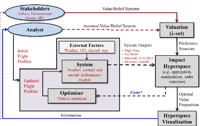
2.9 Tradeoff Analysis Framework

The framework was designed for the purpose of analyzing tradeoff hyperspaces often seeing in the design and operations of systems that consider a high number of tradeoff variables (O'Neill & Hansman, 2012). The robustness of the framework allows it to handle a wide range of highly dimensional tradeoff problems that exist in the air transportation system, making it appropriate for the cruise operations optimization that considers 5 variables: fuelburn and flight time incorporated with the environmental objectives CO2, NOx, and contrails. The framework

allows for analysis and visualization of highly dimensional system outputs, Y, as shown in Figure 6. Apart from a baseline framework, there exists a version of the framework that is adapted for systems with multiple stakeholders and with internal optimization. This study utilized this version of the framework with optimization.

Figure 6 Tradeoff framework with optimization for multiple stakeholders.

In this approach the user of the tradeoff framework is an analyst, such as a researcher interested in the tradeoff problem. The analyst makes proposed changes to a system model, which describes and represents the system of interest. This model is further contextualized to the tradeoff problem with external factors, which creates a full simulation environment to generate

28

the system outputs, ⃗ . In the cruise operations optimization problem, the system outputs are fuelburn, flight time, CO2, NOx, and contrails. The analyst also has an assumed value and belief

system for the tradeoff objectives that can be formalized into a set of valuations, called a preference structure. The preference structure is the value of cost the analyst places on the tradeoff variables. The system output and the preference structure are aggregated to form the tradeoff space termed impact hyperspace. In this space, the system outputs are presented reflective of the assumed value the analyst imposed on each tradeoff objective. With further exploratory data analysis such as dimension reduction, an otherwise hyperdimensional tradeoff space may be visualized. Such hyperspace visualization allows the analyst to obtain the necessary information for decisions on proposed changes and assumed value and belief system, thus completing the closed-loop framework.

The tradeoff framework used in this research also has an optimizer for finding the most valuable proposed change given a set of valuation. Under this framework, the analyst is no longer responsible for determining the proposed changes. Instead, the analyst inputs the necessary initial condition the optimization algorithm needs to find the optimal proposed changes. Note that for the case of multiple stakeholders each with their own set of valuations, a wide variety of approaches can be taken such as combining the valuation sets together into a weighted average set reflecting the influence of each stakeholder to the system of interest.

2.9.1 Valuation (λ-set)

The tradeoff framework considers multiple stakeholders, each with their own respective value and belief system. Each individual stakeholder’s preference is reflected in the valuation component of the framework. The weighting, or cost, a stakeholder places on every variable is referred to as the λ of the variable, which makes the group of valuation for a particular stakeholder the set of λ, or λ-set. The analyst may choose to input a number of assumed value structures reflective of the different stakeholders with interest in the system for an exploratory purpose.

The purpose of the valuation is to reflect the stakeholder’s preference structure. The approach taken in this research has the objective function, V, as a linear combination of the individual stakeholder’s variable cost, λi, and the system output, Yi.

29 ∑

Therefore, depending on the weighting of preference structure on each tradeoff variable, the resulting objective function cost will reflect the relative importance the stakeholder places on each variable. The valuation becomes important in this research since there are two fundamentally different objective questions it is trying to answer. To do so, two valuations are used in this research to reflect two different stakeholders. For the contrail tax i mpact study, the stakeholders are the cost-driven players in aviation such as airlines and other aircraft operators. For them, the most important objective is to maintain cost-optimal operations. Therefore, as suggested by the cost index concept introduced in Chapter 1, the most important tradeoff variables currently are fuel burn and flight time. Fuel burn incurs fuel cost that has risen substantially in recent years. Flight time relates to block operating time that includes crew, maintenance, and aircraft cost. The objective of this research is to incorporate environmental costs to the traditional operation tradeoffs, with the research focus on contrails. This can be accomplished by adding the emissions and contrail cost to the valuation.

On the other hand, for environmental interest groups such as the Intergovernmental Panel on Climate Change (IPCC) whose authority on policymaking is based on climate impact assessments, the valuation changes to reflect the importance of the climate impact of emissions and contrail production. In order to measure the climate impact of operations, dollar cost is no longer sufficient and instead AGTP is used. The valuation in this study maps the system model outputs into the impact hyperspace as AGTP measurements that quantify climate impact as a global temperature change.

31

Chapter 3 - Methodology

The cruise phase flight level optimization tool developed in this research uses the tradeoff framework with optimization to incorporate contrails and emissions as additional variables to the traditional route optimization method that trades between fuel consumption and flight time. This section details the various components of the tool such as the system model and the optimizer. There are two versions of the system model used to conduct analysis for the two main studies: contrail tax impact study and climate impact study. While the two versions are similar in most aspects, there are some differences in the data sources and the calculating of the optimal profile that will be detailed in this section. Before the two studies are presented, a preliminary study using principle component analysis (PCA) is presented to illustrate how the fuelburn, flight time, and emissions correlate with contrail production.

3.1 Tradeoff Framework with Optimization

To implement the tradeoff framework to the cruise phase optimization problem, the first step is to construct a robust modeling environment that accurately reflects the cruise phase of flight. The modeling should be able to fly a mission and produce the desired outputs, namely fuel

32

consumption, time of flight, CO2 and NOx emissions, and distance through contrail regions, of

typical missions with high fidelity (Figure 7).

Figure 7 Tradeoff framework with optimization contextualized to the cost-based version of the

cruise phase altitude optimization problem. *denotes where the metric changes from dollar cost to AGTP for the AGTP-based version.

With five tradeoff variables to consider, this optimization problem is computational complex, which makes parsing for the full output solution space computationally infeasible. Instead, only the optimal solution space is parsed using the tradeoff framework with optimization. By approaching the cruise optimization as a graph search problem where the nodes are transition points to remain level, climb, or descent and the arcs are the incremental path along the flight, the vertical optimizer developed for this study uses an iterative shortest path heuristic that finds the cost-minimal flight profile. In order to achieve the different objectives set out in this research, the cruise phase altitude optimization problem was approached using two sets of valuations (λ-set) reflecting two different stakeholder perspectives. The λ-sets are the distinguishing factor between the cost-based and AGTP-based versions.

33

3.2 Data Sources

The system model integrates a variety of data sources for weather, contrail, and aircraft modeling. The goal is to create a realistic physics-based modeling environment that can generate accurate outputs for cost and climate impact analysis.

3.2.1 Weather Data

To fully model the cruise operations, it is important to account for the ambient temperature, pressure altitude, and wind along the flight path in determining the groundspeed of the aircraft. Furthermore, ambient temperature and relative humidity are needed in modeling the contrail formation regions of the airspace. The necessary weather information is gathered from two forms of weather data provided by the National Oceanic and Atmospheric Administration (NOAA).

In the contrail tax study, the weather data used was the North American Regional Reanalysis-A (NARR-A). NARR-A is a re-analysis data product from the web-accessible National Operational Model Archive and Distribution System (NOMADS) data archive. The data are generated by assimilating observations and satellite data of the past atmospheric conditions of North American region. It is the most accurate source of historic data with information on temperatures, winds, pressure, and humidity, amongst other things. Re-analysis data such as NARR-A is most appropriate for the purpose of this study of modeling historic weather days.

34

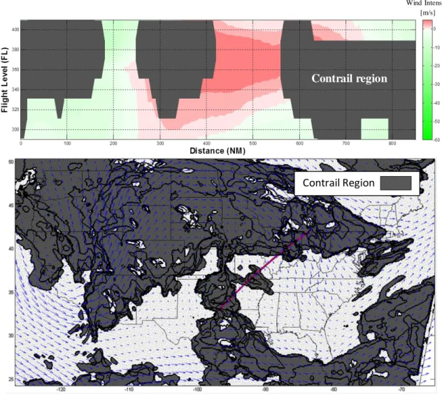
Figure 8 Representative weather using RUC data: Wind optimal DFW-DTW on a B733 for

April 10, 2012 at 16UTC. The top plot is the vertical profile of the flight showing the wind intensity (green & red) and contrail forming regions (gray). The bottom plot shows the map view of the flight with the wind vectors shown as quivers and the contrail forming regions ( gray) stacked from FL280 to FL440.

In the climate impact study, where the environmental impact of contrails was evaluated, the data came from NOAA’s weather prediction model called Rapid Update Cycle (RUC) as shown in Figure 8. RUC data are mainly used when the weather forecasts are of interest, which is not the case for this study. RUC was used in an effort to conform to the data source of our collaborators at NASA Ames for the sake of comparison; they have developed a lateral optimizer for cruise operations complementary to our vertical optimizer. Since the forecasting feature was not used, only the RUC initial conditions were parsed for weather modeling. In regards to the

Wind Intensity [m/s]

Contrail Region Contrail region

35

disparities between the two data sources, aside from negligible temporal and spatial resolution differences, the outputs are similar (Table 1).

Table 1 Notable differences between the data parsed from NARR-A and RUC 20km.

NARR-A RUC 20km

Spatial Resolution 32 km X 29 pressure levels 20 km X 37 pressure levels

Temporal Resolution 3 hour updates 1 hour updates

Years available 1979 - 2012 2002 - 2013

The file format of both weather data types is Gridded Binary (GRIB), a standard for meteorological data and has two generational versions, GRIB and GRIB2. The map grid of the weather data is of the North American region and is projected using lambert conformal conic, which is preferred in gridding middle latitude regions for its accurate portrayal of distance and spacing. Aeronautical charts typically use this type of projection; i.e. a straight line on a lambert conformal conic map is a great circle track. The interpolation of the weather data from the data grid along the flight track is a nearest neighbor approach as shown in Figure 9. For example, the weather data used to generate the wind in the top plot of Figure 8 is interpolated from the lateral track for FL290 to FL410 (8 of the 37 pressure level data layers) shown in the lower plot.

3.2.2 Contrail modeling:

The persistent contrail modeling for the operating cost portion of this study applied the RHw and RHi criterions, which is an adequately modeling approach when compared to satellite

observations (Degrand & Carleton, 1977-1979). However, this simplification it does not capture contrail dispersion that occurs under realistic atmospheric conditions. Recent advancements in contrail modeling have been able to incorporate Lagrangian particle dispersion model and cloud microphysics model to capture this spreading effect. NASA Ames, the author’s collaborators on a portion of the climate impact study, extended the simplified persistent contrail model to include this dispersion modeling and provided us with the contrail data for analysis in the climate impact study. The contrail regions generated for Figure 8 and Figure 9 used this contrail model.

36

Figure 9 Airspace over Missouri and Illinois, mid-cruise for the DFW-DTW flight showing the

map grid with the lateral track and contrail region for FL390. The wind vectors are shown in quivers. The circled points are the closest data points to the track from which the weather data is interpolated and used to generate the vertical weather profile depicted in the top of Figure 8.

3.2.3 Aircraft performance modeling:

Another aspect of the cruise operations that requires modeling is the aircraft performance characteristics. The fuel burn is very dependent on the aircraft type, as are the operating time and emissions. The tool used in this study is Project Interactive Analysis and Optimization (Piano-X) developed by Lissys. This professional aircraft analysis tool has a wealthy inventory of existing aircraft types along with high-fidelity aerodynamic and performance data for each aircraft.

Using Piano-X, aircraft performance data are exported as lookup matrices with dimensions of gross weight (ranging from operating empty weight to maximum takeoff weight), altitude (FL290 to FL410), and Mach number (minimum and maximum allowable per aircraft). The performance variables of interest to the analysis include the specific air range (SAR) and NOx emissions index. SAR, the distance traveled per unit of fuel used, makes a direct

relationship between the fuel consumption with the distance traveled. By using wind-corrected distance flown, the fuel consumption can be integrated. The SAR value extracted from Piano-X uses values assuming default cruise condition.

37

To find the NOx emissions output, the emissions index is extracted from Piano-X. This

index defines the grams of NOx produced per kilogram of fuel used. Based on the flight

condition, Piano-X uses the Boeing fuel flow method 2 (Boeing 2) to calculate the emissions index relative to a reference index value from the ICAO databank. Boeing 2 is an emissions estimation method that uses non-proprietary engine emissions characterization to approximate emissions to within 10 to 15% of estimates generated from proprietary modeling, which are superior due to higher quality of data. Note that CO2 emission is directly proportional to fuel

burn; 1 kg of jet fuel produces 3.16 kg of CO2.

A total of 11 aircraft types were used in this research. Their lookup matrices were generated from Piano-X and used in the aircraft performance model integrated in the system model (Table 2).

Table 2 All aircraft types used ordered by MTOW. The preliminary and contrail tax studies used

all of the aircraft, whereas the climate impact study used the aircraft types shaded in green.

B737-300 B737-700 B737-800 MD83 A319 A320 B757-200 B767-200ER B767-300ER A330-200 B777-300ER Seating Capacity 150 215 215 172 156 180 239 255 350 380 550 Length (m) 33.4 42 42 45 34 38 47 48.5 55 59 74 Wingspan (m) 28.9 36 36 32.8 34 34 38 47.6 48 60 65 Operating Empty Weight (lbs) 72100 74000 74000 79700 90000 107000 128000 181610 198000 264000 370000 MTOW (lbs) 138500 150000 150000 160000 166000 170000 255000 395000 412000 520000 775000 Cruise Mach 0.74 0.74 0.74 0.76 0.78 0.78 0.8 0.8 0.8 0.82 0.84 Max Range (NM) 2300 2400 2400 2500 3600 3200 3900 6385 6000 7250 8000 Operating Cost* ($/BLK hr) 1900 1700 2000 2000 1900 2000 2500 2800 3300 2900 4000

38

3.3 System model

Figure 10 The system model of the tradeoff framework with optimization adapted to the cruise

problem encompasses the external factors, the various models, and the optimizer. * The contrail RF assumption only applies to the climate impact version of the system model.

Weather, contrail, and aircraft modeling create the simulation environment for the cruise phase of flight, with robustness to handle a variety of weather conditions, O -D pairs, and aircraft types. The system model, shown in Figure 10, integrates this environment with a shortest path heuristic in a closed loop feedback to optimize these missions. The external factors specify the lateral track and weather day of interest, the system model extracts the along-track wind vector, temperature, and relative humidity for every pressure altitude that is available for flight level change from the NARR-A/RUC database described in the previous section. Based on the type of aircraft specified to fly the particular mission, the aircraft performance characteristics throughout the cruise mission can be obtained from the lookup table generated from Piano-X. The cruise operation modeled in this study is discretized by the number of flight level changes (2000 ft. increments) and along-track transitions points dictated by the distance traversed by the aircraft climbing or descending to an adjacent flight level. This suggests that the flight level optimization problem could be approached as a shortest path problem with a graph network of transition points where the aircraft has the choice of ascending, descending, or maintaining level cruise. The heuristic used is a k-shortest path (KSP) algorithm based on Dijkstra’s graph search method. Due to the weight-dependent nature of aircraft performance, interim flight profiles found by the algorithm were automatically flown iteratively until the weight profile converges to a final optimal flight profile. The optimal profile is found by evaluating the cost by applying a cost

39

structure to the system outputs of fuel burn, operating time, CO2, NOx, and contrail produced

until a minimum cost is found.

For the contrail tax study, the cost structure, or λ-set, uses the most current fuel (λfb),

block operating ( λoc), and emissions and contrail social costs (λco2, λnox, λcont) in dollar per unit

output. In the climate impact study, the λ-set consists of only λfb and λcont in AGTP unit of kelvin

of temperature change per unit output. The outputs are evaluated in the impact hyperspace where the tradeoff solution space is generated by the system model.

3.3.1 Defining the Cruise Profile

The cruise profile for flight level optimization can be constructed into a directed graph from origin (start node) to destination (end node). For a directed graph G(N,A), the nodes, N, are all the possible altitude change points along the flight profile and the arcs, A, joining the nodes are incremental paths along the flight with costs associated with them. The arc costs are based on the linear combination of the individual outputs with their perspective valuation, normalized to the distance of the incremental path.

Figure 11 Visualization of the graph network of a cruise profile. Each node, N, is the aircraft’s

transition point to climb, descent, or remain level. The arc is associated with the incremental path distance it takes for the aircraft to climb to the next flight level (+200ft).

40

The distance of the incremental paths is variable to the assumed average climb rate of the aircraft. Based on the climb rate, the incremental path distance is the distance the aircraft traverses to climb to the next flight level (+2000 ft.). For the case of an A320, the path distance is roughly 7.5 nautical miles. Therefore, here we made the simplifying assumption that the descent distance is the same as the climb distance. In real life, typically descent rates are faster than climb rates, as the operator often want to maximize the fuel efficiency of the higher altitude before dropping to a lower flight level. Furthermore, the climb and descent aircraft performance characteristics are assumed to be a coefficient factor of that of level cruise. Based on a previous study, these coefficient factors were shown to match Piano-X calculations with good accuracy.

Table 3 Cruise phase climb and descent coefficients (unitless) used to estimate non-level flight

performance characteristics

Climb Descent

Fuel burn & CO2 1.215 .79

Flight time 1.003 .998

NOx 1.43 .66

3.3.2 Vertical Optimizer Heuristic

The first criterion for the choice of heuristic used is efficiency. The algorithm that comes to mind is Dijkstra’s graph search algorithm, mainly for its relative ease in implementation and its wide use in analogous shortest path problems. Another criterion considered in the choice of heuristic is the capability of finding more than one optimal solution. The need for multiple top solutions roots from the highly constrained nature of cruise operations in real life; i.e. limitation on the number of altitude changes from the air traffic controls or avoidance of heavy traffic altitudes over an airspace region, to name a few. Without explicitly considering for each constraint, the heuristic should be able to recommend a number of top solutions for the operator to choose from as an advisory tool, allowing the operator to decide based on the constraints of each scenario. Most single shortest path algorithms such as A* grow exponentially in computation time with each additional solution, making them rather cumbersome to run if more than one solution is desired. Therefore to satisfy the second criterion, the system model uses the k-shortest path (KSP) algorithm (Yen, 1971). This algorithm is specifically designed for finding k number of solutions without sacrificing computation time with additional solutions. In fact, the computation time grows linearly with increase in k (Figure 12).

41

Figure 12 The runtime of each additional solution using KSP grows linearly as opposed to the

exponential growth of single solution graph search methods.

3.3.3 Weight Convergence

Since the aircraft performance characteristics are dependent on the weight of the aircraft, a feedback loop is needed to ensure convergence of the gross weight profile. This is due to the path-dependency of the gross weight; depending on the flight profile taken to get to a point along the flight, the gross weight of the aircraft and subsequently its performance characteristics changes. The goal is to iteratively fly the optimal profile found by the heuristic for convergence to a realistic weight profile. The initial gross weight profile inputted into the optimizer is that of a worst-case scenario 1800NM mission at maximum allowable Mach speed and FL290 flown in Piano-X. Since 1800NM is longer than most missions flown for this study, the top of climb (TOC) weight for the initial gross weight profile is in general an over-estimation for other missions used in this study, making it a bad reference weight for convergence. Instead, the top of descent (TOD) weight at the end of the worst-case scenario flown in Piano-X is use. This weight is not as dependent on the trip length and provides a better reference weight for convergence. The approach of this iterative step is as follows:

Step 1: Find the interim optimal cruise profile using an initial aircraft gross TOC weight from Piano-X, which simulated a worst-case 1800NM mission profile at maximum allowable Mach speed and FL290.

0 5 10 15 20 25 30 35 40 45 50 0 100 200 300 400 500 R u n T im e ( S e c o n d s ) Number of Solutions, k

42

Step 2: Then fly the profile to obtain the total fuel burn weight from the first profile. Step 3: Add this total weight of fuel burn to the TOD weight from Piano-X, creating a new top of cruise weight more suitable for the mission. Note that this total fuel burn weight is found using the over-estimated TOC weight, therefore the new ‘lighter’ weight profile will, at most, burn the same amount of fuel. Find the new interim optimal cruise profile using the new TOC weight.

Step 4: Iterate steps 2 and 3 while keeping track of the change in the weight profiles until the weight profile of the optimal solution converges.

3.4 Study-specific System Models

There are two versions of the system model used in this research, specific to the two main studies: Contrail tax impact study and climate impact study. The framework remains the same for both versions. The distinctions lie in the valuation (λ-set) to reflect the different perspectives of the two studies, plus the weather and contrail model used.

3.4.1 Cost-based Optimization

In the cost-based version, the system model is designed for the contrail tax impact study to optimize based on an operating cost based objective function (Figure 13). That is, every tradeoff variable is valued in dollar cost. The intent is to explore the various cost-based tradeoffs associated with contrail avoidance; namely, the total operating cost and additional fuel cost tradeoffs.

Figure 13 The cost-based system model used in the contrail tax studies. The distinctions from

the climate impact portion lie in the λ-set, the resulting network graph, and weather and contrail modeling (shaded).

43

The λ-set used in the cost-based system model comes from the latest estimates of jet fuel price from International Air Transportation Association (IATA), block operating cost for specific aircraft type, social cost of CO2 from the U.S. Environmental Protection Agency and NOx from

the Department of Energy (Table 4). There is no current estimate on the social cost of contrails.

Table 4 The latest estimates of variable costs make up the λ-set used in determining the

operating cost of contrail avoidance.

λfb λoc λCO2 λNOx λcontrail

Jet Fuel Cost Block Operating Cost Social Cost of Emissions

3.00 $/gal i.e. A320: 2000 $/Bhr 0.023 $/kg 4.05 $/kg ? $/NM

IATA 2012 Aviation Week AOC & S SCC from US EPA DoE estimate

The weather model used in the cost-base system model is the NARR-A reanalysis data from NOAA. The contrail model is based on the relative humidity criterions discussed in detail in Chapter 1. The arc cost calculated in the network graph is a linear combination of the λ-set and the outputs of all five tradeoff variables. In the contrail tax study, the cost-based system model is used to analyze the impact of different cost of contrails on the optimal flight profile.

3.4.2 AGTP-based optimization

For the climate impact study, instead of the dollar cost metric used in the cost-based version, the AGTP-based system model is used to generate optimal profiles that are evaluated in terms of AGTP, a climate impact metric that measures the instantaneous change in the global temperature due to a radiative forcing (RF). The AGTP-based system model is used to tradeoff between the benefit of contrail avoidance and the negative impact of CO2 emissions measured at