High-Performance Computing for Data Analytics
Dimitri Perrin, Marija Bezbradica, Martin Crane, Heather J. Ruskin Centre for Scientific Computing & Complex Systems Modelling
Dublin City University Dublin, Ireland
Email:{dperrin, mbezbradica}@computing.dcu.ie
Christophe Duhamel ICD-LOSI, STMR (UMR CNRS 6279)
Universit´e de Technologie de Troyes Troyes, France
Email: [email protected]
Abstract
One of the main challenges in data analytics is that discovering structures and patterns in complex datasets is a computer-intensive task. Recent advances in high-performance computing provide part of the solution. Multicore systems are now more affordable and more accessible. In this paper, we investigate how this can be used to develop more advanced methods for data analytics. We focus on two specific areas: model-driven analysis and data mining using optimisation techniques.
1. Introduction
Advances in high-performance computing (HPC) have resulted not only in improved performance but also in greater availability of such resources. The cost per GFLOPS dropped below $1000 for the first time in 2000, below $42 in 2009 [1], and below $2 in 2011 [2]. Ongoing development of cloud-based solutions is likely to further increase availability and affordability.
Such resources are particularly needed in data analytics, where finding hidden structures and patterns in large heterogenous datasets is typically computer-intensive.
In this paper, we consider two fields of data analytics where HPC availability is already having a significant impact, namely analysis based on optimisation techniques and model-driven analysis.
For each approach, we provide an overview of the challenges and detail how high-performance computing can be used to solve these. Two case studies are detailed: pharmaceutical R&D and genetic research.
2. Data analytics in pharmaceutical R&D
The use of data analytics in drug development and discovery was historically used in limited scope as the process of in vitro drug release was considered akin to a black box, where different inputs were varied in order to tailor desired outputs. In this sense, internal dynamics of the pharmaceutical device could not be understood solely
by pure observation as these presents a superposed picture of the phenomena involved.
Using pharmacokinetic modelling from the drug discovery phase through to development and manufacturing can provide: (i) support for the decision making process, (ii) improved and effective usage of drug development time with reduction of design parameter space, and (iii) the basis for analyses both within and between input data sets.
This reduces the amount in vitro / in vivo testing required, important to cost-effective and flexible solutions. Hence, in
silico modelling and analysis enable extensive offline testing
and evaluation of parameter sensitivity [3].
2.1. Advantages of probabilistic modelling
Drug dissolution system (DDS) models can be broadly split into two categories. Mechanistic models attempt to describe the system precisely, using sets of differential equations, which are useful for data analysis purposes only if relevant input parameter values, often unobtainable through in vitro testing, are known. As an alternative to these, probabilistic models, requiring less detailed initial knowledge of dissolution parameters are applicable to a wider range of systems, making these more practical in enterprise applications. Combined with Cellular Automata (CA) methods a bottom-up approach is employed to predict global drug behaviour by describing individual polymer interactions using a combination of physico-chemicals laws (such as Fick’s) and probabilistic distributions. Initial cell states are randomised using Monte Carlo algorithms, replacing the need to precisely define the initial set up, apart from giving the outline drug device structure. Following the first use of CA in pharmaceutical modelling [4], many subsequent models have been described in the literature [5]–[8].
2.2. Advantages of high performance computing
In general, there are two sources of large data in pharmaceutical analysis. The first is due to novel drug formulations having a considerable amount of experimental data from the design stage which require processing in order 2012 IEEE/ACM 16th International Symposium on Distributed Simulation and Real Time Applications
to deduce relations between design parameters. Synthetic sources depend on the device where fine resolutions is needed for micro- and nano- scale simulations. These require high performance, large scale infrastructure to execute. Even though such resources today are readily available, either from local scientific computing clusters or commodity public cloud infrastructure, the algorithmic solutions in these applications are not reported in the scientific literature [3]. Furthermore, in parallelisation of cellular automata systems, the key challenge to be solved is that of efficient transfer of cell states across process boundaries where communication is expensive [9]. This problem becomes more complex for multiple scales as we switch from classical CA models, to ones incorporating agent-like behaviours, such as those of particle diffusion within the drug device.
In this paper we present a high-performance probabilistic CA framework for large scale data processing, developed in collaboration with a pharmaceutical enterprise partner, Sigmoid Pharma Ltd. The framework is used for prediction of drug release rates from pharmaceutical devices used in
controlled drug delivery, which aims to deliver specific
dosage profiles and reduction of negative side effects, such as dose dumping. Controlled drug release may be achieved in many ways, such as by coating the active ingredient (drug) using one or more layers of polymeric coatings, which are designed to protect the core component as it traverses the upper intestine and enters the gastro-intestinal (GI) tract.
The main advantage of using a generic CA framework is its adaptability to different model scenarios in terms of supporting various geometries (such as 2D, 3D, tablets, cylinders and spheres), as well as incorporating a range of complex phenomena, from basic release mechanisms (such as diffusion and erosion) to analysis of more specialised ones (such as clustering of drug in coating or influence of the dissolution environment).
In Section 2.3 of this paper, we present the data analytics workflow used for pharmaceutical data collection, processing, modelling and analysis. Section 2.4 introduces the CA framework developed and demonstrates a referent model, as well as covering the main HPC algorithms used for model parallelisation and optimisation. Analyses for the simulations are discussed in Section 2.5. Finally, in Section 4 we outline the main findings and possible future directions for model development.
2.3. Data analysis workflow
In vitro and in silico data analysis and development of
the relevant model were performed based on the workflow presented in Figure 1 [10]. This continuous feedback loop is composed of several distinct stages, separated into two main parts (enterprise and modeller).
Initial drug design and in vitro testing in the USP apparata [11], is performed by the enterprise partner. The data are
Figure 1. Data analysis and modelling workflow
filtered to determine the variables of interest, intrinsic to the drug device design process (input parameters such as geometry, size, drug loadings, and coating thicknesses) and relevant to the modeller (e.g. types of physical processes/chemical reactions present, release curves for different parameter sets, etc.). The data obtained are used to construct a CA model describing different assumptions about the dissolution processes present.
The models are then optimised for parallel execution and simulated on high performance computing clusters for various input data sets, in order to maximise the gain from running many simulations at once. As the laboratory testing is performed for periods of up to 24 hours, then in order for
in silico simulations to be cost-effective, the workflow and
the underlying framework must be able to support running large numbers of simulations over a relatively short time.
Two main sets of simulation results are generated: (i) a control set, which validates results against the known experimental data points and is used to asses model usability for predictive purposes. For controlled release, a sigmoidal (”S” Shaped) release curve is expected, demonstrating properties of a zero-order release kinetics during a period when the device passes through a region of maximum adsorption; (ii) a generic data set showing variations of release profiles, dependent on parameter changes, which can then be used to feed back into the drug design process.
If model validation is promising, extensive optimisations can also be performed in order to ensure model robustness and reusability for similar drug device analysis.
Insight on system evolution is also provided by graphical representation of the model, which captures successive
stages of the dissolution.
2.4. Analytical framework
The developed framework was used to build several models (for single [12], and multi-layer coated spheres) that define a set of common key states and transition rules describing physico-chemical phenomena of interest. Each cell state includes information on the type, (i.e. solvent, core, coating, drug and pore), with state transitions and drug movement simulating three phenomena of interest: (i) degradation of polymer chains; (ii) expansion potential of polymer chains; (iii) number of drug particles present in the cell.
Degradation (erosion) of polymer chains into oligomers and monomers depends on the information known about different polymer properties. This rule can occur at a fixed rate, using a set probability [8], or follow a probabilistic distribution (e.g. Erlang [5]), to allow for degraded cell transitions to a solvent state. Polymer expansion (swelling) occurs using an analogous mechanism, instead of a cell transitioning into a new state; it replicates itself into a neighbouring cell. The penetration of solvent inside the cells allows free diffusion of drug molecules.
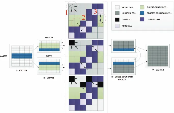
Each rule can be simulated independently and in parallel. An example for this simulation using parallelisation can be seen from Figure 2. Phenomena are simulated using a sequential CA approach, with all cells in the matrix being updated once every iteration, depending on their previous state and that of their neighbours.
Depending on the available infrastructure and on the need for model fine resolutions, the framework is adapted for different parallelisation strategies [9]. Process level parallelism, which would require more extensive computing resources, can be used at the development and analysis stages where there is a need for processing of large data sets of experimental data, in order to narrow the window of input for the wet-lab experiments. Lighter, thread level parallelism can be utilised even in laboratory conditions and is adequate for further analysis of single parameter ranges.
The framework adopts a hybrid approach, allowing selection between the two strategies, which maximises the utilisation of available high performance infrastructure by applying both thread and process level parallelism. Inter-thread and inter-process communication overhead occurs as a consequence of the cell state being exchanged during execution rule and is solved by introducing boundary cell layers, where communication is either sequentialised (i.e. using locking) for the case of threads, or delegated to one of the two neighbouring processes for process level.
Figure 2 shows the separation of model space into individual sections that can be simulated independently on any number of execution nodes. The separation, and subsequent collection of simulated results follows
a “scatter-gather” pattern. One, master process spreads (scatters) the workload across all the nodes, and, after the processing is finished, it collects (gathers) the results back. The analysis and extraction of output data follows and is recorded for the current iteration. The simulation cycle then starts over.
The central part of Figure 2 shows the described CA rule execution in the context of the hybrid model. The top panel of the diagram represents the diffusion process through three distinct update scenarios. In scenario 1, we have the normal, isolated (i.e. independent of shared space), rule execution, where a set of drug molecules can choose to move to a suitable neighbour. Scenarios 2 and 3 display rule updates which occur inside the shared layer. In this case state locking is performed, and cell access is sequentialised on a first-come first-served basis. In scenario 2, there is no additional contest from the other thread, so regular cell state update occurs. However, in scenario 3, as the synchronous CA update mechanism is used, a second update will not be aware of the changes made by the first, resulting in a need to resolve the conflict. In this case, we assume the resulting state will be cumulative and both diffusions are permitted, unless a super-saturation of the cell occurs.
The middle panel in the diagram in Figure 2 shows similar update scenarios in the context of erosion rules. As rules in this case are passive and affect the self-state only, there is less potential for conflicts. In case of shared layer access, however, it is still necessary to lock the cell, in order to prevent other rule types from affecting it.
Finally, the bottom panel of Figure 2 represents the scenarios for simulation, incorporating swelling. These are fairly similar to the diffusion updates, with further complexity that polymer transfer to neighbouring cell occurs, influencing erosion cycle in the subsequent iteration. It is also important to note, that conflicts can occur in shared cell updates of different types (i.e. swelling and diffusion or erosion and swelling). In this case, we define an allowed order of cell updates, where a state change will block further updates of certain kinds. For example, an erosion of a cell which degrades the entire remaining polymer will further block any swelling rules which can be executed from that cell.
2.5. Results
Figure 3 shows the parallelisation efficiency of the model presented for different number of cores. As expected, for fine-grained problems, a hybrid solution has the advantage over individual thread-level and process-level solutions. The utilisation of the available processing power is highest for low-core counts, where inter-process communication does not occur (1 to 12 cores). For extended range, utilisation falls somewhat artificially due to a data load factor. The utilisation on the higher core number is thus low, as simulations were
Figure 2. Hybrid parallel model with main rule types
Figure 3. Hybrid parallelisation efficiency
performed for data sets of millimetre scale, while at the lower scale efficiency is higher as larger workloads are assigned to each core [13].
An example of typical data analysis performed on model input parameters is shown in Figure 4 [12]. The effect of degradation rate of the chosen polymeric coating on resulting drug release curve, from a single-coated sphere,
Figure 4. Analysis of coating degradation rate influence on drug release
was investigated. The effect of coating degradation in range over 1 to 10 days was simulated. The slower degradation causes decrease in porosity resulting in slower overall drug release [12].
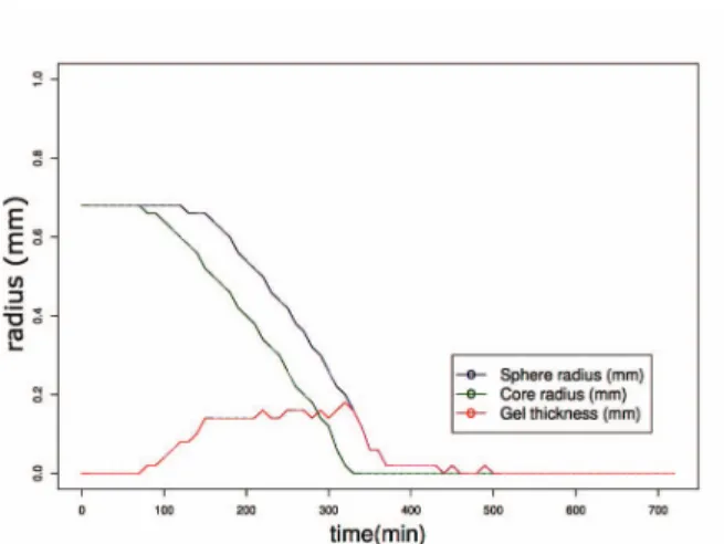
When analysing superposed phenomena, common in controlled release, the dynamics of device radii are
Figure 5. Gel thickness layer dynamics as a consequence of radii difference
Figure 6. Simulation output vs.in vitro data for double coated spheres
important, as maintaining constant gel layer thickness (difference between polymeric, wetted, and core, non-wetted, radii) results in release curves closer to zero-order kinetics. Figure 5 illustrates the expansion of the gel layer in a multi-layer coated sphere as a consequence of swelling and erosion. This is not easily measurable in in
vitro conditions especially for multi layered coatings.
When building a theoretical model, the most representative validation is comparison with real experimental data. In Figure 6, one model output for simulation of controlled release from spheres with multi layered coating is compared against in vitro batch results. This was performed to validate the modelling workflow and provided satisfactory results, proving the viability of the model for the specific drug design.
3. HPC and optimisation techniques
As detailed in Section 2, HPC availability has a significant impact on model-driven data analysis, but it is also crucial to the ongoing refinement of optimisation techniques. This Section outlines progress on genetic algorithms.
3.1. Genetic algorithms and their application to
data analytics
A genetic algorithm is an optimisation technique that was loosely inspired by mutations in nature and how these lead to biological evolution through survival of the fittest elements only [14].
The first step is to organise coordinates of points in the problem space as a sequence, inspired by gene sequences. A population of sequences is created and a search for optimal solutions with respect to a fitness function is accomplished by altering the sequences, hence allowing transformation to new coordinates in the problem space. Each new sequence is evaluated, to determine whether it represents a new optimum.
Evolution operators are used to increase the population of solutions, by introducing new solutions obtained through small variations of existing ones. These include mutations and crossovers, following the bio-inspired nature of the algorithm. Local searches in the problem space may also be implemented as evolution operators.
A typical iteration of a genetic algorithm includes the creation of new solutions, (i.e. the “expansion phase”), followed by the evaluation of population and selection of solutions that will be conserved for the next iteration, the remainder being eliminated, (i.e. the “selection phase”). In most cases, it is necessary to consider “repair” functions between these two phases, to restore validity of the new solutions created through evolution operations.
The final step is, therefore, to consider the “selection phase” of the algorithm. Here, several approaches can be taken. In a first one, deterministic selection is used: if the initial population was 𝑛, then the 𝑛 best solutions in the expanded population are kept, and the other eliminated. The main advantage here is that, once the population is sorted, this type of selection has a very low computing cost. Diversity, however, may be damaged. The alternative approach is to consider “tournaments” between solutions, with the winner kept and the loser eliminated. In this case, selection is obtained as follows: while solutions still need to be removed, two elements within the current population are selected, and the one with the best fitness value is chosen to be conserved with a probability 𝑝. This probability is used to adjust the selection pressure: 𝑝 = 1 is equivalent to the deterministic selection described above, while 𝑝 = 0.5 would correspond to a uniform selection which would not
take fitness into account. Hybrid solutions can also be considered.
Many data analytics questions can be formulated as optimisation problems, enabling use of genetic algorithms. Section 3.3 gives more details about this formulation step in the context of biological data.
3.2. Parallel genetic algorithms
The frequency at which each evolution operators is selected obviously has an impact on the efficiency of a given genetic algorithm. This is particularly true for those based on local searches. This often requires careful tuning. Another essential parameter in genetic algorithms is the population size. A larger population means a better exploration of the problem space, but comes at a high computing cost, given that the execution time increases linearly with the population size.
The solution, here, comes from the parallel nature of genetic algorithms: each operator only works on one or two genes at a time, and each gene is used exactly once during each “expansion phase”. A direct consequence is that these operators can be used concurrently.
This parallel nature has been considered from the start and several early implementations have been proposed [15]. Since then, different approaches have emerged. A classification has been proposed [16], that we can summarise as follows:
∙ Global parallelisation. Evaluation of solutions and genetic evolution of the population are explicitly parallelised, and each solution has a chance to combine with any other.
∙ Coarse grained parallelisation. Population of solutions is divided into subpopulations, and these are isolated from each. To deal with these, this implementation introduces a migration operator. Two types of implementation coexist in this category. In the
island model individuals can migrate to any other
subpopulations, while in the stepping stone model, migration is limited to neighbouring ones.
∙ Fine grained parallelisation. Subpopulations are very small, ideally only one solution is run on each processor. This, of course, requires a massively parallel computing architecture.
∙ Hybrid parallelisation. The three previous strategies can be combined.
The most popular strategy is to use coarse grained parallelisation, (see e.g. [17], [18]), and several implementation challenges have been reported [16], [19]. These include:
∙ Topology. Connectivity of subpopulations affects convergence. Balance is required between isolation, which allows development of new solutions, and
efficient mixing, which leads to propagation of good solutions.
∙ Migration rate and frequency. Again, balance is required between sharing too many solutions, or too often, and not having a sufficient mixing, which would lead to independent runs of genetic algorithms on small populations, producing poor results.
∙ Size of subpopulations. Larger samples mean better results, but also imply longer computation time. ∙ Effectiveness of genetic operators.
Current advances in high-performance computing means that coarse grained parallelisation can involve larger subpopulations as well as a larger number of these.
3.3. Data analytics for genetics
To highlight the use of genetic algorithms in extracting meaningful information from large and complex datasets, we consider their application to the analysis of gene expression microarray data.
Microarray technologies are used for large-scale transcriptional profiling, through measurement of expression levels of thousands of genes at the same time. The motivation here is that by understanding gene expression, further insight will be gained into cell function and cell pathology [20].
Expression-intensity values, (based on fluorescent techniques), are recorded for multiple microarray experiments carried out under several conditions, (e.g. environmental, biological phases, different biological tissues). The data obtained is often presented as a real-valued matrix: a row contains the expression pattern of one gene over all the conditions, while a column represents the pattern of expression of all genes for one condition. Each matrix element 𝑋𝑖𝑗 is, therefore, the measured expression of a gene 𝑖 under condition 𝑗.
Given the amount of data produced, extracting meaningful information is not trivial and several techniques have been developed over the years to analyse gene expression microarrays, (see e.g. [21] for a general review). Many of these are variations of the concept of clustering, where the objective is to group genes, based on their expression under multiple conditions (or over different time-points) or, conversely, to group conditions according to expression of several genes [22], [23]. Biclustering is the simultaneous clustering of both genes and conditions and has proved very powerful [24]. It is, however, an NP-complete problem [25]. We proposed a formulation of the biclustering problem as the search for minimal subgraphs in a weighted bipartite graph, where weights are real numbers based on gene expression data [26].
3.4. Algorithm development
In this Section we summarise, for convenience, the main features of the genetic algorithm implemented to solve the biclustering problem, which was previously presented in more details (see e.g. [27], [28]).
The developed architecture is a coarse-grained parallelisation based on the stepping stone model. For migrations, each subpopulation is sorted according to the total weight of the encoded bicluster, and a bidirectional ring is used: solutions travelling clockwise are selected from the “rich area”, (which contains the best solutions of the subpopulations, i.e. solutions with lowest total weights), while solutions travelling anti-clockwise are selected from the “poor area”, (which contains the solutions with the highest total weights). “Rich” and “poor” areas of a subpopulation are defined using threshold values for the total weight of the encoded bicluster.
Solutions are encoded using binary variables. Interestingly, once a subset of conditions is chosen, promising biclusters only involve genes for which the total weight over the selected conditions is negative. It is, therefore, possible to perform biclustering while explicitly encoding only a small part of the bicluster. This significantly reduces the memory space required for each solution, and allows larger populations.
In this algorithm, four evolution operators are initially used:
∙ Mutation: a solution is randomly chosen, and one of its boolean variables is altered.
∙ Uniform mutation: a solution𝑠 is randomly chosen, and a boolean array 𝑢, of same length, is also created. A new solution is then obtained by conserving the value of a boolean variable 𝑠[𝑖] where 𝑢[𝑖] is equal to 1, and altering it otherwise.
∙ Single-point crossover: two solutions are randomly chosen (one within the entire population, the other within the best 10% solutions). A cutting point is selected in the solution array, using a uniform probability, and the solutions exchange the variables located after that point.
∙ Two-point crossover: same process as above, except that two cutting points are chosen, and solutions exchange variables located between these two points. In this implementation, the encoding ensures that all solution are valid, and the expansion phase is directly followed by the selection phase. Here, an hybrid approach between classic selection strategies, (introduced above), is considered. The population is sorted, the𝑛/2 best solutions are conserved, while the others are involved in ‘tournaments” until we obtain a population of size 9𝑛/10. Population size is then restored to 𝑛 by introducing newly created solutions for which the presence of a given condition in the solution is inversely proportional to its frequency in
the existing population. This improves the diversity in the overall population.
3.5. Results
The genetic algorithm was implemented, and tested on a cluster architecture. The objective of these tests was to determine whether, given a specific set of weights, the algorithm can isolate useful biclusters.
Mathematically, it is possible, for a microarray dataset with 𝑚 conditions, to find the best bicluster using 𝑘 conditions. Doing this, for all possible values of 𝑘 ∈ [0, 𝑚], will extract these biclusters. The main limitation here is, of course, the number of potential biclusters. In a microarray with𝑚 conditions, there are 2𝑚possible subsets of conditions, and the computation time of this exact method is, therefore, proportional to this value. With 10 conditions, this method takes approximately half-a-second on the cluster used for these simulations. This gives a computation time of the order of2𝑚−11 seconds for this specific architecture. This corresponds to just over a minute with 17 conditions, four and a half hours with 25 conditions, and already several thousand years with 50 conditions. This method is obviously not practical, but for small microarrays, it offers the means to assess the genetic algorithm.
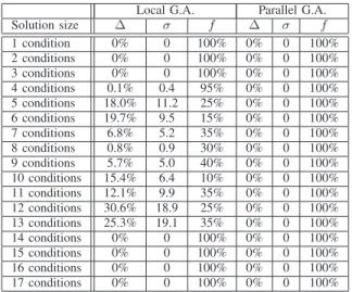
On small dataset such as the Kasumi Cell Line [29], the genetic algorithm performs very well, and even a single run of the local implementation with a population of size equal to the number of conditions, (here, 𝑚 = 10), finds the best solution. However, as soon as the number of conditions in the dataset increasese (e.g. Yeast Cell Cycle [30], with 𝑚 = 17), the same local implementation is more limited and some solutions it provides are quite far from the optimum. The parallel implementation, (with local parameters unchanged and sixteen islands), still provides optimal solutions. To further demonstrate the interest of this parallel implementation, severals runs of each implementation are performed. Results are shown in Table 1. The local implementation finds each optimal solution in at least 10% of all runs, but just under half of them are identified every time. The parallel implementation, with a similar computation time, finds the best solutions every time. To improve the overall performance of the algorithm, a fifth evolution operator is added. An existing solution is randomly selected, and a local search performed: we add a condition and remove an active one, (to maintain the bicluster size), as long as the solution can be improved. For small microarray dataset, this operator does not improve the overall performance, as the parallel algorithm was already identifying the optimal solution for each bicluster size.
For large datasets such as the Lymphoma dataset (𝑚 = 96 [31]), the overall performance is significantly improved, and the algorithm outperforms the previous implementation over the whole search domain. It also compares very well with a
Local G.A. Parallel G.A. Solution size Δ 𝜎 𝑓 Δ 𝜎 𝑓 1 condition 0% 0 100% 0% 0 100% 2 conditions 0% 0 100% 0% 0 100% 3 conditions 0% 0 100% 0% 0 100% 4 conditions 0.1% 0.4 95% 0% 0 100% 5 conditions 18.0% 11.2 25% 0% 0 100% 6 conditions 19.7% 9.5 15% 0% 0 100% 7 conditions 6.8% 5.2 35% 0% 0 100% 8 conditions 0.8% 0.9 30% 0% 0 100% 9 conditions 5.7% 5.0 40% 0% 0 100% 10 conditions 15.4% 6.4 10% 0% 0 100% 11 conditions 12.1% 9.9 35% 0% 0 100% 12 conditions 30.6% 18.9 25% 0% 0 100% 13 conditions 25.3% 19.1 35% 0% 0 100% 14 conditions 0% 0 100% 0% 0 100% 15 conditions 0% 0 100% 0% 0 100% 16 conditions 0% 0 100% 0% 0 100% 17 conditions 0% 0 100% 0% 0 100%
Table 1. Average gapΔ to optimal solution, standard deviation𝜎 and frequency 𝑓 at which optimal solutions
are found.
heuristic method developed specifically for this dataset. The genetic algorithm obtains better solutions for small cluster sizes, (0-12 conditions), and similar solutions elsewhere, as shown in Figure 7. Another interesting result is that the profile obtained is largely conserved over multiple runs: 71 biclusters, (out of 96), are obtained at each run and 18 of the remaining 25 have a standard deviation smaller than 10% of the average solution obtained. The latter ones correspond to non-optimal low-energy solutions in which the algorithm gets “trapped”. Overall, these results suggest that most of the solutions identified are optimal for their respective bicluster size.
Figure 7. A single run of the “hybrid” algorithm significantly outperforms the “standard” parallel genetic algorithm overall, and the heuristic method in a specific region , (low bicluster sizes), and obtains results similar to that of this method elsewhere.
4. Conclusion
In this paper, we showed benefits of a complete cycle of in silico data analysis in drug development stages, starting from a workflow towards comparison and parameter investigation stage. We have demonstrated both feasibility and the advantages of combining this process with in
vitro development. The amount of possible analysis that
can be done by the modelling framework in terms of investigation of parameter influence on drug release is practically unlimited, allowing analysing model data from a variety of different perspectives.
Furthermore, HPC extension to the framework makes it more applicable for a wider set of problems, allowing a fast and cost-effective modelling solution. Depending on the size of the device simulated (mili-, micro- or nano-), appropriate parallelisation strategy can be chosen to maximise the utilisation of processing power available.
Similarly, we showed that high-performance computing can be used to significantly improve the efficiency of optimisation techniques such as genetic algorithms. Using the parallel structure presented in this paper, it is possible to combine ease of deployment, computing efficiency and problem solving accuracy.
This approach is suited to biological data, as highlighted in the paper, but is easily adapted to other complex datasets. Other evolutionary algorithms have for instance been applied to churn detection [32].
Increased availability and affordability of high-performance computing will facilitate the ongoing development of these methods, and will contribute to solving existing challenges in data analytics.
Acknowledgments
Financial support from the Irish Research Council for Science, Engineering and Technology (IRCSET), co-funded by Marie Curie Actions under FP7 (Dimitri Perrin), and through an “Enterprise Partnership Scheme” postgraduate scholarship with Sigmoid Pharma Ltd. as an Enterprise Partner (Marija Bezbradica), is warmly acknowledged.
The parallel simulations discussed in this paper were performed on computational resources provided by the Centre for Scientific Computing & Complex Systems Modelling (Sci-Sym, DCU) and by the Irish Centre for High-End Computing (ICHEC).
References
[1] N. Nakasato, “Oct-tree method on gpu,” 2009. [Online]. Available: http://arxiv.org/abs/0909.0541v1
[2] A. Stevenson, Y. L. Du, and M. E. Afrit, “High-performance computing on gamer PCs,” Ars Technica, 2011. [Online]. Available: http://arstechnica.com/science/2011/03/ high-performance-computing-on-gamer-pcs-part-1-hardware/
[3] D. Bader, “Accelerating drug discovery,” Scientific Computing World, vol. 123, no. 2012, pp. 30–31, 2012.
[4] K. Zygourakis, “Development and temporal evolution of erosion fronts in bioerodible controlled release devices,” Chemical Engineering Science, vol. 45, no. 8, pp. 2359–2366, 1990.
[5] A. G¨opferich and R. Langer, “Modeling of polymer erosion,” Macromolecules, vol. 26, no. 1993, pp. 4105–4112, 1993. [6] J. Siepmann, N. Faisant, and J.-P. Benoit, “A new
mathematical model quantifying drug release from bioerodible microparticles using monte carlo simulations,” Pharmaceutical Research, vol. 19, no. 12, pp. 1885–1893, 2002.
[7] A. Barat, H. J. Ruskin, and M. Crane, “3D multi-agent models for protein release from PLGA spherical particles with complex inner morphologies,” Theory in Biosciences, vol. 127, no. 2008, pp. 95–105, 2008.
[8] T. J. Laaksonen, H. M. Laaksonen, J. T. Hirvonen, and L. Murtom¨aki, “Cellular automata model for drug release from binary matrix and reservoir polymeric devices,” Biomaterials, vol. 30, no. 10, pp. 1978–1987, 2009. [9] M. Bezbradica, M. Crane, and H. J. Ruskin, “Parallelisation
strategies for large scale cellular automata frameworks in pharmaceutical modellings,” in Proceedings of 2012 International Conference on High Performance Computing and Simulation (HPCS2012), Madrid, Spain, July 2012. [10] U.S. Food and Drug Administration. [Online]. Available:
http://www.fda.gov/
[11] United States Pharmacopeia. [Online]. Available: http: //www.usp.org/
[12] M. Bezbradica, H. J. Ruskin, and M. Crane, “Modelling drug coatings: A parallel cellular automata model of ethylcellulose-coated microspheres,” in Proceedings of the International Conference on Bioscience, Biochemistry and Bioinformatics (ICBBB 2011), vol. 5, Singapore, February 2011, pp. 419–424.
[13] I. Martin and F. Tiradoi, “Relationships between efficiency and execution time of full multigrid methods on parallel computers,” IEEE Transactions on Parallel and Distributed Systems, vol. 8, no. 6, pp. 562–573, 1997.
[14] J. H. Holland, Adaptation in natural and artificial systems. MIT Press, 1975.
[15] J. Grefenstette, “Parallel adaptive algorithms for function optimization,” Technical report CS-81-19, vol. Vanderbilt University (TN), 1981.
[16] E. Cantu-Paz, “A summary of research on parallel genetic algorithms,” IlliGAL report 95007, vol. University of Illinois (IL), 1995.
[17] D. Levine, “A parallel genetic algorithm for the set partitioning problem,” Technical report ANL-94/23, vol. University of Illinois (IL), 1994.
[18] C. M. N. A. Pereira and C. M. F. Lapa, “Coarse-grained parallel genetic algorithmnext term applied to a nuclear reactor core design optimization problem,” Annals of Nuclear Energy, vol. 30, no. 5, pp. 555–565, 2003.
[19] K. Katayama, H. Hirabayashi, and H. Narihisa, “Analysis of crossovers and selections in a coarse-grained parallel genetic algorithm,” Mathematical and Computer Modelling, vol. 38, no. 11-13, pp. 1275–1282, 2003.
[20] F. Valafar, “Pattern recognition techniques in microarray data analysis: A survey,” Annals of the New-York Academy of Sciences, vol. 980, no. 1, pp. 41–64, 2002.
[21] G. Stolovitzky, “Gene selection in microarray data: the elephant, the blind men and our algorithms,” Current Opinion in Structural Biology, vol. 13, pp. 370–376, 2003.
[22] S. Raychaudhuri, P. D. Sutphin, J. T. Chang, and R. B. Altman, “Basic microarray analysis: grouping and feature reduction,” Trends in Biotechnology, vol. 19, pp. 189–193, 2001.
[23] D. K. Slonim, “From patterns to pathways: gene expression data analysis comes of age,” Nature Genetics, vol. 32, pp. 502–508, 2002.
[24] Y. Cheng and G. M. Church, “Biclustering of expression data,” in Proceedings of the 8th International Conference on Intelligent Systems for Molecular Biology (ISMB 2000), vol. 8, San Diego, California, USA, August 2000.
[25] R. Peeters, “The maximum edge biclique problem is NP-complete,” Discrete Applied Mathematics, vol. 131, no. 3, pp. 651–654, 2003.
[26] G. Kerr, D. Perrin, H. J. Ruskin, and M. Crane, “Edge weighting of gene expression graphs,” Advances In Complex Systems, vol. 13, no. 2, pp. 217–238, 2008.
[27] D. Perrin, C. Duhamel, H. J. Ruskin, and M. Crane, “Microarray biclustering: mathematical model and metaheuristic alternatives,” in International Conference on Computational Methods (ICCM 2007), Hiroshima, Japan, April 2007.
[28] C. Duhamel and D. Perrin, “Genetic algorithms to compute a set of bicliques in microarray biclustering,” LIMOS, Tech. Rep. RR-08-07, 2008.
[29] Gefitinib Treated Kasumi Cell Line Dataset, MIT Broad Institute. [Online]. Available: http://www.broad.mit.edu/ cgi-bin/cancer/datasets.cgi
[30] Yeast Cell Cycle, available from R.W. Davis’ website at Stanford. [Online]. Available: http://genomics.stanford.edu/ yeast cell cycle/cellcycle.html
[31] Lymphoma/Leukemia Molecular Profiling Project Gateway. [Online]. Available: http://llmpp.nih.gov/lymphoma/ [32] W.-H. Au, K. C. C. Chan, and X. Yao, “A novel evolutionary
data mining algorithm with applications to churn prediction,” IEEE Transactions on Evolutionary Computation, vol. 7, no. 6, pp. 532–545, 2003.