Annular modes in multiple migrating zonal jet regime

Annular

Modes in

a Multiple Migrating

Zonal

Jet Regime

Cegeon

J

Chan

B

.S., Meteorology;

B

.S.

Mathematics Lyndon State College, 2003

Submitted to the Department of Earth, Atmospheric, and Planetary Science in Partial Fulfillment of the Requirements for the Degree of

Master

of

Science

in

Atmospheric Science

OF TECHNOLOW

at the

Massachusetts Institute of Technology

_I

_-

₁

I

February 2006

\

LIBRARIES

I

@ 2006 Massachusetts Institute of Technology

All rights reserved.

ARCHMES

I

Signature of Author..

...

.-. .

.r..

...

:

...

'

_{Department of Earth, Atmospheric, and Planetary Science}

January 25,2006

-

...

Certified by..

...

R. Alan Plumb Professor of Earth, Atmospheric and Planetary Science Thesis Supervisor

Accepted by

...

,K

....

IKP

....

:

...

f . .

...

Maria T. Zuber

E.

A. Griswold Professor of Geophysics Head, Department of Earth, Atmospheric and Planetary Sciences

Annular Modes in a Multiple Migrating Zonal Jet Regime

Cegeon J Chan

Submitted to the Department of Earth, Atmospheric, and Planetary Science on January, 25, 2006, in partial fulfillment of the

requirements for the degree of Master of Science in Atmospheric Science

Abstract

Recent studies have linked hemispheric climate variability to annular modes, zonally symmet- ric structures that describe the horizont a1 redistribution of atmospheric mass. The resulting changes in the pressure patterns consequently alter the atmospheric circulation, including the movement of zonal jets in the atmosphere. While the literature contains much observational evidence describing these annular modes, the fundamental dynamics in the perpetuation of the annular modes still remains poorly understood.

We investigate the dynamics of the annular modes using the MITGCM, a semi-hemispheric ocean model. The forcings imposed in the model are an atmospheric wind stress and re- laxation to a latitudinal temperature profile, which induces a baroclinically unstable flow. Despite such an idealized setup, the model output shows striking similarities to the observed atmospheric annular modes, where the leading mode of variability is associated with the primary zonal jet's meridional displacement. By convention, when the zonal jet is poleward (equatorward) of its time-mean position, the principal component (PC) of the first empirical orthogonal function (EOF) is positive (negative) and is referred to as the high (low) zonal index.

In the model, systematic secondary (weaker) jets migrate equatorward into the primary jet. The total eddy forcing associated with the migrating jets aids in sustaining the primary jet in the presence of frictional forces. Plots of the anomalous eddy fields for both indexes show that the strongest eddy activity in the main jet is associated with the high zonal index. The zonal flow anomalies, which systematically migrate into the poleward flank of the main jet, are largely responsible for causing this positively anomalous eddy forcing. This asymmetrical forcing to the primary jet results in the zonal index variability.

In this thesis, the dynamics associated with the secondary jets and its equatorward migration will be examined. We will show that when (1) the sphericity of the earth is accounted for, (2) the interior PV is homogenized, and (3) the width of the baroclinically unstable region exceeds the Rhines scale by several factors, multiple zonal jets emerge and migrate equatorward.

Thesis Supervisor:

R.

Alan Plumb Title: Professor of Meteorology

Acknowledgments

Particularly at an university like MIT, graduate programs are setup to test and challenge the students' ability to perform independently. However, one cannot earn a degree without the support from others. The following are the people who have helped me along the way.

First, I would like to thank my advisor, Alan Plumb for frequent insightful discussions. He has helped guide me through my wrong turns and helped me stay on the right course. Despite his busy schedule, I appreciate his ability to always find time for me.

My fellow classmates have always been friendly and have supported the last couple of years. In particular, I would like to thank Yang Zhang, Daniel Enderton, Ian Fenty and Bhaskar Gunturu for our Friday afternoon sessions in the Spring of 2005 working together to prepare for the dreaded General Exam. Their help made the process less daunting. Also, my officemates - Dave Flagg, Vikram Khade, and Kelly Klima - were pleasant to talk with

when a break from work was in order.

This thesis would not be possible without the people in my research group - Will Heres,

Nikki Privk, Mike Ring, and Ivana Cerovecki. Nikki was my "mentor" and was an excellent resource for advice as a first-year graduate student. Mike provided useful comments that benefitted this thesis, and Ivana always had an answer for any question I had pertaining to the model output and to the MITGCM itself.

Outside of this department, a special thanks go to Jason Furtado and Vivian Cheng. As a friend and colleague from our undergraduate days and now graduate school, Jason has not only helped contribute insightful comments to this thesis, but I have also benefitted from

many fruitful discussions about a variety of topics in our field. Finally, Vivian Cheng, my girlfriend of seven years, has had to put up with the roller coaster ride associated with being a graduate student and its time constraints. She has always been right beside me and been able to provide balance to my often idealistic views of the world with much needed practical perspectives.

This material is based upon work supported by the National Science Foundation under Grant No. 03 14094. Any opinions, findings, and conclusions or recommendations expressed in this material are those of the author and do not necessarily reflect the views of the National Science Foundation. Lastly, I also acknowledge the financial support from the NASA's Earth Science Enterprise Graduate Fellowship.

Contents

1 Introduction . . . 1.1 Annular modes 13 . . . 1.2 Zonal Jets 15 . . . 1.3 Motivation 18 2 Setup 21 . . . 2.1 Model 21 . . . 2.2 Methodology 25

3 Climatology of the MITGCM

4 Description of Variability 36

. . .

4.1 EOF Analysis 38

. . .

4.2 Description of EOF phases 41

5 Eddy Properties 47

. . .

5.2 Eddy Effects.

.

.

. . . . .

. . .

. . . .

.

. . . . .

. .

. .

.

. . . . . . . . . .

51

. .

5.3 Momentum Budget

. . . . .

.

.

.

. . .

.

. . . .

.

. . . . . . . .

57

6 Comparison t o Simple Models 62

6.1 Frictional Effects

. .

.

. . . . .

.

. . .

.

. . .

. . .

. . . . .

.

.

.

.

. . . .

.

62 6.2 Sphericity Effects

.

. . . . . . . . .

.

. . . . . .

.

;

. .

. .

. . .

.

.

. . .

66 6.3 Sphericity and Frictional Effects . .

. .

.

. . . . .

.

.

. . . .

.

. . . . . . . .

67

7 Discussion 71

7.1 Migrating Jets

. .

.

. . . . .

. .

. . . .

. .

. . . . . . . . .

. . .

. . . .

71 7.2 Zonal index variability .

. . . .

. . . .

.

. .

. . .

. . . . . .

.

. .

. . . . . .

76

8 Conclusion 79

8.1 Future Work. .

. . . .

. .

. . . . . .

.

. . . . . .

. . .

. . . . . . . . .

.

. .

81

List

of

Figures

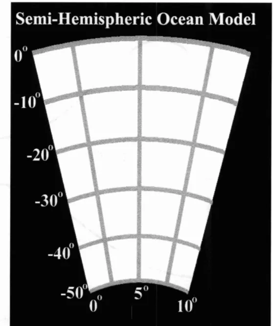
2.1 Model's domain ranges from 50.67"s to 0.17"s and OOE to 10" E and periodic in the zonal direction on a

i0

x

i0

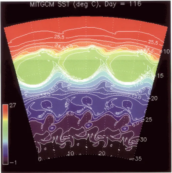
latitude/longitude grid. See text for details. 23 2.2 Model-prescribed forcings. (a) Atmospheric wind stress. (b) Specified temper-

ature profile with a relaxation time of order one month. Note: both forcings are const ant in time, only a function of latitude, and applied to the top surface layer (22m). . . 24 2.3 Snapshot of the horizontal temperature distribution. For visual purposes,

since the model is periodic in the zonal direction, the graphical output between 10" and 30" are duplicates of that for 0 - 10". . . 26 2.4 Time series of [u(y,

z ,

t ) ]

.

Time stamps (in years) are located on bottom left

corner of each plot.

. . .

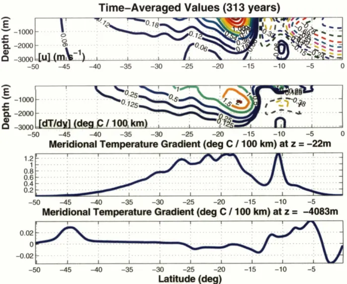
28

3.1 Model's time and zonally-averaged values for (a) zonal flow, (b) meridional temperature gradient, (c) meridional temperature gradient at the top bound- ary and (d) lower boundary. . . . 30

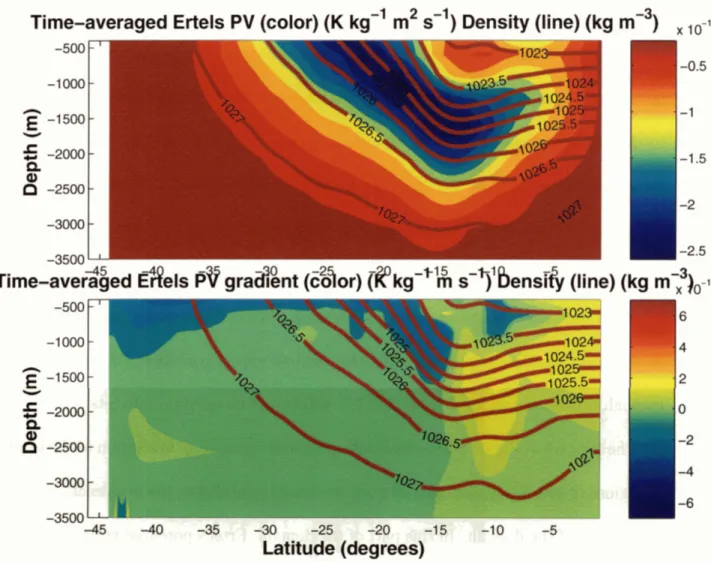
Model's time and zonally-averaged values for Ertel's potential vorticity (top) and its meridional gradient (bottom) along isopycnals.

. . .

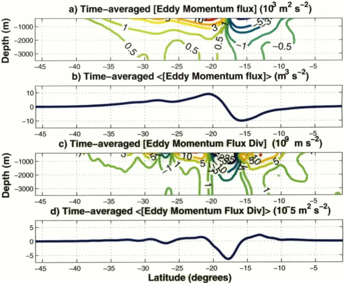
Time and zonally-averaged values for (a) the eddy momentum flux (b) vertically- integrated eddy momentum flux (c) eddy momentum flux divergence (d) vertically-integrated eddy momentum flux divergence.

. . .

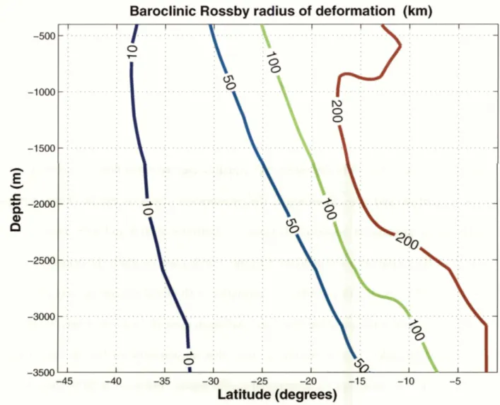
Baroclinic Rossby radius of deformation.

. . .

Time series of the anomalous vertically-integrated zonally-averaged zonal flow. Positive contours start at 20 and increase in increments of 200. Negative contours (dashed lines) start at -200 and are also in increments of 200.

. . .

The first three leading EOFs of the annually-averaged zonal-mean zonal flow. Solid (dashed) lines represent positive (negative) values. Black vertical line indicates position of the time-averaged jet. Percent variance accounted is shown a t bottom right corner.

. . .

Principal components of the first and second EOF modes. . . Time series of the reconstructed zonal flow using the leading two modes

-

(u,,, - u,,,,

+

PC1 • EOFl

+

P C 2

.

EOF2).

. . .

(a) Graphical display of the EOF phases. Note the abscissa is PC1 and the ordinate is PC2. (b), (c) and (d)

A

time series of the jet characteristics as described by the EOF phases.

. . .

Eliassen-Palm cross sections. The total E P flux vectors for each EOF phase (labelled on bottom left corner) are plotted over zonally-averaged zonal flow.

5.2 Anomalous Eliassen-Palm cross sections. Anomalous E P flux vectors for each EOF phase are plotted over the zonally-averaged zonal flow anomalies. Each phase is labelled at the bottom left corner of plot.

. . .

55 5.3 Same as Fig. 5.2 but with the flow tendency contoured instead. . . . 56 5.4 (a) Time-averaged quantities of the vertically-integrated zonal momentum

budget. (b) Time-average of the vertically-integrated eddy momentum flux

<

[u'v']

>.

. . . 59 5.5 Terms to the vertically-integrated zonal momentum balance for (a) year 1296

and (b) year 1298. Vertically dashed lines correspond to maximum zonal flow anomalies.

. . .

60

6.1 Simple model of flow tendency balancing both the eddy and frictional forces for (a) the inviscid case with CD = 0, (b) "slight friction case" with CD = 0.3, (c) "moderate friction case" with CD = 3.0 and (d) "extreme friction case" with CD = 9.0. . . . 65 6.2 Simple model with (a) symmetric wave activity, (b) symmetric eddy forcing,

(c) asymmetric wave activity with an equatorward bias and (d) asymmetric eddy forcing with an equatorward bias. . . . 68

6.3 Simple model combining the effects of friction and sphericity. The meridional value of zero has been arbitrarily been defined as the equator. For all time steps, the maximum forcing is prescribed to have the same spatial relationship as the zonal flow, but shifted slightly equatorward. The top three plots show the flow tendency, the zonal flow, the eddy forcing and friction at the particular time frame. The bottom plot indicates the zonal flow as a function of space and time.

. . .

69

7.1 A snapshot of a) zonal anomalies and b) of the anomalous horizontal EP flux at t = 1008 years. A snapshot of c) zonal anomalies and d) of the anomalous horizontal EP flux at t = 1012 years.

. . .

73 7.2 Anomalous horizontal EP flux (line) for each

EOF

phase plotted over zonally-

averaged zonal flow anomalies (in color).

. . .

74 7.3 Total eddy forcing for the high and low zonal index. As reference, the time-

Chapter

1

Introduction

1.1

Annular modes

Modes of climate variability in the atmosphere have long been studied. Calling it the North Atlantic Oscillation (NAO), Walker and Bliss (1932) demonstrated negative correlations in pressure between the North Atlantic and the subtropics of Europe. Meanwhile, Rossby (1939) introduced the zonal index as a measure of the strength of the mid-latitude westerlies between 35" N and 55" N. Namias (1950) went further by proposing the fluctuations in the flow strength was associated with the "zonal index cycle,'' an oscillation owing to the jet's meridional displacement. Lorenz (1951) then linked the two latter ideas together by averaging the zonal-mean zonal flow at 55"N and using it as a proxy to measure the pressure oscillation.

In more recent years, Thompson and Wallace (1998), who first used the term "annular modes", described the leading mode of variability as a seesaw of mass between mid- and

high-latitudes similar to Walker and Bliss (1932). However, Thompson and Wallace (1998) expanded the regional analysis to include the entire hemisphere. They showed that there was a stronger connection between the variability of the wintertime Eurasian surface air temperatures with the leading mode of the hemispheric zonal-mean sea-level pressure rather than to the regional fluctuations associated with the NAO. M h e r m o r e , other studies (e.g. Limpasuvan and Hartmann 2000) have demonstrated that this leading mode of variability is not only annular-like, but is barotropically equivalent, i.e. the pattern extends from the surface up to the tropopause and amplifies with height.

Although annular modes are observed in both hemispheres, Lorenz and Hartmann (2001), hereafter LHO1, analyzed the Southern Hemisphere (SH) annular mode (SAM) which is more zonally symmetric and provides more robust results than its northern counterpart. They showed that anomalously high pressure in the mid-latitudes is associated with a poleward shift of the jet and, conversely, anomalously low pressure in the mid-latitudes is associated with an equatorward shift of the jet. By convention, a poleward shift of the jet corresponds to a high index phase while an equatorward shift is defined as a low index phase.

Lorenz and Hartmann (2001) described the jet displacement as the leading mode of zonal- mean zonal flow variability through the first empirical orthogonal function (EOF) of [u]. Its dipole structure, with local maximum and minimum anomalies centered about ten degrees north and south of the time-averaged maximum wind speeds, captures the "wobbling" or meridional displacement of the zonal jet. The second EOF coincided with the location of the mid-latitude jet representing the strengthening and weakening of the jet, or similarly the

jet narrowing and broadening of the jet.

The time-scales associated with these modes can range from intra-seasonal to decadal (Thompson and Wallace 1998). Therefore, annular modes can be helpful to describe climate change. For example, Hurrell (1995) showed a strong correlation with surface air temperature with the annular modes over the previous 30 years. Thompson and Wallace (2000) also show that the Northern Annular Mode (NAM) index trended toward a persistent positive phase in the late 1980s and throughout the 1990s, consistent with trends in the NAO (e.g. Hurrell 1995).

1.2

Zonal

Jets

The reasoning behind examining ring-like structures for low-frequency behavior can be at- tributed to many processes. But primarily, based on the theories of geostrophic turbulence in barotropic fluids and conservation of energy and enstrophy, kinetic energy is transferred from high wave numbers to low wave numbers, while enstrophy cascades from low wave numbers to high wave numbers, where it dissipates (Pedlosky 1987). The effect of the inverse energy cascade creates spatially larger eddies. In the absence of other forces such as rotational and frictional forces, eddies will grow to the size of the domain.

Rhines (1975) described how the P-effect can halt the cascade of energy to larger scales. As the eddies grow in size, variations of planetary vorticity increase in importance, and when eddies are sufficiently large, the effect of Rossby wave dynamics will be approximately equal to nonlinear interactions. Ram the barotropic vorticity equation shown below, a scaling

argument shows the length scale at which a turbulent regime turns more dynamically wave- like.

where ( is the relative vorticity, u' is the velocity, and v the meridional speed.

The second term scales as and the third term scales as

PU.

For small scales, the advective term dominates, and for large scales, the ,8-term dominates. When the two terms are in "balance", it is called the Rhines scale:

In the meridional direction, the Rossby wave frequency is inherently anisotropic, therefore flows organize themselves into zonal structures (Rhines 1975). This can be attributed t o the general tendency for the energy to seek the gravest mode and hence cascade toward low zonal wavenumbers (Vallis and Maltrud 1993). In essence, this process "flattens" the eddies in the north-south direction and turns them from isotropic to anisotropic. Therefore, the final process of the cascade leads to longitudinally oriented eddies producing zonally symmetric jet-like flows (Rhines 1975).

Adjusting to a baroclinically unstable regime, Held and Larichev (1996) used a scaling

argument to come up with an adjusted "baroclinic" version of the Rhines scale, &) =

9,

where ii is the baroclinic eddy velocity and LD is the baroclinic Rossby radius of deformation. Therefore, if the domain size is larger than this scale, the possibility for more than one

zonal jet can exist. Furthermore, numerical studies (e.g. Williams 1978) have shown if the baroclinically unstable region greatly exceeded the Rhines scale, multiple jets develop.

Panetta (1993) imposed an unstable horizontally uniform vertical shear over several tens of Rossby radii wide with a quasi-geostrophic (QG) two-layer P-plane model to test for the existence of multiple jets. Given dissipation was sufficiently weak, multiple jets emerged and were demonstrated to be remarkably persistent. By using a full zonal and meridional spectrum, Panetta (1993) also showed the existence of multiple jets was not a consequence of leaving out long zonal waves i.e. low model resolution did not lead to fabrication of zonal jets.

Panetta recognized the earth's ocean, where the Rossby radius of deformation is an order of magnitude smaller than the atmosphere, would allow for multiple jets to be observed e.g. the Antarctic Circumpolar Current (ACC). Using a QG channel model forced by a surface wind stress, Treguier and Panetta (1994) found multiple jets would emerge given a limited amount of curvature to the meridional wind stress.

These numerical studies by Williams (1978), Panetta (1993) and Treguier and Panetta (1994) were all done using a quasi-geostrophic (QG) model. Expanding upon the hierarchy of models simulating multiple jets, Lee (2005) utilized a primitive equation model on a spherical planet. Varying the size of the planetary radius and baroclinic intensity, Lee demonstrated the meridional scale of the jet was consistent in each case with the Rhines scale.

1.3

Motivation

The above studies of multiple jets have been based on simplified models such as QG models on a ,@-plane. Only through modelling multiple jets with different levels of model complexity can theories be rigorously tested. Our use of the MITGCM serves multiple purposes. Since the MITGCM uses spherical coordinates, the model captures the earth's latitudinal variations of the earth's curvature. It can be shown that the group velocity is proportional to eddy momentum fluxes (Andrews et al. 1987). Therefore, Rossby waves have a bias in propagating equatorward (e.g. Whitaker and Snyder 1993; Limpasuvan and Hartmann 2000). Under this framework, this will lead to asymmetric forcing in relation to the zonal jet that models using a ,@-plane omit.

This work was primarily motivated by the output from a ocean model run from the MIT- GCM. Similar to previous studies, the setup is such that width of the baroclinic region is much larger than the baroclinic Rossby radius of deformation. However, secondary (weaker) jets are observed to systematically migrate equatorward. The author is not aware of such behavior being reported previously. Since the model-imposed forcings are constant in time with flat-bottom topography, it is the internal dynamics most likely responsible for estab- lishing the remarkable persistence of the migrating zonal jets. This equatorward bias in the zonal anomalies is in contrast to the poleward propagation of the zonal anomalies observed in the atmosphere (Feldstein 1998).

Along with addressing this issue, another goal of this work is to describe and explain the annular mode-like behavior associated with this model run. The leading mode of variability of

the zonally-averaged zonal flow describes the meridional displacement of the primary jet, very similar to the observed atmosphere (e.g. Lorenz and Hartmann 2001). The model-imposed forcings here are constant in time, but yet, there is still temporal variability associated with the zonal jets. The most likely explanation can be attributed to the eddy effects on the zonal-mean flow.

Yu and Hartmann (1993) conducted a modelling study with a GCM and determined the convergence of the transient eddy momentum flux is important in not only maintaining a meridionally displaced jet, but also in the transition from one zonal index to another. This implies a momentum budget analysis is important to show that the eddy momentum flux convergence is the major forcing in both the extreme and transitional phases. It would be of interest to compare eddy statistics given our regime of migrating jets.

We note that the two forcings to the model have been idealized. The model-imposed wind stress does not account for easterlies in the tropical atmosphere, i.e. there are only westerlies in mid-latitudes and the wind stress tapers off equatorward. The requirements needed for such conditions (if even plausible) will not be discussed here. However, a cursory description of the model will be presented in section 2, and in section 3, we will perform a time-average of certain diagnostics in order to examine the climatology of the model. Then, we will analyze the spatial and temporal variability by utilizing empirical orthogonal functions (EOFs) in section 4. Descriptions of the eddy properties will be presented and discussed in section 5. In section 6, a comparison will be made between some our GCM results and simple models. A discussion on our results will be given in section 7. Finally, we conclude with a summary

Chapter

2

Setup

2.1

Model

The data in this study were generated from the MIT General Circulation Model (MITGCM).

A

more complete description of the MITGCM can be found in Marshall et al. (1997a, 1997b). Here we provide just a cursory description of the model setup.

This is a semi-hemispheric model ranging from 50.67"s to 0.17's and OOE to lo0 E periodic in the zonal direction on a

i0

x

i0

latitude/longitude grid. There are 15 vertical layers with each layer's depth ranging from approximately 22m in the first top six layers to approximately 400m for the bottom nine layers.

A

two-dimensional sketch is shown in Figure 2.1.

The simulated ocean varies from the actual ocean in a number of ways. Boundaries such as continents and topography that could potentially influence the flow have been ignored. The model does not account for trade winds, i.e. only westerlies with the wind tapering off

towards the equator are considered.

In the absence of such boundaries, the model has been setup to be a zonally reentrant channel. The periodic boundary conditions in the zonal direction are, in general, more rep- resentative of the atmosphere than the ocean and may facilitate annular mode-like structure similarly observed in the atmosphere. However, unlike the atmosphere, the fluid is chan- nelled between two walls. Free-slip and no-slip boundary conditions are used at the equator and at 50.5OS, respectively.

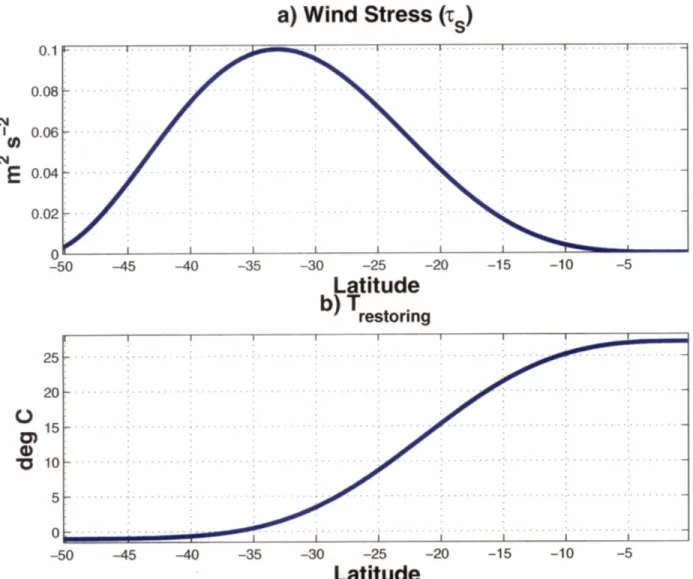
The model-imposed forcings include a wind stress (Figure 2.2a) and a heat forcing (Figure 2.2b). Both forcings are constant in time, a function of latitude only, and applied only to the top layer of the ocean. Compared with the oceanic Rossby radius of deformation (which is in the order of 50 km), the width of the forcings are extremely broad.

For our oceanic case, this wind stress acts as our source of momentum from the at- mosphere into the ocean's top layer, with the peak located at 33's. When the model starts integrating, the wind stress will cause the top layer's zonal flow to increase with time. After a sufficient length of time, the flow becomes baroclinically unstable, perturbations grow, and eventually, eddies transfer moment um equat orward and downward, until eventually momen- tum is then removed out of the system at the ocean's bottom due to bottom drag.

The second applied forcing is a model-imposed temperature profile. The restoring time for this heat forcing, shown in Figure 2.2b, to return to the specified temperature profile is of order 1 month. Thus this heat forcing is associated with warming close to the equator and cooling to the south. This semi-realistic forcing is also constant in time and independent of

Figure 2.1: Model's domain ranges from 50.67"s to 0.17OS and OOE to 10" E and periodic in the zonal direction on a $" x $" latitude/longitude grid. See text for details.

a)

Wind

Stress

(7,)

Latitude

b,

Trestoring 0 -50 -45 -40 -35 -30 -25 -20 -1 5 -1 0 -5

Latitude

Figure 2.2: Model-prescribed forcings. (a) Atmospheric wind stress. (b) Specified tempera-

ture profile with a relaxation time of order one month. Note: both forcings are constant in

longitude.

The size of any eddies is always limited to size of the particular model's domain. Part of the model's domain size is shown in Figure 2.3. In certain parts, the 10" width of the channel likely stopped the inverse energy cascade. Between 12"s and 17"S, an eddy fills the entire latitude circle and has most of its energy in wave number 1. It is likely if given a sufficiently larger zonal domain, the eddy would have been horizontally larger and appear less isotropic i.e. more zonal as described by Rhines (1975).

The depth of the ocean is 4083m, and the model's bottom drag is specified to be:

where

A,

is the vertical viscosity, U M is the zonal velocity at the bottom of the ocean, rbot

is the thickness of the bottom layer, KE is the kinetic energy and

CD

is the bottom drag coefficient.

2.2

Methodology

With the lack of any longitudinally asymmetric forcing, it is appropriate to consider zonal mean budgets. Therefore, since we are interested in the low-frequency behavior, unless otherwise noted hereafter, quantities displayed in this paper have been annually and zonally- averaged and will be denoted with square brackets.

Figure 2.3: Snapshot of the horizontal temperature distribution.

For

visual purposes, since the model is periodic in the zonal direction, the graphical output between 10" and 30" are

we use the principal component (PC) of the leading empirical orthogonal function

(EOF)

of the zonally-averaged zonal flow to define the "zonal index." As we shall see, the first EOF describes the north-south displacement of the jet. Positive (negative) values of the PC indicate a poleward (equatorwasd) shift of the jet and will be referred to as a high (low) phase of the zonal index.

Figure 2.4 displays the time series of the annually and zonally-averaged flow over a nine- year period. The flow is strongest between 15"s and 20"s and closest to the surface with peak values approximately 2.5 ms-'. Poleward of 20°S, weaker zonal jets develop around 35"s and migrate equatorward. The zonal jet between 15"s and 20"s will be referred to as the primary jet, and zonal jets poleward of 20"s will be called secondary jets.

Zonally averag

-

d

zonal

flow

(m

s-I)

Figure 2.4: Time series of [u(y

,

z,

t ) ]

.

Time

stamps (in years) are located on bottom left

Chapter

3

Climatology of the MITGCM

The 313-year time series of the zonal-mean zonal flow [u(y, 2,

t ) ]

shown in Figure 2.4 can be

split into two parts: the time mean [fi(y, z ) ] and its deviations, [uf(y, 2,

t ) ] .

In this section,

we focus on the former. The top plot of Figure 3.1 shows the latitude-depth plot of the zonal-mean zonal flow. This time-averaged plot shows the highest zonal flow values located between 15"s and 20°S, with the primary jet centered at 17's. Poleward of this primary jet, time-averaged zonal flow speeds appear to be about an order of magnitude less. As shown in Figure 2.3, the period for secondary jets migrating into the primary jet is approximately 10 years. Therefore, because of the migrating jets, such a long time-average (313 years) smooths out the zonal flow south of 20"s. Nevertheless, there is still a hint of another zonal jet at 27's.

The mean meridional temperature gradient, shown in the second plot of Figure 3.1, has its largest values coinciding with the strong jet as expected by thermal wind balance. The meridional temperature gradient extends through the vertical, damping as we progress

Time-Averaged

Values

(31

3 years)

-50 -45 -40 -35 -30 -25 -20 -1 5 -10 -5 0

Meridional

Temperature

Gradient

(deg

C

/

100

km)

at

z =

-22m

-50 -45 -40 -35 -313 -25 -20 -1 5 -1 0 -5

Meridional

Temperature Gradient

(deg

C

1

100

km)

at z

=

-4083m

-50 -45 -40 -35 -30 -25 -20 -1 5 -10 -5

Latitude

(deg)

Figure 3.1: Model's, , w e and zonally-averaged values for (a) zonal flow, (b) me temperature gradiedt, ' ( c ) meridional temperature gradient at the top boundary

-1 2

Time-averaged

Ertels

PV

(pdor)

(K kg

m

s-I)

Density

(line)

(kg

m-3)

-( l o - l ~

- - - -

~ime-aver$&ed

Edels

PV

gradgnt

(=%or)

(f

kg-''&

s-9'

bensifY

(line)

(kg

m;3)0--16

EO

-45 -40 -35 -30 -25 -20 -15

Latitude

(degrees)

! I ,417 $; r.,uL* * ' sm

Figure 3.2: Model's t i m

lurd

a v e r a d values for Ertel's potential vorticity (top) and

its meridional gradient ;&bottomJ along isopycnals. , , ,

,

, , , , , ,

I b$

downward,

co

e ~ ~ ~ t i 3 h t i W a r o t r o ~ c structurb This implies that the

have the same sign along the top and battom boundaries

as

s h m n in Figures

3.

lc and 3. ld

between' SU;5° and 26"s and loliolates thslf marney-Sternt sufficient ~ondition for st ability.

However, this is

nat

% h m o s t obvious way to examine the system's stability.

In Figure

ta;

*&teTb potential vortieity 'is plotted dong lines of constant density.

1

one would expect this region to be stable. This is consistent with the applied wind and heat forcings (Figure 2.la and 2.lb) as they are both tapered off towards the equator. With no westward wind stress towards the equator, there is no upwelling (significant enough) to disturb the isopycnals in this equatorial region. In addition, since the heat forcing is rather smooth equatorward of 10°S, the westerly wind stress was tapered to prevent inertial instability and upwelling near the equator. This region, equatorward of 10°S, is stable.

Poleward of 14"S, the time-averaged isopycnals have significant slopes with comparison to height surfaces. Therefore, there is available potential energy for any perturbations to grow. This region is baroclinically unstable, and we expect baroclinic eddies to develop, and through processes explained in section 1.2, will funnel momentum into jets.

The top plot of Figure 3.2 shows Ertel's potential vorticity, q, in relation to the isopycnals. In regions of instability, contours of q are remarkably parallel to the isopycnals, especially in the interior of the domain. In this part of the domain, Ertel's potential vorticity has become homogenized along the time-averaged isopycnals. The likely mechanism in smoothing q can be attributed to eddies transporting PV downgradient (see Rhines and Young 1982; Kuo et al. 2005 ). The bottom plot emphasizes the point that Ertel's PV gradient (along isopycnals) is virtually zero in the interior.

The time-mean of the eddy momentum flux is shown in Figure 3.3a and Figure 3.3b. Poleward (equatorward) of the primary jet, momentum is being transferred equatorward (poleward.) Figure 3 . 3 ~ and Figure 3.3d shows that almost all of the time-mean horizon- tal momentum flux converges at the primary jet. There is a hint of another convergence

maximum region centered at 27's where another secondary jet is observed (see Fig 3. la). This is consistent with a study done by Held and Andsews (1980). The authors' have shown that flows with a horizontal jet structure broader than the Rossby radius of deforma- tion will have a vertically-integrated momentum flux into the jet. For our study, the Rossby radius of deformation (see Fig 3.4) is on the order of about 100 km, while the primary jet length scale is about 500 km and as shown, in Fig 3.3d, there is a convergence of eddy mo- mentum flux. This is likely to be the mechanis~n that sustains the jet even in the presence of frictional forces. This will be discussed further i11 section 5.3.

2 -2

a)

Time-averaged

[Eddy Momentum

flux]

(I$

m

s

)

n

E

-1000 w

5

-2000

a

8

-3000 -45 -40 -35 -30 -25 -20 -1 5 -1 0 -5 3 -2

b)

Time-averaged

<[Eddy

Momentum

flux]>

(m

s

)

-45 -40 -35 -30

-

t -20 -1 5 -10 -5

c)

Time-averaged

[ ~ d d y

I

amenturn

Flux

Div]

(18

m

sw2)

-45 -40 -35 -30 -25 -20 -1 5 -10 259

d)

Time-averaged

<[Eddy

Momentum

Flux

Div]>

(I(r5

m

s

)

-45 -40 -35 -30 -25 -20 -1 5 -1 0 -5

Latitude

(degrees)

Figure 3.3: Time and zonally-averaged values for (a) the eddy m o m t u r n flux (b) vertically- integrated eddy momentum flux (c) eddy momentum flux

divergence

(d) vertically-integrated eddy momentum flux divergence.

Baroclinic

Rossby

radius

of

deformation

(km)

-. Figure 3.4: Baroclinic Rossby radius of defoimat ion.

Chapter

4

Description of Variability

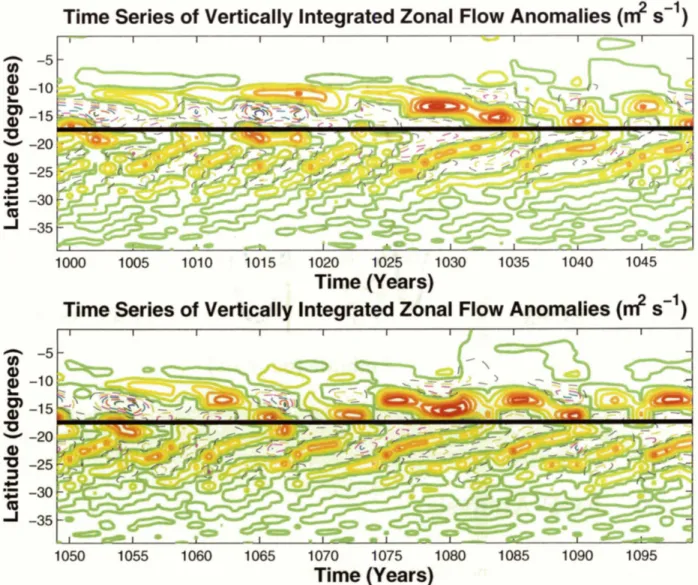
Figure 4.1 shows the vertically-integrated, zonally-averaged zonal flow anomalies as a func- tion of latitude and time. Once again, the equatorward migration can be clearly seen pole- ward of the primary jet, especially between the latitudes of 20"s and 30"s. From the emer- gence of the secondary jet around 30"s to the time it takes to reach the primary jet ranges from 8 to 12 years. In other words, the translation of the zonal jets are not constant, i.e. the migration speed of the zonal jets fluctuate. Although most of our focus is between the above mentioned latitudes, it is interesting to note that an equatorward bias in the anomalous zonal-mean flow anomalies isn't restricted to this region. Poleward of 30°S, there are weak zonal anomalies that also show an equatorward bias and exhibit similar migration speeds as the stronger secondary jets.

Time

Series

of

Vertically

Integrated

Zonal

Flow

Anomalies

(d

so')

1070 1075 1080 1085

Time

(Years)

ll';

14. I I ,

Figure 4.1: Time series of the iuiomalous vertically-integrated zonally-averaged zonal flow.

Positive contours start at 20 and increase in increments of 200. Negative contours (dashed lines) start at -200 and are also in increments of 200. ' ; j r ,

-20 -1 5

Latitude

(degrees)

Figure 4.2: . m e '

6&t

threei%ang

'EOFs

of

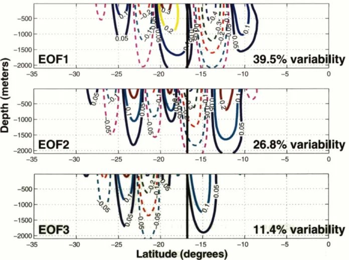
the annu&-averaged z&kl-mean zon& flow.

Solid (dashed) lines represent positive (negative) values. Black vertical line indicates position

of the time- .jet.

Pw&

uuiarxe

accowed is

$bCm

at

b&tm

pgbt corner.

EOjF

Analysis

The spatial and temporal variability of the zonally-averaged zonal flow can be best summa-

rized by the use of empirical orthogonal functions (EOFs) as shown in Figure 4.2. The data

was weighted to account for the decrease in area around latitude circles toward the pole, but

was not weighted to account for the varying vertical layer depths. However, this shall not

be important as we are interested in the horizontal variations of the zonal flow. Using the

EOFl shows an equivalent barotropic structure with maximum anomalies at 19's and 14's. The black line represents the time-averaged location of the jet's maximum value (17.2'5). By comparing the variability of this mode and the mean location of the jet, we determine that EOFl physically represents the meridional fluctuations of the main jet, or in other words, EOFl captures the jet "wobbling" in the north-south direction. This mode constitutes the largest amount (39.5 percent) of the total variability.

In EOF2, the maximum anomalies are coincident with the mean location of the jet. Therefore, this mode physically represents the intensifying and weakening of the main jet. With this mode capturing twenty-seven percent of the total variance, EOFl and EOF2 together account for over sixty-six percent of variability.

These leading modes of variability are robust. A similar spatial pattern develops after splitting the 313 years into different segments (not shown).

A

plot of the principal component of EOFl and EOF2 will provide the amplitude, phases, and the duration of the variability associated with each mode ranges

.

From (Figure 4.3)) the duration of EOFl lasts anywhere from 1-7 years, but typically for 3-4 years and oscillates from positive to negative numbers, indicative of the jet "wobbling" north and south of its time-mean location. For example, this would physically imply that the EOFl accounts for the primary jet being shifted, while PC1 shows that it persists for about one to six years. Similarly, EOF2 shows that usually the primary jet is anomalously stro~lger/weaker, while PC2 shows that is lasts anywhere from one to ten years.

Principal

Component

for

EOF1

1040 1050 1060

Time

(years)

Principal Component

for

EOF2

1000 1010 1020 1030 1040 1050 1060 1070 1080 1090

Time

(years)

ity, we reconstruct the zonal flow by using just only the first two eigenvectors (for calculations, see Appendix

A.)

A time series of the reconstructed zonal flow with the two EOFs can be seen in Figure 4.4. Comparing this to Figure 2.4, the reconstructed zonal flow captures the variability from the original data set. More specifically, the migrating jets are preserved. Unsurprisingly, the vertical structure throughout the time series, show the reconstructed zonally- and annually-averaged zonal flow to remain equivalent barotropic. The only dif- ference between the reconstructed zonal flow and the original is that the jets are slightly weaker and shallower in the former and may be the result of not accounting for the different layer depths, which were shallow at the top and deep at the bottom when solving for the eigenvectors. Layers close to the surface were weighted too much, while the bottom layers weighted too little.

4.2 Description of

EOF

phases

Lorenz and Hartmann (2001) analyzed the zonal-mean zonal wind variability in the Southern Hemispheric atmosphere and found EOF2 (eighteen percent variability) to only account for one-half of what EOFl captured. For our study, EOF2 accounts for more than two-thirds of what EOF 1 captures in the total variability. This demands the anomalous activity associated with the EOF2 spatial pattern to contribute Inore into the dynamics than in the LHOl study. A single EOF for the reconstructed [u], would simply describe jets strengthening and weakening, but not migrating. Thus, the need for two EOFs to capture most of the variability make sense since our secondary jets are not just sirnply amplifying and decaying, but they

Reconstructed

Zonal Mean

Zonal Flow

(m

so')

(u

mean

+

EOF,

+

EOF?)

- A A A

Figure 4.4: Time series of the reconstructed zonal flow using the leading two modes (tireCm =

u ,

are also migrating. Thus, the second EOF allows us to capture the evolution of the secondary jets shown in Figure 4.4.

Therefore, in order to succinctly describe the dynamics involved, all we need are the two EOFs since it describes the zonal flow as either increasing or decreasing and as being displaced equatorward or poleward at any given time. Mathematically, the leading two principal components capture these characteristics. When the jet moves poleward (equatorward), PC 1 will be positive (negative) and similarly when the zonal flow is anomalously large (weak), PC2 will be positive (negative). Therefore, we define Phase A as PC1<0 and PC2<0, Phase B as PC1<0, PC2>0 and so forth. A complete summary of the mathematical and physical representation can be seen in Table 1.

The purpose of classifying each year with a particular phase allows us to perform many tasks. Firstly, we have now succinctly categorized the variability into just four bins as described in Table 1. Secondly, since there is a lot of interest in how the zonal index fluctuates from an equatorward to a poleward displacement of the jet (e.g. Yu and Hartmann 1993; Feldstein and Lee 1996) by categorizing each year into four phases, conditions for the onset of a particular zonal index can be analyzed. In particular, EOF phases will be used for diagnostic plots. This is done by compiling the years associated with each phase, then performing an average of that phase for that diagnostic. As we have seen in section 3, had we done a time-average of the entire period, the migrating jets would not be seen. Thus, the primary reason for utilizing EOF phases allows secondary jets to be preserved and analyzed. A visual representation of the zonal flow can be seen in Figure 5.1 with each phase

corresponding to the previous description shown in Table 1.

Using PC1 and PC2, we classify every year to one of the above four phases. For example, a sixty-year time series is shown in Figure 4.5. In general, the zonal flow changes adhere to the following sequence: Phase A -+ Phase B -+ Phase C -+ Phase D and then repeats back

to

A.

This sequence is dictated by the behavior of the secondary jets. Since they migrate equatorward, the principal components (PC) of both modes need to change sign to allow the secondary jets to advance equatorward leading to the systematic clockwise progression through each EOF phase as shown in Fig 4.5.

If this sequence were to be followed strictly, during the onset of a low zonal index, these two modes imply negative zonal flow anomalies at the location of the primary jet. Alternatively, there is typically positive zonal flow anomalies at the jet during the transition t o a high zonal index. Each part of the sequence is followed by the correct phase at least sixty-four percent of the time, e.g. the conditions prior to the onset of Phase A were correctly observed t o be in Phase D sixty-four percent of the time and incorrectly by Phase B or C thirty-six percent of the time. The conditions prior to Phase B were observed t o be in Phase A eighty-five percent of the time. The complete statistical results describing the conditions prior to the onset of each phase and zonal index is given in Table 2.

These results show that a significant percentage of the time (seventy-four percent) positive zonal flow anomalies were coincident with jet prior to an equatorward displacement, i.e. the conditions prior to the onset for a high index are described by Phase B. Alternatively, only sixty-one percent of the time, the jet was in Phase D prior to a negative zonal index. This

a) EOF phases

1.5

b) EOF Phase

Classification

-1.5

-1.5 -1 -0.5 0 0.5 1 1.5

-

I

PC1

C

c)

EOF

Phase

Classification

-5000 Y " L " 0

i l 1

PC1

.-- - -

d)

EOF

Phase

Classification

Figure 4.5: (a) Graphical display of the EOF phases. Note the abscissa is PC1 and the ordinate is PC2. (b), (c) and (d)

A time series of the jet characteristics

as described by the EOF phases.

shows that the sequence is not symmetric, e.g. there is a stronger relation between Phase A and Phase B than there is between Phase D and Phase A.

, PC1 I Regative

PC2

/

Negative

/

Positive

1

Positive

!

~egative

Table 1: Physical characteristics of the

lour

phases dehed tbrorgh

tBe

hvst

two

EOFs.

Table 2: Str&tim1 mu1b on the maditions prior to Ue ollset

of each

phase ard

Chapter

5

Eddy

Properties

5.1

Eddy-Mean Flow Interaction

Despite the presence of bottom drag, zonal flow anomalies (Figure 4.1) are observed to persist for relatively long time scales, an indication that anomalies must be maintained by some forcing. The forcing likely responsible arises through eddy-mean flow interaction. There are two ways for eddies to interact with the mean flow: (1) through the divergence of the eddy momentum fluxes and (2) through the divergence of the eddy heat fluxes. To show this, we start from the momentum equation in Cartesian coordinates:

d i i -1 d~

- +

f Z x i i = - V P - g Z + -

d t P dz

where f is the Coriolis parameter,

ii

is the velocity vector, p is the density, g is gravity and T is the dissipation owing to friction. Taking the zonal average, linearizing from a basic

time-mean st ate, and written in spherical coordinates, the zonal component of equation 5.1 is as follows:

where square brackets indicate a zonal average, u' = u - ii, ii is the time-averaged flow, v

is the meridional velocity, a is the earth's radius, and

6

is the latitude. In the following discussions, the first term on the right-hand side (RHS) will be referred to as the eddy forcing term. Equation 5.2 shows that the flow tendency is part of a four-way balance with the Coriolis force, the eddy momentum flux, and friction.

However, it can be shown that the heat forcing can be just as important as the eddy momentum forcing in driving the zonal mean circulation through eddy heat fluxes and adi- abatic motion. The thermodynamic equation shown below can be manipulated to unite the two forcings.

Taking the zonal average, linearizing from a basic mean state, retaining terms to that are of order Rossby or higher, and converting into spherical-height coordinates, we obtain:

a~

N ~ H ~ [ v ~ T ~ I cos

+

-+R[wl

d t = [QI-

acos+a+

latent heat release,

R

is the ideal gas constant, and H is the scale height.

This shows the vertical velocity is influenced by the convergence of the eddy heat flux. Therefore, following Edmon et al. (1980), we redefine the vertical velocity to represent only the diabatic motions and remove the eddy heat flux dependence by introducing the residual mean velocities:

The meridional component,

G*

,

represents the meridional motion necessary to conserve mass in the residual mean meridional circulation, and the vertical component,

G*

,

represents the vertical velocity without the contribution of the eddy heat flux. If we now substitute equation 5.5 into equation 5.1 we obtain the transformed Eulerian mean flow interaction.

where

We refer to

@

as the Eliassen-Palm (EP) flux vector. The divergence of the E P flux, or more specifically, the combination of both the divergence of the eddy momentum flux and the eddy heat flux, shown in equation 5.7 5.8, act in concert to alter the zonal-mean zonal flow.

An added benefit in analyzing plots of the E P flux offer a visual representation of wave motions. For example, let

$I' = a ( y , z, t ) cos(kx

+

ly

+

mz - wt) _(5.9)

where a is a slowly varying function of latitude, height and time. Using quasi-geostrophic approximations, it can be shown (e.g. Andrews et al. 1987)

where

are the meridional and vertical group velocity for Rossby waves respectively, A is referred t o as the wave activity, S is the stratification parameter and [q,] is the zonally- and time- averaged quasi-geostrophic potential vorticity meridional gradient.

If A

>

0, then Equation 5.10 shows that to a rough approximation

- [u'u']

-

C,, . (5.14)

Therefore, if we assume that [q,] is dominated by

P

then A will be positive and 5.14 holds.

Since values of ,8 increase equatorward, then the group velocity, arid thus the horizontal

EP

flux will have latitudinal asymmetry. In particular, there will be a bias to have larger values on the equatorward side than the poleward side of the source of the eddy activity.

Finally in this section, it may be worthwhile to give some comments about the residual circulation. From equation 5.7, not only do the effects of the divergence of the Eliassen-Palm flux alter the zonal-mean circulation, but also the residual meridional circulation. Recall in equation 5.5, the purpose of solving for the time-mean residual circulation is to eliminate the adiabatic effects and focus on the diabatic effects. In the interior of our domain, with no friction nor diabatic heating, the residual circulation winds up being virtually zero and we can conclude that effects from the residual circulation will not play an important role in this system and hence, will not be discussed further. Therefore, we focus our attention in the next couple of sections on the terms on the right hand side of 5.7 - the Eliassen-Palm

fluxes and the role of friction in order to describe the migrating jets.

5.2

Eddy Effects

The arrows in Figure 5.1 represent the wave activity associated with the total EP flux in relation to each phase as described in section 4.2. In all cases, most of the eddy activity is poleward of 12"s. There is almost no eddy activity near the equator because of the model- imposed forcings at this region. As discussed in section 3, this region is highly stable, and thus, it comes as no surprise baroclinic waves are not generated.

Zonal Flow (m s-I) (color) Tdal EP Flux (vector)

Figure 5.1: Eliassen-Palm cross sections. The total EP flux vectors for each EOF phase (labelled on bottom left corner) are plotted over zonally-averaged zonal flow.

jet in Phase D and the weakest in Phase B. As described in equation 5.14, the horizontal eddy momentum flux is in the opposite direction as the horizontal E P flux. Using equation 5.9, a similar procedure could be done to show that the vertical eddy momentum flux [ u f w f ] is in the opposite direction of the vertical EP flux. With the E P flux directed upward in all phases, it comes with little surprise that this implies that (eastward) momentum is being transferred downward. Furthermore, focusing on the horizontal E P flux, poleward of the primary jet (indicated by the white line in Figure 5.1), eastward momentum is being trans- ferred equatorward, while north of 17"S, momentum is being redistributed toward the jet. Not surprisingly, a time-averaged plot of the effect of eddies is to bring positive momentum both downward and toward the jet.

Comparing the different phases, both the eddy heat flux and eddy momentum flux are more dominant in the high zonal index (Phase C and D) than in the low zonal index (Phase A and B). Also, there is only a marginal difference in wave activity between the two high index phases (Phase

C

and Phase

D)

and similarly for the low index phases (Phase

A

and Phase B) when especially comparing the separate two zonal indexes.

The horizontal and vertical component of the E P flux vectors indicate different effects on the primary zonal jet. The vertical component reduces the vertical shear, while the horizontal component acts to increase the horizontal shear. Causality cannot be determined here, but there is a high correlation between the two components of the E P flux. Comparing the low and high zonal index near the primary jet, whenever stronger horizontal momentum gets deposited into the primary jet, the values for the downward vertical momentum flux are

anomalously large values. Alternatively, weak downward vertical momentum flux is observed whenever the horizontal eddy momentum fluxes were anomalously weak.

We speculate that the EP fluxes shown are just a consequence of the system being inher- ently baroclinically unstable. Due to this instability, eddy heat fluxes are generated and act to reduce the vertical shear by bringing positive momentum fluxes downward. Concurrently, since the energy cascades to the Rhines scale, which happens to be larger than the Rossby radius of deformation, then as shown by Held and Andrews (1980), the sign of the vertically- integrated eddy momentum flux must be directed into the jet. When the jet is anomalously strong, its baroclinicity increases and the instability acts to decrease the vertical shear more vigorously.

Poleward of 30°S, the main jet shows a substantial amount of upward wave activity propagation. We note that the static stability is low. But in any case, since the vertical temperature gradient was close to zero poleward of 30"s and is in the denominator of F(,),

this results in a large vertical E P flux.

We will sidestep this issue by focusing on the anomalous E P flux vectors shown in Figure 5.2. In this figure, anomalous baroclinic activity can be inferred by looking at the contoured zonal flow anomalies. Areas of anomalously positive zonal flow can be equated to a positive deviation of the vertical shear. Because the Eady growth rate is proportional to the ver- tical shear, this leads to anomalous baroclinic wave activity (Eady 1949). As these waves propagate away from this region, momentum gets transported towards the source of wave activity.

ow Anomalies (m r-') [color

-25 "'

-m

Figure 5.2: Anomalous Eliassen-Palm cross sections. Anomalous EP flux vectors for each EOF phase are plotted over the zonally-averaged zonal flow anomalies. Each phase is labelled

From equation 5.7, assuming no friction, the divergence of the EP flux should lead to an acceleration of the mean flow. Figure 5.3 shows that the divergence is not aligned with the flow tendency. In fact, upon a closer inspection of the divergence of and Figure 5.3

shows that they are not synchronized in time or in space and this implies frictional forces cannot be neglected. We will soon show that in the presence of moderate friction, divergence of the EP flux will be associated with positive flow anomalies and not with a positive flow tendency. (This will be discussed in greater detail in section 6.1.)

In any case, the zonal flow anomalies (overlayed in Figure 5.2) are maintained by baro- clinic instability processes. Positive (negative) zonal flow anomalies are generated and main-

tained in regions where prior conditions demonstrated anomalously weak (strong) baroclin-

icity. I t. ' !

. ) ' < :' < : t * , < 4 i 4 ; i . ' ,'? 42; . i

" :

;,.. ,'M;

"

4' - :.,

As discussed in the previous section, friction cannot be ignored. Here in this section, we will take a closer look at the frictional effects in the context of the momentum budget.

, . .. ,

. , -, 1 . ~ 3 - ,.,; , k-,,: , i.;,,;, I ~ . . , I ' * - < \ : L ~ ;

.;.

- ,. . . . . : + : > . $ - a ':ii I . l ! i l ; . * , , 6;. , ,

Since the jets are equivalent barotropic, and we are more interested in how momentum gets

redistributed latitudinally, we proceed by integrating equation 5.7 across the entire depth,

I I

.

.

I - ., 1 , < ' I - . b ' k j ~ d ,*:I 4 1 b ),-:? = - , ~t r-: 9 ' ~ 1 J , 1

the vertical component of the

EP

flux must vanish, leaving only the horizontal component . J I I t ' ' : . d J ~ . ' f . - ,: . ' , f . \ i ;t k \ r ' l L~ . f '

of the

EP

flux

and friction: ' 8 -: ;, L L

where vertically-integrated values are represented by angle brackets. The first term on the RHS will be called the eddy forcing.

Equation 5.15 demonstrates that the vert ically-integrated flow tendency is balanced by the vertically-integrated eddy forcing and the frictional effects. Note the Coriolis term must vanish owing to the zonally-averaged mass conservation.

A time-average of equation 5.15 is shown in Figure 5.4a. When time-averaging, the flow tendency averages to zero and the only terms that contribute are on the RHS. To a first-order approximation, the wind stress is inputting momentum into the fluid and being removed by the bottom drag.

Forcing provided by the divergence of the horizontal

EP

flux peaks between 20"s and 15"s providing evidence that the observed jet in this region is indeed eddy-driven. Physically, through the wind stress, momentum is being transferred into the ocean primarily between 40"s to 30"s. Then from figure 5.4, the eddy momentum flux is directed equatorward from 50"s to 17"s and converges at the jet. However, this forcing is counteracted by the bottom drag.

By performing a time-average of equation 5.15 information cannot be gathered for anom- alous activity such as the flow tendency. In Figure 5.5, we remove the time-average stip- ulat ion, and analyze the annually averaged anomalous terms of the vertically-integrated momentum equation for particular years. Since the wind stress applied to the top layer is constant in time, this term cannot be associated with any anomalous activity.

X

gme-average

(1

00-year)

<[Momentum

Budget],

(m2

s-*)

, 1 1 4 1 : ' ! ..:

. . . . . . .

#

.

: . . I

-

I Div of the Horz EP Flux

I w duldz I I I <friction>

m Surface Wind Stress

I

Difference

11

1 1 I I I I I I I

-50 -45 -40 -35 -30 -25 -20 -1 5 -10 -5

Latitude

(deg)

Time-average

of

the

<[Eddy Momentum Flux]>

(m3

sg2)

-35 -30 -25 -20

-

Latitude

(deg)

Figure 5.4: (a) Time-averaged quantities of the vertically-integrated zonal moment urn bud- get. (b) Time-average of the vertically-integrated eddy momentum flux

<

[u'v']

>.

.;[pviations

to the Momentum

Budget]>

(m2

sg2)

at

t

=

1296

1.5 1 I I I I I I B I I 1 1 I I I : I I : I . I : I 1 -:... . . - 0.5 -: . . . . . - 01

-0.5-. - . .

-

Div of the Horz EP Flux

Flow Tendency -1 -:. - - : . . I . . . I.:..

.!f

. . . .

;.

. . - . . l . . ; . . l . . . . ' I Friction - : I 1: I : I : I

_I

w duldz Difference -1.5&

'

I I 1 I I I I I 1 1 1 I I I -50 -45 -40 -35 -30 -25 -20 -15 -10 -5

Latitude

(deg)

~ [ ~ v i a t i o n s

to

the Momentum

Budget]>

(m2

sB2)

at t =

1298

-

Div of the Horz EP Flux I = Flow Tendency = fi <Friction> w du/dz

-

Difference 1 I I I I I I I 1 I I I -35 -30 -25 -20 -15 -10 -5

Latitude

(deg)

Figure 5.5: Terms to the vertically-integrated zonal momentum balance for (a) yeax 1296 and (b) year 1298. Vertically

dashed

lines correspond to

maximum

aond h w anomalies.

of eddy forcing and the friction that balances the term. The friction is the same order of magnitude as the eddy forcing, and the flow tendency is only about one-tenth of the forcing. This shows this regime is in a quasi-steady balance between the eddy forcing and friction, and the flow tendency is essentially a residual in equation 5.15.