Publisher’s version / Version de l'éditeur:
Vous avez des questions? Nous pouvons vous aider. Pour communiquer directement avec un auteur, consultez la première page de la revue dans laquelle son article a été publié afin de trouver ses coordonnées. Si vous n’arrivez pas à les repérer, communiquez avec nous à [email protected].
Questions? Contact the NRC Publications Archive team at
[email protected]. If you wish to email the authors directly, please see the first page of the publication for their contact information.
https://publications-cnrc.canada.ca/fra/droits
L’accès à ce site Web et l’utilisation de son contenu sont assujettis aux conditions présentées dans le site
LISEZ CES CONDITIONS ATTENTIVEMENT AVANT D’UTILISER CE SITE WEB.
The Astrophysical Journal, 877, 2, pp. 1-42, 2019-05-29
READ THESE TERMS AND CONDITIONS CAREFULLY BEFORE USING THIS WEBSITE.
https://nrc-publications.canada.ca/eng/copyright
NRC Publications Archive Record / Notice des Archives des publications du CNRC :
https://nrc-publications.canada.ca/eng/view/object/?id=6a98d308-ef07-483c-bac7-47e789be9bd0
https://publications-cnrc.canada.ca/fra/voir/objet/?id=6a98d308-ef07-483c-bac7-47e789be9bd0
NRC Publications Archive
Archives des publications du CNRC
This publication could be one of several versions: author’s original, accepted manuscript or the publisher’s version. / La version de cette publication peut être l’une des suivantes : la version prépublication de l’auteur, la version acceptée du manuscrit ou la version de l’éditeur.
For the publisher’s version, please access the DOI link below./ Pour consulter la version de l’éditeur, utilisez le lien DOI ci-dessous.
https://doi.org/10.3847/1538-4357/ab1a40
Access and use of this website and the material on it are subject to the Terms and Conditions set forth at
Droplets. I. Pressure-dominated coherent structures in L1688 and B18
Chen, Hope How-Huan; Pineda, Jaime E.; Goodman, Alyssa A.; Burkert,
Andreas; Offner, Stella S. R.; Friesen, Rachel K.; Myers, Philip C.; Alves,
Felipe; Arce, Héctor G.; Caselli, Paola; Chacón-Tanarro, Ana; Chen, Michael
Chun-Yuan; Di Francesco, James; Ginsburg, Adam; Keown, Jared; Kirk,
Helen; Martin, Peter G.; Matzner, Christopher; Punanova, Anna; Redaelli,
Elena; Rosolowsky, Erik; Scibelli, Samantha; Seo, Youngmin; Shirley,
Yancy; Singh, Ayushi
Droplets. I. Pressure-dominated Coherent Structures in L1688 and B18
Hope How-Huan Chen1 , Jaime E. Pineda2 , Alyssa A. Goodman3 , Andreas Burkert4 , Stella S. R. Offner1 , Rachel K. Friesen5 , Philip C. Myers3 , Felipe Alves2 , Héctor G. Arce6 , Paola Caselli2 , Ana Chacón-Tanarro2,
Michael Chun-Yuan Chen7 , James Di Francesco7,8 , Adam Ginsburg9 , Jared Keown7 , Helen Kirk7,8 , Peter G. Martin10 , Christopher Matzner11 , Anna Punanova12 , Elena Redaelli2 , Erik Rosolowsky13 ,
Samantha Scibelli14 , Youngmin Seo15, Yancy Shirley14, and Ayushi Singh11 (TheGASCollaboration)
1
Department of Astronomy, The University of Texas, Austin, TX 78712, USA;[email protected] 2
Max-Planck-Institut für extraterrestrische Physik, Giesenbachstrasse 1, D-85748 Garching, Germany 3
Harvard-Smithsonian Center for Astrophysics, 60 Garden St., Cambridge, MA 02138, USA 4
University Observatory Munich(USM), Scheinerstrasse 1, D-81679 Munich, Germany 5
National Radio Astronomy Observatory, 520 Edgemont Rd., Charlottesville, VA 22903, USA 6
Department of Astronomy, Yale University, P.O. Box 208101, New Haven, CT 06520-8101, USA 7
Department of Physics and Astronomy, University of Victoria, 3800 Finnerty Rd., Victoria, BC V8P 5C2, Canada 8
Herzberg Astronomy and Astrophysics, National Research Council of Canada, 5071 West Saanich Rd., Victoria, BC V9E 2E7, Canada 9National Radio Astronomy Observatory, Socorro, NM 87801, USA
10
Canadian Institute for Theoretical Astrophysics, University of Toronto, 60 St. George St., Toronto, ON M5S 3H8, Canada 11
Department of Astronomy & Astrophysics, University of Toronto, 50 St. George St., Toronto, ON M5S 3H4, Canada 12
Ural Federal University, 620002, 19 Mira St., Yekaterinburg, Russia 13
Department of Physics, 4-181 CCIS, University of Alberta, Edmonton, AB T6G 2E1, Canada 14
Steward Observatory, 933 North Cherry Ave., Tucson, AZ 85721, USA 15
Jet Propulsion Laboratory, NASA, 4800 Oak Grove Dr., Pasadena, CA 91109, USA Received 2018 September 25; revised 2019 April 11; accepted 2019 April 11; published 2019 May 29
Abstract
We present the observation and analysis of newly discovered coherent structures in the L1688 region of Ophiuchus and the B18 region of Taurus. Using data from the Green Bank Ammonia Survey, we identify regions of high density and near-constant, almost-thermal velocity dispersion. We reveal 18 coherent structures are revealed, 12 in L1688 and 6 in B18, each of which shows a sharp “transition to coherence” in velocity dispersion around its periphery. The identification of these structures provides a chance to statistically study the coherent structures in molecular clouds. The identified coherent structures have a typical radius of 0.04 pc and a typical mass of 0.4 M☉, generally smaller than previously known coherent cores identified by Goodman et al., Caselli et al., and Pineda et al. We call these structures“droplets.” We find that, unlike previously known coherent cores, these structures are not virially bound by self-gravity and are instead predominantly confined by ambient pressure. The droplets have density profiles shallower than a critical Bonnor–Ebert sphere, and they have a velocity (VLSR) distribution consistent with the dense gas motions traced by NH3 emission. These results point to a potential formation mechanism through pressure compression and turbulent processes in the dense gas. We present a comparison with a magnetohydrodynamic simulation of a star-forming region, and we speculate on the relationship of droplets with larger, gravitationally bound coherent cores, as well as on the role that droplets and other coherent structures play in the star formation process.
Key words: ISM: clouds – ISM: individual objects (L1688, B18) – ISM: kinematics and dynamics – magnetohydrodynamics (MHD) – radio lines: ISM – stars: formation
Supporting material: animation
1. Introduction
In the early 1980s, NH3was identified as an excellent tracer of the cold, dense gas associated with highly extinguished compact regions. These regions were named“dense cores” by Myers et al. (1983). Their properties were studied and documented in a series
of papers throughout the 1980s and 1990s, the titles of which began with“Dense Cores in Dark Clouds” (Benson & Myers1983; Myers1983; Myers et al.1983; Myers & Benson1983; Fuller & Myers 1992; Goodman et al.1993; Benson et al.1998; Caselli et al.2002). Since the start of that series, astronomers have used
the “dense core” paradigm as a way to think about the small (0.1 pc, with the smallest being ∼0.03 pc) (Myers & Benson1983; Jijina et al.1999), prolate but roundish (aspect ratio near 2) (Myers
et al.1991), quiescent (velocity dispersion nearly thermal) (Fuller
& Myers 1992), blobs of gas that can form stars like the Sun.
Whether these cores also exist in clusters where more massive stars form(Evans1999; Garay & Lizano1999; Tan et al.2006; Li et al.
2015), how long-lived and/or transient these cores might be
(Bertoldi & McKee 1992; Ballesteros-Paredes et al. 1999; Elmegreen2000; Enoch et al.2008), and how they relate to the
ubiquitous filamentary structure inside star-forming regions (McKee & Ostriker 2007; Hacar et al.2013; André et al. 2014; Padoan et al.2014; Tafalla & Hacar2015) are still open questions.
Nonetheless, a gravitationally collapsing“dense core” remains the central theme in discussions of star-forming material.
© 2019. The American Astronomical Society.
Original content from this work may be used under the terms of theCreative Commons Attribution 3.0 licence. Any further distribution of this work must maintain attribution to the author(s) and the title of the work, journal citation and DOI.
Barranco & Goodman (1998) made observations of NH3 hyperfine line emission of four “dense cores” and found that the line widths in the interior of a dense core are roughly constant at a value slightly higher than a purely thermal line width, and that the line widths start to increase near the edge of the dense core. Using observations of OH and C18O line emission, Goodman et al. (1998) proposed a characteristic radius where the scaling law
between the line width and the size changes, marking the “transition to coherence.” Goodman et al. (1998) found that the
characteristic radius is∼0.1 pc and that the line width is virtually constant within∼0.1 pc from the center of a dense core. This gave birth to the idea of the existence of“coherent cores” at the densest part of previously identified “dense cores.” The coherence is defined by a transition from supersonic to subsonic turbulent velocity dispersion that is found to accompany a sharp change in the scaling law between the velocity dispersion and the size scale. Goodman et al. (1998) hypothesized that the coherent core
provides the needed“calmness,” or low-turbulence, environment for further star formation dominated by gravitational collapse.
Using Green Bank Telescope (GBT) observations of NH3 hyperfine line emission, Pineda et al. (2010) made the first
direct observation of a coherent core, resolving the transition to coherence across the boundary from a “Larson’s Law”-like (turbulent) regime to a coherent (thermal) one. The observed coherent core sits in the B5 region in Perseus and has an elongated shape with a characteristic radius of ∼0.2 pc. The interior line widths are almost constant and subsonic, but are not purely thermal. Later VLA observations of the interior of B5 by Pineda et al. (2011) show that there are finer structures
inside the coherent core, and Pineda et al. (2015) found that
these substructures are forming stars in a freefall time of ∼40,000 yr. The gravitationally collapsing substructures inside the coherent core are consistent with the picture of star formation within the“calmness” of a coherent core.
The coherent core in B5 has remained the only known example where the transition to coherence is spatially resolved with a single tracer. In search of other coherent structures in nearby molecular clouds, we follow the same procedure adopted by Pineda et al. (2010) and identify a total of 18 coherent
structures, 12 in the L1688 region in Ophiuchus and 6 in the B18 region in Perseus, using data from the Green Bank Ammonia Survey (GAS) (Friesen et al. 2017). Although many of these
structures may be associated with previously known cores or density features, this is thefirst time “transitions to coherence” have been captured using a single tracer. The 18 coherent structures identified within a total projected area on the plane of the sky of∼0.6 pc2suggest the ubiquity of coherent structures in nearby molecular clouds. This catalog allows statistical analyses of coherent structures for thefirst time.
In the analyses presented in this paper, we find that these newly identified coherent structures have small sizes, ∼0.04 pc, and masses, ∼0.4 M☉.16 Unlike previously known coherent cores, the coherent structures identified in this paper are mostly gravitationally unbound; instead, they are predominantly bound
by pressure provided by the ambient gas motions, despite the subsonic velocity dispersions found in these structures.17 We term this newly discovered population of gravitationally unbound and pressure confined coherent structures “droplets,” and examine their relation to the known gravitationally bound and likely star-forming coherent cores and other dense cores.
In this paper, we present a full description of the physical properties of the droplets and discuss their potential formation mechanism. In Section2, we describe the data used in this paper, including data from the GAS DR1 (Section 2.1; Friesen et al.
2017), maps of column density and dust temperature based on
spectral energy distribution(SED) fitting of observations made by the Herschel Gould Belt Survey(HGBS) (Section2.2; André et al.
2010), and the catalogs of previously known NH3 cores (Section 2.3; Goodman et al. 1993; Pineda et al. 2010). In
Section3, we present our analysis of the droplets, including their identification (Section 3.1), basic properties (Section 3.2), and a
virial analysis including an ambient gas pressure term (Section3.3). In the discussion, we further examine the nature of
their pressure confinement in Section4.1, by comparing the radial density and pressure profiles to the Bonnor–Ebert model (Section 4.1.1) and the logotropic spheres (Section 4.1.2). We
examine the relation between the droplets and the host molecular cloud by looking into the velocity distributions(Section4.1.3). We
then demonstrate that formation of droplets is possible in a magnetohydrodynamics (MHD) simulation, and speculate on the formation mechanism of the droplets in Section4.2. We discuss their relation to coherent cores and their evolution in Section4.3. Finally, in Section5, we summarize this work and outline future projects that might shed more light on how droplets form, their relationship with structures at different size scales, and the role they might play in star formation.
2. Data
2.1. Green Bank Ammonia Survey(GAS)
The GAS (Friesen et al. 2017) is a Large Program at the
GBT to map most Gould Belt star-forming regions with AV 7 mag visible from the northern hemisphere in emission from NH3 and other key molecules.18 The data used in this work are from thefirst data release (DR1) of GAS that includes four nearby star-forming regions: L1688 in Ophiuchus, B18 in Taurus, NGC 1333 in Perseus, and Orion A.
To achieve better physical resolution, only the two closest regions in the GAS DR1 are used in our present study. L1688 in Ophiuchus sits at a distance of 137.3±6 pc (Ortiz-León et al.
2017), and B18 in Taurus sits at a distance of 126.6±1.7 pc
(notice this is updated from the distance adopted by Friesen et al. (2017), which was taken from Schlafly et al. (2014) and Galli et al.
(2018)). At these distances, the GBT full width at half maximum
(FWHM) beam size of 32″ at 23 GHz corresponds to ∼4350 au (0.02 pc). The GBT beam size at 23 GHz also matches well with the Herschel SPIRE 500μm FWHM beam size of 36″ (see Section 2.2 and discussions in Friesen et al. (2017)). The GBT
observations have a spectral resolution of 5.7 kHz, or ∼0.07 km s−1at 23 GHz.
16
Like many of the dense cores observed by Myers(1983), a coherent region
has a thermally dominated velocity dispersion. The identification of these coherent structures is“new” in the sense that “transitions to coherence” are captured in a single tracer for thefirst time for many of these structures and that the identified coherent structures form a previously omitted population of gravitationally unbound and pressure-confined coherent structures, as shown in the analyses below. We acknowledge that many of the coherent structures examined in this paper might be associated with previously known cores or density features. See AppendixCfor discussion.
17
In this paper, the adjectives “supersonic,” “transonic,” and “subsonic” indicate levels of turbulence. A supersonic/transonic/subsonic velocity dispersion has a turbulent (nonthermal) component larger than/comparable to/smaller than the sonic velocity. See Equation (1) below for a definition of
the thermal and nonthermal components of velocity dispersion. 18
The data from thefirst data release are public and can be found athttps://
dataverse.harvard.edu/dataverse/GAS_Project.
2
2.1.1. Fitting the NH3Line Profile
In the GAS DR1, a(single) Gaussian line shape is assumed in fitting spectra of NH3 (1, 1) and (2, 2) hyperfine line emission(see Section 3.1 in Friesen et al.2017). The fitting is
carried out using the “cold-ammonia” model and a forward-modeling approach in the PySpecKit package (Ginsburg & Mirocha 2011), which was developed in Friesen et al. (2017)
and built upon the results from Rosolowsky et al.(2008a) and
Friesen et al. (2009) in the theoretical framework laid out by
Mangum & Shirley (2015). No fitting of multiple velocity
components or non-Gaussian profiles was attempted in GAS DR1, but the single-component fitting produced good-quality results in 95% of detections in all regions included in the GAS DR1. From the fit, we obtain the velocity centroid of emission along each line of sight(Gaussian mean of the best fit) and the velocity dispersion (Gaussian σ), where we have sufficient signal-to-noise in NH3(1, 1) emission. For lines of sight where we detect both NH3 (1, 1) and (2, 2), the model described in Friesen et al. (2017) provides estimates of
parameters including the kinetic temperature and the NH3 column density. Figures1–4show the parameters derived from thefitting of the NH3hyperfine line profiles.
2.2. Herschel Column Density Maps
The Herschel column density maps are derived from archival Herschel PACS 160 and SPIRE 250/350/500 μm observations of dust emission, observed as part of the Herschel Gould Belt Survey (HGBS) (André et al. 2010). We establish the zero
point of emission at each wavelength, using Planck observa-tions of the same regions (Planck Collaboration et al. 2014).
The emission maps are then convolved to match the SPIRE 500μm beam FWHM of 36″ and passed to a least-squares fitting routine, where we assume that the emission at these wavelengths follow a modified blackbody emission function,
In =(1 -exp-tn)B Tn( ), where Bν(T) is the blackbody radia-tion andτ is the frequency-dependent opacity. The opacity can be written as a function of the mass column density,τν=κνΣ, where κν is the opacity coefficient. At these wavelengths, κν can be described by a power-law function of frequency,
0 0 kn =kn nn
b
( )
, whereβ is the emissivity index andkn0is theopacity coefficient at frequency ν0. Here, we adopt kn0 of
0.1 cm2g−1atν0= 1000 GHz (Hildebrand1983) and a fixed β of 1.62(Planck Collaboration et al.2014). The resulting Iνis a function of the temperature and the dust column density, the latter of which can be further converted to the total number column density by assuming a dust-to-gas ratio (100, for the maps we derive) and defining a mean molecular weight19 (2.8 u;m in Kauffmann et al. (H2 2008)). The resulting column
density map has an angular resolution of 36″ (the SPIRE 500μm beam FWHM), which matches well with the GBT beam FWHM at 23 GHz (32″). In the following analyses, we do not apply convolution to further match the resolutions of the Herschel and GBT observations before regridding the maps
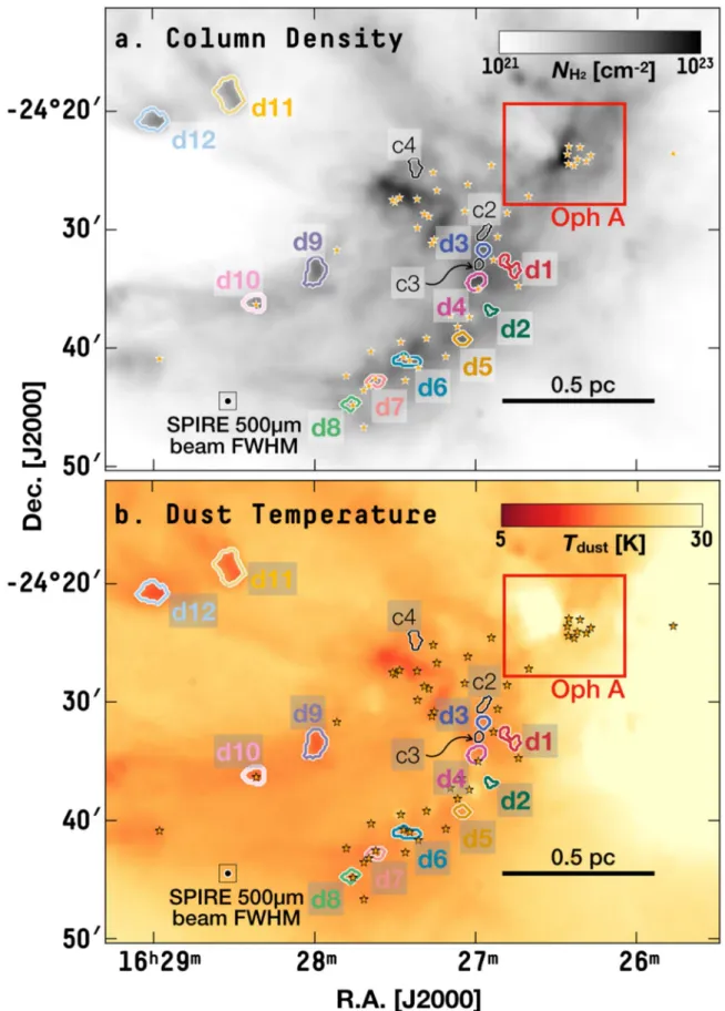
onto the same projection and gridding (Nyquist-sampled). Resulting maps column density and dust temperature are shown in Figures5 and6for L1688 in Ophiuchus and B18 in Taurus, respectively.
2.3. Source Catalogs
To understand droplets in context, we need compilations of the physical properties of previously identified dense cores. Goodman et al.(1993) (see Section2.3.1) present a summary
of cores from the observational surveys described in Benson & Myers(1989) and Ladd et al. (1994). The cores in Goodman
et al.(1993) have low, nearly thermal velocity dispersions, and
some of them are known to be“coherent” based on an apparent abrupt spatial transition from supersonic (in OH and C18O) to subsonic(in NH3) velocity dispersion (Goodman et al.1998; Caselli et al.2002). We also include the coherent core in the B5
region in Perseus, as observed in NH3(Pineda et al.2010), the only coherent structure known before this work where the spatial change in line width is captured in a single tracer.
2.3.1. Dense Cores Measured in NH3
Goodman et al.(1993) presented a survey of 43 sources with
observations of NH3 line emission (see Tables 1 and 2 in Goodman et al. (1993); see also the SIMBAD object list20),
based on observations made by Benson & Myers (1989) and
Ladd et al. (1994). The observations were carried out at the
37 m telescope of the Haystack Observatory and the 43 m telescope of the National Radio Astronomy Observatory (NRAO), resulting in a spatial resolution coarser than the modern GBT observations by a factor of ∼2.5. The velocity resolution of observations done by Benson & Myers (1989)
and Ladd et al. (1994) ranges from 0.07 to 0.20 km s−1. For comparison with the kinematic properties of the droplets measured using the GAS observations of NH3 emission (Friesen et al.2017), we adopt values that were also measured
using observations of NH3 hyperfine line emission, presented by Goodman et al.(1993). We correct the physical properties
summarized in Goodman et al. (1993) with the modern
measurement of the distance to each region. The updated distances are summarized in AppendixA.
The updated distances affect the physical properties listed in Table 1 in Goodman et al. (1998). The size scales with the
distance, D, by a linear relation, Rµ . Because the mass wasD
calculated from the number density derived from NH3 hyperfine line fitting, it scales with the volume of the structure—and thus M∝D3. The updated distances also affect the velocity gradient and related quantities listed in Tables 1 and 2 in Goodman et al.(1998), which we do not use for the
analyses presented in this work.
Apart from the updated distances, we combine the measure-ments of the kinetic temperature and the NH3 line width, originally presented by Benson & Myers(1989) and Ladd et al.
(1994), to derive the thermal and the nonthermal components
of the velocity dispersion. See Equation (1) below for the
definitions of the velocity dispersion components.
Among the 43 sources examined by Goodman et al. (1993),
eight sources were later confirmed by Goodman et al. (1998) and/
or Caselli et al.(2002) to be “coherent cores,” using a combination
of gas tracers of various critical densities(OH, C18O, NH3, and 19
In this paper, we use the mean molecular weight per H2molecule(2.8 u;mH2 in Kauffmann et al.(2008)) in the calculation of the mass and other
density-related quantities, and we use the mean molecular weight per free particle (2.37 u; μp in Kauffmann et al. (2008)) in the calculation of the velocity dispersion and pressure. Both numbers are derived assuming a hydrogen mass ratio of MH/Mtotal≈0.71, a helium mass ratio of MHe/Mtotal≈0.27, and a metal mass ratio of MZ/Mtotal≈0.02 (Cox & Pilachowski 2000). See Appendix A.1 in Kauffmann et al.(2008).
20
http://simbad.harvard.edu/simbad/sim-ref?querymethod=bib&simbo= on&submit=submit+bibcode&bibcode=1993ApJ...406..528G
Figure 1.L1688 in Ophiuchus. Shown here are maps of(a) peak NH3(1, 1) brightness in the unit of main-beam temperature, Tpeak, and(b) kinetic temperature, Tkin. The colored contours mark the boundaries of droplets, and the black contours mark the boundaries of droplet candidates. Because L1688-c1E and L1688-c1W overlap with L1688-d1, they are not shown in thisfigure or Figure2(see Section3.1). The stars mark the positions of Class 0/I and flat-spectrum protostars from Dunham
et al.(2015). The scale bar at the bottom right corner corresponds to 0.5 pc at the distance of Ophiuchus. The black circle at the bottom-left corner of each panel shows
the beam FWHM of the GBT observations at 23 GHz. See AppendixBfor a gallery of the close-up views of the droplets.
4
N2H+). The interiors of these eight sources show signs of a uniform and nearly thermal distribution of velocity dispersion. However, unlike B5 and the newly identified coherent structures in this paper, the “transition to coherence” was not spatially
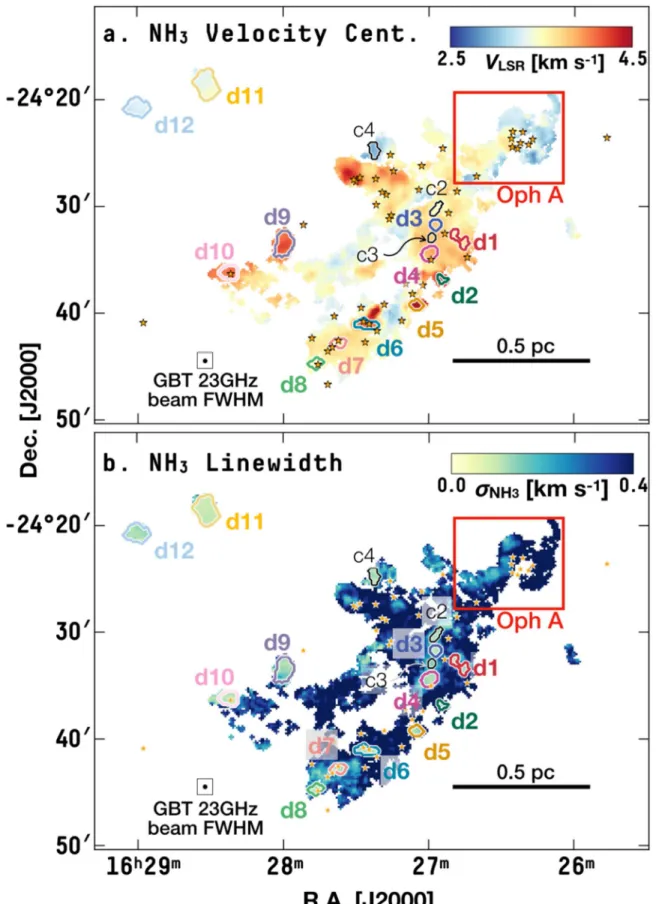
resolved with a single tracer for these eight coherent cores. For the ease of discussion, we refer to the entire sample of 43 sources as the“dense cores,” as they were originally referred to by Goodman et al. (1993). However, note that some of the 43 sources have Figure 2.Like Figure1, but for maps of(a) velocity centroid, VLSR, and(b) velocity dispersion,sNH3.
masses and sizes up to∼100 M☉and∼1 pc, respectively. These larger-scale structures do not strictlyfit in the definition of a dense core (with a small size and a nearly thermal velocity dispersion; see Section 4.3 for further discussion) and might be better categorized as“dense clumps” (as in McKee & Ostriker (2007)).
2.3.2. Coherent Core in B5
Using GBT observations of NH3 hyperfine line emission with a setup similar to GAS, Pineda et al. (2010) observed a
coherent core in the B5 region in Perseus and spatially resolved the“transition to coherence”—NH3line widths changing from supersonic values outside the core to subsonic values inside— for the first time. The coherent core sits in the eastern part of the molecular cloud in Perseus, at a distance of 315±32 pc (the quantities measured by Pineda et al. (2010) assuming a
distance of 250 pc are updated according to the new distance measurement; see Schlafly et al. (2014)). At 315 pc, the GBT
resolution at 23 GHz corresponds to a spatial resolution of ∼0.05 pc. The coherent core has an elongated shape, with a size of ∼0.2 pc.
Pineda et al. (2010) identified the coherent core in B5 as a
peak in NH3brightness surrounded by an abrupt change in NH3 velocity dispersion (∼4 km s−1pc−1). In the following analy-sis, we search the new GAS data for coherent structures reminiscent of the B5 core, looking for abrupt drops in NH3 line width to nearly thermal values around local concentrations of dense gas traced by NH3(see Section3.1for details). Below,
in the comparison between B5 and the newly identified coherent structures, we consistently follow the same methods adopted by Pineda et al. (2010) to derive the basic physical
properties using GBT observations of NH3 hyperfine line emission and Herschel column density maps derived from SED fitting (Section 2.2; see also Section 3.2 for details on the measurements of the physical properties).
3. Analysis
3.1. Identification of the Droplets
In this work, we look for coherent structures defined by abrupt drops in NH3line width and an interior with uniform, nearly thermal velocity dispersion,21reminiscent of previously known coherent cores examined by Goodman et al. (1998),
Caselli et al.(2002), and Pineda et al. (2010). We identify the
coherent structures using data from the GAS(see Section 2.1 Friesen et al.2017) and the Herschel maps of column density
and dust temperature derived in Section2.2, in order to enable a statistical analysis of coherent structures in two of the closest molecular clouds, Ophiuchus and Taurus.
With only the naked eye, one can already recognize many small plateaus of subsonic velocity dispersion associated with NH3-bright structures throughout L1688 and B18 in the maps
Figure 3.Like Figure1, but for B18 in Taurus, showing maps of(a) peak NH3(1, 1) brightness in the unit of main-beam temperature, Tpeak, and(b) kinetic temperature, Tkin. Here, the stars mark the positions of Class 0/I and flat-spectrum protostars with a reliability grade of A- or higher from Rebull et al. (2010). The scale bar at the bottom right corner corresponds to 0.5 pc at the distance of Taurus.
21
The data and the codes used for the analyses presented in this work are made public on GitHub at the repository: hopehhchen/Droplets (https:// github.com/hopehhchen/Droplets/tree/master/Droplets/).
6
of observed velocity dispersion (sNH3) and NH3 brightness
(Figures1–4). In order to quantitatively identify these coherent
structures, we follow the procedure adopted by Pineda et al. (2010) to identify the coherent core region in B5. The set of
criteria we use in this work to define the boundaries of coherent structures starts with the transition in velocity dispersion,sNH3,
from a supersonic to a subsonic value, and continues with the spatial distribution of NH3brightness, Tpeak, and the velocity centroid, VLSR. A set of quantitative prescriptions for defining the boundary of a coherent structure is given below as a step-by-step procedure:
1. We start with the intersection of areas enclosed by two contours: one of the NH3velocity dispersion and one of the NH3brightness. First, we find the contour where the NH3velocity dispersion (sNH3) has a nonthermal
comp-onent equal to the thermal compcomp-onent at the median kinetic temperature measured in the targeted region.(See Section 3.2and Equation(1) for details on the definition
of velocity dispersion components.) Second, we select the contour that corresponds to the 10σ level, where the NH3 brightness(Tpeak) is equal to 10 times the local rms noise, to match the extents of the contiguous regions where successful fits to the NH3 (1, 1) profiles were found in Friesen et al. (2017). The intersection of the areas
enclosed by these two contours is then used to define an initial mask. By this definition, the initial mask encloses a region where we have subsonic velocity dispersion and a signal-to-noise ratio greater than 10.
2. We expect the pixels within the mask defined in Step 1 to have a continuous distribution of velocity centroids (VLSR). In this step, we remove pixels with VLSR that leads to local velocity gradients (between the targeted pixel and its neighboring pixels within the mask) larger than the overall velocity gradient found for all pixels within the mask by a factor of ∼2. This procedure generally removes pixels with local velocity gradients greater than 20–30 km s−1pc−1, which is larger than the velocity gradients known to exist because of realistic physical processes in these regions. The mask editing is done with the aid of Glue.22
3. We then check whether the mask from Step 2 contains a single local peak in NH3brightness. If there is more than one NH3brightness peak, wefind the contour level that corresponds to the saddle point between the peaks. This contour level is then used to separate the mask from Step 2 into regions, each of which has a single NH3brightness peak. However, if a region has an NH3brightness peak no more than three times the local rms noise level above the saddle point, the region is excluded, and only its sibling region with the brighter peak is kept. We examine and categorize the regions excluded in this step as candidates(see below).
Figure 4.Like Figure3but for maps of(a) velocity centroid, VLSR, and(b) velocity dispersion,sNH3.
22
A GUI Python library built to explore relationships within and among related data sets, including image arrays(Beaumont et al.2015; Robitaille et al.
4. The Herschel maps of column density and dust temperature are then used to make sure that the defined structure (a region from Step 3) is centered around a
local rise in column density and a dip in dust temperature, consistent with the expectation of dense cores(Crapsi et al.2007).
Figure 5.Like Figure1, but for maps of(a) total column density, NH2, and(b) dust temperature, Tdust, derived from Herschel observations.
8
5. Finally, we make sure that the resulting structure is resolved by the GBT beam at 23 GHz (32″). We impose two criteria:(1) the projected area needs to be larger than a beam, and(2) the effective radius (the geometric mean of the major and minor axes; see Section3.2) needs to be
larger than the beam FWHM.
Using these criteria, we identify 12 coherent structures in L1688 and six coherent structures in B18. In Figures 1–6, the boundaries of the identified coherent structures in L1688 and B18 are shown as colored contours. Although the criteria are consistent with those used by Pineda et al. (2010) to define
the coherent core in B5 and do not impose any limits on size, the newly identified coherent structures in L1688 and B18 are generally smaller than previously known coherent cores (see Section3.2). As mentioned in Section1, we refer to the newly identified coherent structures as “droplets” for ease of discussion.
As the criteria indicate, each droplet has a high NH3peak brightness and a subsonic velocity dispersion—in contrast to the ambient region, where if NH3emission is detected, wefind a mostly supersonic velocity dispersion and a moderate distribution of NH3brightness. Figure7shows the distributions of NH3 line widths and peak NH3 brightness in main-beam units, for all pixels where there is significant detection of NH3 emission and for pixels within the droplet boundaries (for the criteria used to determine the significance of detection, see Friesen et al. (2017)). We observe an overall anticorrelation
between the observed NH3line width and NH3brightness, and the relation between the two quantitiesflattens toward the high
NH3 brightness end when the NH3 line width approaches a thermally dominated value. The droplets are found in this regime of high NH3brightness and thermally dominated NH3 line widths.
Figure8shows the radial profile of NH3velocity dispersion; the virtually constant NH3velocity dispersion in the interiors is consistent with what Goodman et al.(1998) found for coherent
cores (see also Pineda et al. 2010). See Appendix B for a gallery of the close-up views of the droplets.
Two of the 18 droplets, L1688-d11 and B18-d4, are found at the positions of the dense cores analyzed by Goodman et al. (1993), L1696A and TMC-2A, respectively. The two droplets
correspond to the central parts of the corresponding dense cores and have radii a factor of∼0.7 times the radii measured for these dense cores (Benson & Myers 1989; Goodman et al.
1993; Ladd et al.1994). See AppendixCfor a comparison of measured properties.
In Figures1–6, we also plot the positions of Class 0/I and flat spectrum protostars in the catalogs presented by Dunham et al. (2015) and Rebull et al. (2010), for L1688 and B18,
respectively. Within the boundaries of six(out of 18) droplets —L1688-d4, L1688-d6, L1688-d7, L1688-d8, L1688-d10, and B18-d6—we find at least one protostar along the line of sight. Consistent with the results presented by Seo et al.(2015) and
Friesen et al. (2009), none of the six droplets where we find
protostar(s) within the boundaries show a strong signature of increased Tkin or sNH3 around the protostar(s). While the
existence of young stellar objects(YSOs) within the boundary of a droplet in the plane of the sky does not necessarily indicate actual associations of these six droplets with protostars, it is
Figure 8.NH3velocity dispersion as a function of distance from the center of each droplet. The dark green dots represent individual pixels inside the boundary of each droplet. The transparent green band shows the 1σ distribution of pixels in each distance bin, with a bin size equal to the beam FWHM of GAS observations. The dashed and dotted lines show the expected NH3line widths when the velocity dispersion nonthermal component is equal to the sonic speed and half the sonic speed, respectively. The vertical black line marks the effective radius, Reff, and the gray vertical band marks the uncertainty in Reff. A red asterisk indicates that the droplet has an elongated shape with an aspect ratio larger than 2 that could bias the measurements using equidistant annuli(L1688-d1, L1688-d6, and B18-d5), and a blue asterisk indicates that the droplet sits near the edge of the region where NH3emission is detected, resulting in the measurements at larger radii being dominated by fewer pixels (L1688-d2 and L1688-d5).
Figure 7.Distributions of NH3line widths and peak NH3brightness in main-beam units, for every pixel with significant detection of NH3(1, 1) emission (a) in L1688 and(b) in B18. The 2D histogram in each panel shows the distribution of pixels in the entire map, with the pixel frequency defined as the percentage of pixels on the map falling in each 2D bin in the 2D histogram. The colored dots are individual pixels inside droplets, with colors matching the contours in Figures1,2, and5for L1688, and Figures3,4, and6for B18. The horizontal lines are the expected NH3line widths when the nonthermal component of velocity dispersion is respectively equal to the sonic speed(thicker line) and half the sonic speed (thinner line), for a medium with an average particle mass of 2.37 u and a temperature of 10 K.
10
possible that some of the droplets are associated with at least one YSO. See Section 4.3 for more discussion on the association between cores and YSOs and how it might be used as a way to define subsets of cores.
3.1.1. Droplet Candidates
Apart from the total of 18 droplets identified in L1688 and B18, we also includefive droplet candidates in L1688 (black contours in Figures 1, 2, and 5). Each droplet candidate is
identified by a spatial change from supersonic velocity dispersion outside the boundary to subsonic velocity dispersion inside. However, they do not meet at least one criterion listed above. The detailed reasons why each of these coherent structures is identified as a droplet candidate, instead of a droplet, are listed below:
1. L1688-c1E and L1688-c1W: These two droplet candi-dates are the eastern and western parts of the droplet L1688-d1, each of which has a local peak in NH3 brightness. However, neither peak is more than three times the local rms noise level above the saddle point between them, i.e., neither satisfies the criterion described in Step 3. Thus, we identify the entire region as a single droplet, L1688-d1, and include the eastern and the western parts of L1688-d1 as two droplet candidates. 2. L1688-c2: This droplet candidate shows a local dip in
NH3 velocity dispersion and a local peak in NH3 brightness. However, the local peak in NH3 brightness cannot be separated from the emission in the droplet L1688-d3 by more than three times the local rms noise in NH3(1, 1) observations, nor do we find an independent local peak corresponding to L1688-c2 on the Herschel column density map. (That is, L1688-c2 does not meet the criteria described in Steps 3 and 4 above.)
3. L1688-c3: Similar to L1688-c2, L1688-c3 shows a local dip in NH3velocity dispersion and a local peak in NH3 brightness. However, the local peak in NH3 brightness cannot be separated from the emission in the droplet L1688-d4 by more than three times the local rms noise in NH3(1, 1) observations, nor do we find an independent local peak corresponding to L1688-c3 on the Herschel column density map. While the projected area of L1688-c3 is larger than a beam, its effective radius is only∼2.6 times the beam FWHM.(That is, L1688-c3 does not meet the criteria described in Steps 3–5 above.)
4. L1688-c4: While L1688-c4 does show a significant dip in NH3velocity dispersion and an independent peak in NH3 brightness, it sits close to the edge of the region where the signal-to-noise ratio of the NH3 (1, 1) emission is sufficient for us to obtain a confident fit to the hyperfine line profile (Friesen et al.2017). We do not find a strong
and independent local peak corresponding to L1688-c4 on the Herschel column density map, either. Thus, we classify L1688-c4 as a droplet candidate.(That is, L1688-c4 does not meet the criterion described in Step 4 above.) In the following analyses, when we discuss the properties of the droplets—or, together with previously known coherent cores, the coherent structures—we exclude the droplet candidates. The droplet candidates are included on the plots to show the distributions of physical properties of potential coherent structures at even smaller scales, which are only marginally resolved by the GAS observations. The Oph A region (marked by the red
rectangles in Figures 1, 2, and 5) could potentially host more
droplets/droplet candidates. However, Oph A is known to also host a cluster of YSOs—and as Figures2(b) and5(b) show, the
extent of cold and subsonic dense gas identifiable on the maps of dust temperature and NH3 velocity dispersion is limited. No coherent structure that satisfies the above criteria can be identified. The same methods devised here to identify the boundaries and derive the physical properties of the coherent structures in L1688 and in B18 are applied on the data obtained by Pineda et al. (2010) to derive the physical properties of the coherent
core in Perseus B5 in the following analyses. 3.1.2. Contrast with Velocity Coherent Filaments
We note that Hacar et al.(2013) and Tafalla & Hacar (2015)
used the term“coherent” to describe continuous structures in the position–position–velocity space, with continuous distributions of line-of-sight velocity (VLSR). The method they adopted is a friend-of-friend clustering algorithm and does not impose any criteria on the velocity dispersion. In Step 2, we require a coherent structure to have a continuous distribution of VLSR; ergo, the newly identified coherent structures could theoretically be parts of“velocity coherent filaments.” However, the same can be said of any structures that are identified to have continuous structures on the plane of the sky and continuous distributions of line-of-sight velocity. We do not recommend equating the coherent structures, including the newly identified droplets in this work and the coherent cores previously analyzed by Goodman et al.(1998), Caselli et al. (2002), and Pineda et al.
(2010), to “velocity coherent filaments” identified by Hacar et al.
(2013). Specifically, the droplets and other coherent structures
are defined by abrupt drops in velocity dispersion from supersonic to subsonic values around their boundaries, which none of the “velocity coherent filaments” examined by Hacar et al.(2013) show. Moreover, in contrast to the elongated shapes
of the “velocity coherent filaments” examined by Hacar et al. (2013), the droplets are mostly round, with aspect ratios
generally between 1 and 2. (There are three exceptions: L1688-d1, with an aspect ratio of ∼2.50; L1688-d6, with an aspect ratio of∼2.52; and B18-d5, with an aspect ratio of ∼2.03. These exceptions are marked with red asterisks on Figure8).
3.2. Mass, Size, and Velocity Dispersion
With the droplet boundary defined in Section 3.1, we calculate the mass of each droplet using the column density map derived from SED fitting of Herschel observations (see Section 2.2). To remove the contribution of line-of-sight
material, the minimum column density within the droplet boundary is used as a baseline and subtracted off. The mass is then estimated by summing column density (after baseline subtraction) within the droplet boundary. This baseline subtraction method is similar to the “clipping paradigm” studied by Rosolowsky et al.(2008b), and has been applied by
Pineda et al. (2015) to estimate the mass of structures within
the coherent core in B5. For the droplets, we find a typical mass23of 0.4-+0.30.4M☉. Table1lists the mass of each droplet. In AppendixE, we discuss the reasons for adopting the clipping
23
Unless otherwise noted, the typical value of each physical property presented in this work is the median value of the entire sample of 18 droplets— excluding the droplet candidates—with the upper and lower bounds being the values measured at the 84th and 16th percentiles, which would correspond to±1 standard deviation around the median value if the distribution is Gaussian.
Table 1
Physical Properties of Droplets and Droplet Candidates
IDa Position Massb Effective Radiusc NH
3Line Widthd NH3Kinetic Temp. Total Vel. Dispersione YSO(s)f
[J2000] (M) (R
eff) (sNH3) (Tkin) (s )tot
R.A. Decl. (M☉) (pc) (km s−1) (K) (km s−1) L1688-d1 16h26m47 07 −24°33′8 3 0.17±0.03 0.038-+0.0310.007 0.14±0.01 12.0±0.6 0.24±0.01 N L1688-d2 16h26m54 54 −24°36′52 4 0.03±0.01 0.020-+0.0080.007 0.16±0.01 12.8±0.9 0.25±0.01 N L1688-d3 16h26m57 07 −24°31′44 8 0.08±0.03 0.024 0.0070.007 -+ 0.12±0.01 10.2±0.3 0.21±0.01 N L1688-d4 16h26m59 59 −24°34′28 8 0.73±0.05 0.033-+0.0070.007 0.14±0.01 10.6±0.2 0.23±0.01 Y L1688-d5 16h27m4 96 −24°39′17 6 0.13±0.03 0.025-+0.0070.007 0.14±0.01 12.4±0.6 0.24±0.01 N L1688-d6 16h27m25 50 −24°41′6 2 0.22±0.04 0.032 0.0110.018 -+ 0.12±0.01 12.6±0.4 0.23±0.01 Y L1688-d7 16h27m37 27 −24°42′50 2 0.10±0.02 0.026-+0.0070.009 0.13±0.01 13.2±0.4 0.24±0.01 Y L1688-d8 16h27m46 44 −24°44′45 4 0.10±0.01 0.026-+0.0070.009 0.13±0.01 12.7±0.7 0.23±0.01 Y L1688-d9 16h27m59 43 −24°33′33 0 0.55±0.03 0.043 0.0080.021 -+ 0.14±0.01 11.2±0.5 0.23±0.01 N L1688-d10 16h28m22 12 −24°36′16 8 0.22±0.02 0.034-+0.0070.009 0.11±0.01 11.5±0.5 0.22±0.01 Y L1688-d11 16h28m31 53 −24°18′36 1 0.46±0.02 0.054-+0.0120.010 0.10±0.01 10.1±0.8 0.20±0.01 N L1688-d12 16h28m59 99 −24°20′45 2 0.38±0.02 0.042 0.0070.014 -+ 0.12±0.01 10.1±0.5 0.21±0.01 N L1688-c1Eg 16h26m49 36 −24°32′39 0 0.02±0.02 0.020-+0.0070.007 0.14±0.01 12.4±0.7 0.24±0.01 N L1688-c1Wh 16h26m45 22 −24°33′30 5 0.07±0.02 0.022 0.0070.007 -+ 0.15±0.01 11.9±0.5 0.24±0.01 N L1688-c2 16h26m56 89 −24°30′18 7 0.10±0.02 0.024-+0.0100.011 0.12±0.01 11.3±0.4 0.22±0.01 N L1688-c3 16h26m58 74 −24°33′1 4 0.06±0.02 0.019-+0.0070.007 0.15±0.01 11.7±0.4 0.24±0.01 N L1688-c4 16h27m22 28 −24°24′52 2 0.05±0.02 0.028 0.007 0.007 -+ 0.12±0.01 12.8±0.9 0.23±0.01 N B18-d1 4h26m58 95 24°41′16 6 0.34±0.02 0.064 0.0250.027 -+ 0.09±0.01 10.5±1.2 0.20±0.01 N B18-d2 4h29m24 13 24°34′42 2 1.24±0.05 0.045 0.012 0.021 -+ 0.11±0.01 10.0±0.4 0.21±0.01 N B18-d3 4h30m5 71 24°25′40 6 0.49±0.02 0.044-+0.0070.014 0.08±0.01 9.8±0.9 0.19±0.01 N B18-d4 4h31m54 48 24°32′28 2 0.56±0.03 0.050 0.0240.022 -+ 0.11±0.01 9.1±0.3 0.20±0.01 N B18-d5 4h32m46 54 24°24′51 9 1.87±0.05 0.071-+0.0190.034 0.11±0.01 9.5±0.4 0.20±0.01 N B18-d6 4h35m36 32 24°9′0 7 0.72±0.04 0.048-+0.0220.017 0.13±0.01 9.9±0.3 0.22±0.01 Y Notes. a
L1688-c1E to L1688-c4 are droplet candidates.
bBased on the column density map derived from SEDfitting of Herschel observations. See Section2.2. c
The geometric mean of the Tpeakweighted spatial dispersions along the major and the minor axes. See Section3.2. See also AppendixDfor details on determining the uncertainties.
d
The best-fit Gaussian σ.
e
Derived from NH3line widths and kinetic temperatures. See Equation(1).
f
A value of“Y” means that there is at least one YSO within the droplet boundary defined on the plane of the sky (see Section3.1), and a value of “N” means that there is no YSO within the droplet boundary. The YSO positions are taken from the catalog presented by Rebull et al.(2010) for B18, and the catalog presented by Dunham et al. (2015) for L1688. Because we are interested in the association between cores/droplets and the YSOs potentially forming inside, only Class 0/I and flat spectrum protostars are considered here.
g
The eastern part of L1688-d1.
h
The western part of L1688-d1.
12 The Astrophysical Journal, 877:93 (42pp ), 2019 June 1 Chen et al.
method and the uncertainty therein, and in Appendix F, we examine the uncertainty in mass measurements due to the potential bias in SEDfitting.
We define the radius of each droplet based on the NH3 brightness–weighted second moments along the major and minor axes. We designate the major axis direction as the one with the greatest dispersion in Tpeak according to a principal component analysis (PCA), and the minor axis is oriented perpendicular to the major axis.24The effective radius is then the geometric mean of sizes along the major and minor axes,
Reff= rmaj minr , where rmaj and rmin are derived by multi-plying the NH3 brightness–weighted second moments by a factor of 2 2 ln 2 , the scaling factor between the second moment and the FWHM for a Gaussian shape. The multi-plication of the scaling factor of2 2 ln 2 is done in the same way as the method applied by Benson & Myers (1989) and
Goodman et al.(1993) to estimate the radii of dense cores, and
is applied to approximate the“true radius” of the droplet. The resulting effective radii of droplets are listed in Table1
and have a typical value of 0.04±0.01 pc. The effects of the resolution and the irregular shape of the boundary are included in the uncertainties listed in Table 1. Figure8 shows that the effective radius, Reff, plotted on top of the radial profile of velocity dispersion,sNH3, of each droplet, well-characterizes the
change from supersonic to subsonic velocity dispersion. See Appendix B for a comparison between a circle with a radius equal to Reffand the actual boundary of a droplet on the plane of the sky, and see Appendix Dfor details on estimating the uncertainty and for a discussion on other common ways to derive the“effective radius.”
From the GAS observations, we derive the NH3 velocity dispersion, sNH3, and the gas kinetic temperature, Tkin
(Figures 1–4; see Section 2.1.1 for details). Assuming that the bulk molecular component is in thermal equilibrium with the NH3 component and assuming also that the nonthermal component of the velocity dispersion is independent of the chemical species observed, we can estimate a total velocity dispersion, s , from the thermal component, σtot T, and the nonthermal (turbulent) component, σNT:
1 tot 2 NT 2 T 2 s =s +s ( ) k T m k T m , NH 2 B kin NH B kin ave 3 3 s =⎛ - + ⎝ ⎜ ⎞ ⎠ ⎟
where kBis the Boltzmann constant, and mNH3and maveare the
molecular weight of NH3 and the mean molecular weight in molecular clouds, respectively. Note that the thermal comp-onent, σT, is by definition equal to the sonic speed, cs, in a medium with a particle mass of maveat a temperature of Tkin. Following Kauffmann et al.(2008), we use the mean molecular
weight per free particle of 2.37 u(μpin Kauffmann et al.2008). For each droplet, we obtain characteristic values of the NH3 velocity dispersion,sNH3, and the kinetic temperature, Tkin, by
taking the median value for the pixels within the droplet boundary on the parameter maps. Following Equation (1), we
then estimateσNT,σT, andσtotfor each droplet. Note thatσtotis sometimes referred to as the “1D velocity dispersion,” concerning the motions along the line of sight, as opposed to
the“3D velocity dispersion,” which cannot be observed but can be estimated by multiplying the 1D velocity dispersion by a factor of 3 assuming isotropy. We find a typical σtot of 0.22±0.02 km s−1 for the droplets (see Table 1). For
reference, the purely thermal velocity dispersion at 10 K is 0.19 km s−1.
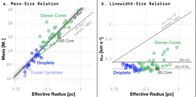
Figure 9 shows the distributions of mass, M, and total velocity dispersion, σtot, plotted against the effective radius, Reff, of droplets/droplet candidates in comparison with previously known coherent cores as well as other dense cores (see Section2.3for details on how the physical properties were estimated for the dense cores). Figure9(a) shows that droplets
seem to fall along the same mass–radius relation as the dense/ coherent cores. Using a gradient-based MCMC sampler tofind a power-law relation between the mass and effective radius,
M µReffp, for all the previously known dense/coherent cores (including B5) and the droplets (excluding droplet candidates), we find a power-law index, p=2.4±0.1.25 This exponent lies between those expected for structures with constant surface density, M∝R2, and those for structures with constant volume density, M∝R3. As a reference, Larson(1981) found a scaling
law, M∝R1.9, for larger-scale molecular structures(with sizes of 0.1–100 pc and masses of 1 M☉ to 3×10⁵M☉), using a compilation of observations of molecular line emission from species including 12CO, 13CO, H2CO, and for a few objects, NH3, and other N-bearing species.
Figure9(b) shows the relationship between σtotand Reff. At scales below 0.1 pc, all structures shown have a subsonic velocity dispersion. The continuity of the distribution of M, Reff, andσtotbetween the newly identified coherent structures (droplets) and the previously known coherent cores, as well as other dense cores, suggests that the identification of droplets is robust—and that droplets fall toward the smaller-size end of a potentially continuous population of coherent structures across different size scales. We discuss this continuity in detail, in Section4.3.
3.3. Virial Analysis: Kinetic Support, Self-gravity, and Ambient Gas Pressure
To investigate the stability of the coherent structures, we follow Pattle et al. (2015) to consider the balance between
internal kinetic energy, self-gravity, and the ambient gas pressure, with respect to the equilibrium expression:
2W = - W + WK ( G P) ( )2 whereΩKis the internal kinetic energy,ΩGis the gravitational potential energy, and ΩP is the energy term representing the confinement provided by the ambient gas pressure acting on the structure. The “external pressure” comes from thermal and nonthermal (turbulent) motions of the ambient gas (see the analysis in Section 3.3.3). Because we do not have the
observations needed to estimate magnetic energy, the magnetic energy term, ΩM, is omitted (compared to Equation (27) in Pattle et al.(2015)). Here, we focus on pressure exerted on a
structure by thermal and nonthermal(turbulent) motions of the ambient gas forΩP, and we ignore any contribution of ionizing photons to pressure(see discussions in Ward-Thompson et al. (2006) and Pattle et al. (2015)).
24
The same process is used to define the major and minor axes in the Python package for computing the dendrogram, astrodendro. See http://
dendrograms.org/for documentation.
25
The gradient-based MCMC sampling is implemented using the Python package, PyMC3. Seehttp://docs.pymc.io/index.htmlfor documentation.
3.3.1. Internal Kinetic Energy,ΩK
The internal kinetic energy, ΩK, is given by:
M 3 2 3 K tot 2 s W = ( )
where M is the mass and σtotis the total velocity dispersion, estimated from the observed NH3 velocity dispersion, sNH3,
and gas kinetic temperature, Tkin, following Equation(1) (see Section 3.2 for details). The factor of 3 stands for the correction applied to the “1D velocity dispersion,” σtot, to obtain an estimate of the 3D velocity dispersion, assuming isotropy(see Section3.2). For droplets, we measure a typical
kinetic energy of 4.5-+2.85.8´1041erg. Table2 gives results for each droplet.
3.3.2. Gravitational Potential Energy,ΩG
Assuming spherical geometry, gravitational potential energy, ΩG, can be estimated from total mass and an effective radius; we adopt a gravitational potential energy expression:
GM R 3 5 4 G 2 eff W = - ( )
where we assume that the sphere of material has a uniform density distribution. In comparison, a sphere of material with a power-law density distribution,ρ∝r−2, has an absolute value of gravitational potential energy,∣WG∣, a factor of∼1.7 larger
than that expressed in Equation (4), and a sphere with a
Gaussian density distribution has∣WG∣ a factor of ∼2 smaller
than that expressed in Equation (4) (Pattle et al. 2015; Kirk et al. 2017b). In the following analysis, we include the
deviation in ΩG due to different assumptions of density
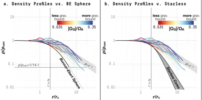
distributions in the estimated errors. In Section4.1.1, we show that the density distributions in droplets are nearly uniform at small radii with relatively shallow drops toward the outer edges, validating the assumption of a uniform density distribution used to derive Equation(4).
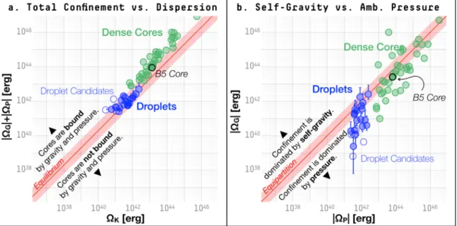
For droplets, we measure a typical gravitational potential energy of 1.3-+1.15.0´1041erg (absolute value; see Table 2). Figure 10(a) shows that most of the dense cores, including
previously known coherent cores such as the one in B5, are close to an equilibrium between the gravitational potential energy and the internal kinetic energy. This indicates that the self-gravity of these coherent cores is substantial and may provide the binding force needed to keep the cores from dispersing. On the other hand, gravity in the newly identified droplets appears to be less dominant compared to the internal kinetic energy. For most of the droplets, the internal kinetic energy is close to an order of magnitude larger than the gravitational potential energy.
That larger structures have more dominant gravitational potential energies than smaller structures is expected for structures with a nearly flat σtot-size relation and a steep mass–size relation (Figure9). For the coherent structures under
discussion, we observe a power-law mass–size relation,
M µReff2.4, and with a constant σtot, we would expect a power-law relation between the gravitational potential energy and the size,∣WG∣µReff3.8, and a power-law relation between
the internal kinetic energy and the size, K Reff 2.4
W µ .
Conse-quently, a smaller coherent structure would have a smaller ratio between the gravitational potential energy and the internal kinetic energy, ∣WG∣ WK. For reference, structures with a
constant∣WG∣ WKare expected to have a mass–size relation of
M∝Reff.
Figure 9.(a) Mass, M, plotted against the effective radius, Reff, for dense cores(green circles), the coherent core in B5 (a green circle marked with a black edge), and the newly identified coherent structures: droplets (filled blue circles) and droplet candidates (empty blue circles). The black line shows a power-law relation between the mass and the effective radius, found for both the dense cores(including B5) and the droplets (excluding droplet candidates) by a gradient-based MCMC sampler. A randomly selected 10% of the accepted parameters in the MCMC chain are plotted as transparent lines for reference. The solid gray line shows the empirical relation based on observations of larger-scale structures examined by Larson(1981). (b) The total velocity dispersion,s , plotted against the effective radius, Rtot eff, for the same structures as in(a). The horizontal lines shows expected for structures where the nonthermal component is equal to the sonic speed (ctot s; thicker line) and half the sonic speed(thinner line) of a medium with an mean molecular weight of 2.37 u at a temperature of 10 K. The gray line shows an empirical relation adopted from Larson(1981). Here, we convert the line width in the relation presented by Larson (1981) tos by assuming that the line width was measured from the CO (1–0) linetot emission with a gas temperature of 10 K.
14
The above comparison between the gravitational potential energy and the internal kinetic energy, without considering the ambient turbulent pressure, is analogous to an analysis of stability using a virial parameter, a R
GM
vir tot
2 eff
a = s , where the leading factor, a, varies according to the assumption of the density distribution(e.g., a = 5 for a spherical structure with a uniform density, and a= 3 for a spherical structure with a power-law density profile with an index of 2, ρ∝r−2; see Bertoldi & McKee (1992)). Conventionally, structures with
αvir2 would be considered “gravitationally bound.” By this measure, only the most massive droplets (with masses on the order of 1 M☉) along with most of the dense cores are “gravitationally bound” (Figure10(a)).
3.3.3. Energy Term Representing Ambient Pressure Confinement, ΩP
The pressure term,ΩP, in the virial equation(Equation (2)) is characteristic of the pressure exerted on a structure by thermal and nonthermal (turbulent) motions of the ambient gas. To avoid the impression that there is a clear-cut boundary between the interior and the exterior of the targeted structure, we call the pressure provided by the ambient gas motions the“ambient gas
pressure,” Pamb, which is sometimes called the “external pressure” and denoted by Pext in previous works (Ward-Thompson et al.2007; Pattle et al. 2015; Kirk et al.2017b).
For a spherical structure with a radius of Reff, the pressure term is given by
P V P R
3 4 , 5
P amb amb eff
3
p
W = - = - ( )
where Pambis the ambient gas pressure and V is the volume of the structure under discussion (Ward-Thompson et al. 2006; Pattle et al.2015). The pressure exerted on the structure can be
estimated from
Pamb amb tot,amb, 6
2
r s
= ( )
whereρambis the volume density of the ambient gas andstot,ambis
the total velocity dispersion, including both thermal and nonthermal motions of the ambient gas(same as σtot defined in Equation(1) for the gas in the core). The leading factor of 3 in
Equation(5) is applied to estimate the effects of gas motions in the
3D space, because for stot,amb, we use the “1D (line-of-sight)
Table 2
Virial Properties of Droplets and Droplet Candidates
IDa Internal Kinetic Energyb Gravitational Potential Energyc Ambient Gas Pressured Energy Term for Ambient Pressuree
(W )K (∣WG∣) (Pamb kB) (∣WP∣)
(erg) (erg) (K cm−3) (erg)
L1688-d1 2.90.5´1041 4.0 10 2.0 2.7´ 40 -+ 7.00.7´105 2.00.3´1042 L1688-d2 5.92.9´1040 2.4 10 2.4 1.6´ 39 -+ 8.41.3´105 3.30.6´1041 L1688-d3 1.00.4´1041 1.2 10 0.9 0.8´ 40 -+ 6.80.7´105 4.50.6´1041 L1688-d4 1.10.1´1042 8.3 10 4.1 5.5´ 41 -+ 6.70.8´105 1.20.2´1042 L1688-d5 2.20.5´1041 3.4 10 1.7 2.3´ 40 -+ 1.50.2´106 1.10.2´1042 L1688-d6 3.60.6´1041 8.1 10 4.1 5.4 ´ 40 -+ 9.71.4´105 1.60.3´1042 L1688-d7 1.80.3´1041 2.1 10 1.0 1.4 ´ 40 -+ 4.10.6´105 3.80.6´1041 L1688-d8 1.60.2´1041 1.9 10 0.91.3´ 40 -+ 2.70.4´105 2.40.4´1041 L1688-d9 8.50.6´1041 3.6 10 1.8 2.4´ 41 -+ 2.60.5´105 1.10.2´1042 L1688-d10 3.20.3´1041 7.7 10 3.8 5.1´ 40 -+ 2.80.5´105 5.41.0´1041 L1688-d11 5.50.5´1041 2.0 10 1.01.3´ 41 -+ 5.01.0´104 4.00.9´1041 L1688-d12 5.10.4´1041 1.7 10 0.9 1.1´ 41 -+ 9.71.3´104 3.80.6´1041 L1688-c1Ef 2.63.3´1040 6.5 10 6.5 4.3´ 38 -+ 7.70.8´105 3.10.4´1041 L1688-c1Wg 1.10.3´1041 1.1 10 0.6 0.7´ 40 -+ 7.80.8´105 4.10.6´1041 L1688-c2 1.50.3´1041 2.1 10 1.1 1.4 ´ 40 -+ 6.40.7´105 4.60.7´1041 L1688-c3 1.10.4´1041 1.2 10 0.9 0.8´ 40 -+ 7.90.8´105 2.60.4´1041 L1688-c4 7.83.0´1040 4.4 10 3.3 2.9´ 39 -+ 1.20.1´106 1.30.2´1042 B18-d1 3.90.5´1041 9.1 10 4.5 6.0 ´ 40 -+ 6.81.2´104 9.03.3´1041 B18-d2 1.50.1´1042 1.8 10 0.9 1.2´ 42 -+ 1.80.3´105 8.23.0´1041 B18-d3 5.40.5´1041 2.8 10 1.4 1.9´ 41 -+ 1.20.1´105 5.21.7´1041 B18-d4 6.50.4´1041 3.3 10 1.6 2.2´ 41 -+ 6.60.9´104 4.21.4´1041 B18-d5 2.30.1´1042 2.5 10 1.3 1.7´ 42 -+ 1.40.3´105 2.51.0´1042 B18-d6 1.00.1´1042 5.5 10 2.8 3.7´ 41 -+ 1.80.4´105 1.00.4´1042 Notes. a
L1688-c1E to L1688-c4 are droplet candidates. b
See Equation(3). c
A potential energy, with the zero point defined at infinity. The effects of various assumptions regarding the geometry are considered in error estimation. Absolute values are listed in this table. See Equation(4) and the text.
d
Measured in the region immediately outside each droplet. See Equation(6). e
A potential energy, with the zero point defined at equilibrium. Absolute values are listed in this table. See Equation (5). f
The eastern part of L1688-d1. g
velocity dispersion” measured from observations. See the discussion in Section3.2.
We base our calculation of the pressure, Pamb, on the maps of
NH3
s and Tkin from fitting the NH3hyperfine line profiles (for estimatingstot,amb;Figures1–4) and the Herschel column density maps (for estimating ramb; Figures 5 and 6). The former is possible because there is significant detection of NH3 (1, 1) emission in regions surrounding the droplets and the coherent core in B5, which appear embedded in the dense gas components
of the clouds(see Figures2 and4). We use the region (on the
plane of the sky) immediately outside the targeted structure but within R( eff +0.1) pc from the center of the structure to obtain an estimate of the ambient gas pressure. Because the typical sonic scale in nearby molecular clouds is roughly 0.1 pc (Federrath
2013), our hope is that the selected region represents the
projection of the volume within a sonic scale from the surface of the structure and that the estimated pressure is from the motions of the gas relevant in confining the structure. The volume density
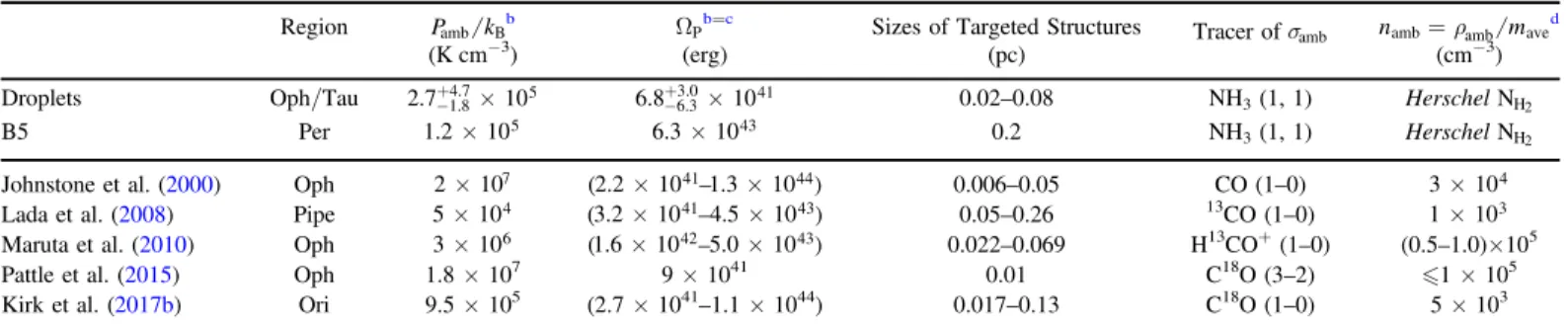
Table 3
External Pressure of Droplets Compared to Previous Worksa
Region Pamb kBb WPb=c Sizes of Targeted Structures Tracer ofsamb namb=ramb maved
(K cm−3) (erg) (pc) (cm−3)
Droplets Oph/Tau 2.7-+1.84.7´105 6.8-+6.33.0´1041 0.02–0.08 NH3(1, 1) Herschel NH2
B5 Per 1.2´105 6.3´1043 0.2 NH
3(1, 1) Herschel NH2 Johnstone et al.(2000) Oph 2´107 (2.2´1041–1.3´1044) 0.006–0.05 CO(1–0) 3´104 Lada et al.(2008) Pipe 5´104 (3.2´1041–4.5´1043) 0.05–0.26 13
CO(1–0) 1´103 Maruta et al.(2010) Oph 3´106 (1.6´1042–5.0´1043) 0.022–0.069 H13
CO+(1–0) (0.5–1.0)×105 Pattle et al.(2015) Oph 1.8×10⁷ 9×1041 0.01 C18O(3–2) 1×10⁵ Kirk et al.(2017b) Ori 9.5×10⁵ (2.7×1041–1.1×1044) 0.017–0.13 C18O(1–0) 5×10³ Notes.
a
This table compares estimates of the ambient pressure and the corresponding virial energy term presented in Section3.3.3with previous estimates for other density structures found in molecular clouds. We only include estimates based on direct observations of the velocity dispersion of the ambient material in this table, and it is by no means meant to be comprehensive. Other efforts to estimate the ambient pressure include the work presented by Seo et al.(2015), where estimates are made by
modeling the surface pressure using measurements at the peripheries of cores, and that presented by Fischera & Martin(2012), where estimates are made for
filamentary structures based on surface brightness models of near-equilibrium cylinders, for example. See discussion in Section3.3.3. b
The pressure due to the thermal and nonthermal motions of the gas surrounding the targeted structures. See Section3.3.3for details. c
The energy term is calculated according to Equation(5). Numbers in parentheses are not reported by the original authors and are instead derived here based on the
ambient gas pressures and the radii of corresponding structures. d
For each of the droplets and the coherent core in B5, the density of the ambient gas is estimated based on the Herschel column density map. Other works derived the ambient gas density by assuming a“critical density” that the velocity dispersion tracer traces. The number density assumed to be traced by the ambient gas tracer is listed for reference.
Figure 10.(a) Gravitational potential energy,W , plotted against internal kinetic energy,G W , for dense cores (green circles), the coherent core in B5 (a green circleK marked with a black edge), and the newly identified coherent structures: droplets (filled blue circles) and droplet candidates (empty blue circles). The red band from the lower left to the top right marks the equilibrium betweenW andG W (solid red line) within an order of magnitude (pink band). The black line marks where theK conventional virial parameter,a , has a value of 2. (b) The energy term representing the confinement provided by the ambient gas pressure,vir W , plotted against theP internal kinetic energy,W , for the same structures shown in (a). Similarly, the red band from the lower left to the top right marks an equilibrium betweenK W andP WK (solid red line) within an order of magnitude (pink red band).
16