Analysis of a supercritical hydrogen liquefaction cycle

Analysis of a Supercritical Hydrogen Liquefaction Cycle

by

Wayne Lawrence Staats, Jr.

B.S., Mechanical Engineering

University of Wisconsin-Madison, 2006

Submitted to the Department of Mechanical Engineering in partial fulfillment of the

requirements for the degree of Master of Science in Mechanical Engineering

at the

Massachusetts Institute of Technology

June, 2008

© 2008 Massachusetts Institute of Technology

All rights reserved

Signature of Author:

______________________________________________________

Department of Mechanical Engineering

May 27, 2008

Certified

by:

______________________________________________________

John G. Brisson

Professor of Mechanical Engineering

Thesis Supervisor

Accepted

by:

______________________________________________________

Lallit Anand

Chairman, Department Committee on Graduate Students

Analysis of a Supercritical Hydrogen Liquefaction Cycle by

Wayne Lawrence Staats, Jr.

Submitted to the Department of Mechanical Engineering on May 27, 2008 in partial fulfillment of the requirements for the degree of Master of Science in Mechanical Engineering

ABSTRACT

In this work, a supercritical hydrogen liquefaction cycle is proposed and analyzed numerically. If hydrogen is to be used as an energy carrier, the efficiency of liquefaction will become increasingly important. By examining some difficulties of commonly used industrial liquefaction cycles, several changes were suggested and a readily scalable, supercritical, helium-cooled hydrogen liquefaction cycle was proposed. A novel overlap in flow paths of the two coldest stages allowed the heat exchanger losses to be minimized and the use of a single-phase liquid expander eliminated the pressure reduction losses associated with a Joule-Thomson valve. A simulation program was written in MATLAB to investigate the effects of altering component efficiencies and various system parameters on the cycle efficiency.

In addition to performing the overall cycle simulations, several of the system components were studied in greater detail. First, the required volume of the ortho-para catalyst beds was estimated based on published experimental data. Next, the improvement in cycle efficiency due to the use of a single-phase liquid expander to reduce the pressure of the hydrogen stream was estimated. Finally, a heat exchanger simulation program was developed to verify the feasibility and to estimate the approximate size of the heat exchangers in the cycle simulation.

For a large, 50-ton-per-day plant with reasonable estimates of achievable component efficiencies, the proposed cycle offered a modest improvement in efficiency over the current state of the art. In comparison to the 30-40% Second Law efficiencies of today’s most advanced industrial plants, efficiencies of 39-44% were predicted for the proposed cycle, depending on the heat exchange area employed.

Thesis Supervisor: John G. Brisson Title: Professor of Mechanical Engineering

Acknowledgements

First, I thank Professor Brisson for his guidance and advice. I have learned a great deal working with him and he has always been available and helpful. Second, I am very appreciative of Professor Smith’s assistance in this project. My discussions with Professor Brisson and Professor Smith have been educational, thought-provoking and memorable.

I thank Gas Equipment Engineering Corporation (GEECO) for providing funding for this research. I have enjoyed working with Martin Shimko of GEECO.

My fellow Cryogenic Engineering Laboratory graduate students (Gunaranjan Chaudhry, Rory Monaghan, Teresa Baker, Fritz Pierre, Malima Wolf, David Lopez, Barbara Botros, and Martin Segado) have provided valuable conversation, advice and camaraderie. I have appreciated Doris Elsemiller’s astute administrative advice.

I am grateful to my parents and sisters for their continuing love, encouragement and friendship. Above all, my sincere thanks are due to my fiancée Brooke, who has been my greatest source of support and strength throughout this research.

Table of Contents

1.2.1. Orthohydrogen and parahydrogen ... 14

1.2.2. Ortho-para catalysts ... 18

1.2.3. Property differences between ortho and para... 19

1.2.4. Ideal work of liquefaction... 22

1.3. Hydrogen liquefaction plants... 25

1.3.1. Basic hydrogen liquefaction cycles ... 26

1.3.2. Previous and current plants... 27

1.3.3. Challenges of hydrogen liquefaction ... 30

CHAPTER 2. CYCLE SIMULATIONS ... 34

2.1. Design goals and component feasibility... 34

2.2. Proposed cycle... 37

2.3. Numerical simulations... 40

2.3.1. Spreadsheet-based... 40

2.3.2. Program-based ... 44

CHAPTER 3. COMPONENT SIMULATIONS ... 52

3.1. Catalyst beds... 52

3.2. Single-phase wet expander ... 58

3.3. Heat exchangers... 63

3.3.1. Single heat exchanger ... 63

3.3.2. Heat exchange area ... 67

CHAPTER 4. SUMMARY... 70

References... 72

Appendix A: Supplemental Plots... 77

Appendix B: MATLAB Code... 80

B1. cycle.m ... 80 B2. optimize.m ... 88 B3. para.m ... 92 B4. H2props.m ... 93 B5. expander.m ... 95 B6. HXode.m ... 96 B7. whatisUA.m... 100 B8. wet_expander_performance.m ... 102

List of Figures

Figure 1: Energy density of hydrogen as liquid and as compressed gas... 12 Figure 2: Equilibrium parahydrogen concentration vs. temperature [20]... 15 Figure 3: Mass fraction remaining and parahydrogen content for a completely adiabatic,

vented, constant pressure container of liquid hydrogen, as a function of time. ... 17 Figure 4: Ideal gas isobaric specific heat for parahydrogen, normal hydrogen and

orthohydrogen. The circles indicate the original, tabulated data from [20]. ... 20 Figure 5: A stream of hydrogen cooled by a reversible cyclic device. ... 24 Figure 6: Ideal work vs. temperature for gaseous equilibrium hydrogen. Also shown is

the ideal work of ortho-para conversion, which was determined by subtracting the ideal work to cool gaseous normal hydrogen from the ideal work to cool gaseous equilibrium hydrogen. ... 25 Figure 7: A simple Claude cycle [41]. ... 27 Figure 8: A dual pressure Claude cycle [41]... 28 Figure 9: Second Law efficiency versus capacity for cryogenic refrigerators and

liquefiers surveyed in 1974 [15]... 31 Figure 10: Ideal work of liquefaction vs. inlet hydrogen pressure, for a final state of 20 K,

1 bar and 95% parahydrogen... 35 Figure 11: Specific heat of equilibrium hydrogen vs. temperature at various pressures. ... 37 Figure 12: Schematic of the proposed system. ... 39 Figure 13: A two-stage, helium-cooled hydrogen liquefaction cycle that is typical of the

systems simulated... 41 Figure 14: Graphical output of the spreadsheet-based solver for the two-expander system.

Figure 15: Results of pilot plant cycle simulation. ... 48

Figure 16: Change in pilot plant system efficiency vs. change in component efficiency, with respect to the base configuration. All of the points coincide at the center which represents the base configuration. The components corresponding to the steeper lines affect the system efficiency most significantly. The parameters were varied from the base configuration one at a time... 49

Figure 17: Effect of helium compressor efficiency on cycle efficiency for the pilot plant. ... 50

Figure 18: Effect of hydrogen pressure on cycle efficiency for the pilot plant. ... 51

Figure 19: Estimation of the mass transfer conductance from experimental data. ... 54

Figure 20: Adiabatic catalyst beds with an intermediate heat exchanger. ... 56

Figure 21: A helium-cooled catalyst bed. ... 57

Figure 22: A continuous conversion catalyst bed, in which the ortho para transition occurs over a continuous temperature distribution and takes place as the hydrogen is cooled in the HX... 57

Figure 23: Schematic diagram of the single-phase wet expander... 59

Figure 24: A simple pressure vs. volume diagram for the single-phase wet expander... 61

Figure 25: Pilot plant efficiency and wet expander inlet temperature vs. wet expander efficiency. A J-T valve corresponds to a zero efficiency wet expander... 62

Figure 26: A differential three-pass heat exchanger element... 65

Figure 27: Example of results of three-way HX simulation. Circles indicate iteration points used by the ODE solver. ... 66

Figure 28: UA for each heat exchanger in the pilot plant. ... 68

Figure 29: UA for each heat exchanger in the large plant. ... 69

List of Symbols

Symbol Meaning Unit

A Area m2

cp Isobaric specific heat kJ/kg·K

D Diameter m

f Frequency 1/s

g Mass transfer conductance kg/m2·s h Specific enthalpy kJ/kg k Reaction rate constant 1/h

L Length m

m Mass kg

m& Mass flow rate kg/s

P Perimeter m p Pressure bar Q Heat kJ R Gas constant kJ/kg·K Re Reynolds number - S Entropy kJ/K s Specific entropy kJ/kg·K T Temperature K t Time s, h

U Heat transfer coefficient W/m2·K

v Velocity m/s

V Volume m3

W Work kJ

x Mass fraction -

X Heat exchanger hydrogen UA fraction - ∆T Change in temperature K

εv Void fraction -

η Efficiency -

µ Dynamic viscosity kg/m·s

Subscript Meaning amb Ambient c Cross section char Characteristic f Final H High temperature HP High pressure i Initial o Orthohydrogen L Low temperature LP Low pressure mix Mixture n Normal hydrogen p Parahydrogen P Particle

CHAPTER 1. INTRODUCTION

Given the scale of current hydrogen liquefaction and likely future expansion, improvements in efficiency have the potential to effect large energy and economic savings. Clearly, current liquefaction cycles can be improved by developing more efficient components; however, it is not obvious that these cycles take full advantage of available technology. The objectives of this work are to examine currently available liquefaction cycle technology, to explore the potential energy savings of new and more efficient cycle configurations, and finally to propose a new liquefaction cycle that offers increased efficiency without the need for extensive component development.

This introduction will begin with a discussion of the societal importance, both present and future, of efficient hydrogen liquefaction. Next, a liquefaction issue unique to hydrogen – the ortho-para conversion – will be introduced. The ortho-para conversion’s effect on hydrogen’s thermodynamic properties, potential to be expedited with catalysis, and importance in liquefaction efficiency will be examined. Finally, current hydrogen liquefaction technologies will be briefly introduced.

1.1. Motivation

The notion of a “hydrogen economy” has been discussed widely since the oil crisis of the early 1970s and hydrogen is being examined as a potential alternative to petroleum-based fuels. In marked contrast to petroleum, hydrogen cannot be harvested from the earth – rather, energy must be supplied to liberate hydrogen atoms from a molecule. Thus, hydrogen is often referred to as an energy carrier.

Using hydrogen as an energy carrier has some advantages:

- Combustion of hydrogen in air can be designed to result only in water and nitrogen, eliminating the release of greenhouse gases at the point of use. Additionally, hydrogen has some desirable combustion properties including a high autoignition temperature and flame speed [1].

- Proton exchange membrane (PEM) fuel cells use hydrogen and have shown promise in achieving efficiencies of 50% or more [2], which is significantly higher than the efficiencies of modern internal combustion engines. Other desirable characteristics include low-temperature operation, compactness, and lightness [3].

- Hydrogen can be used to store energy derived from domestic sources and can be obtained from methane or water, both of which are abundant.

- Liquid hydrogen is a safe fuel that vaporizes and burns rapidly, minimizing heat exposure time [4]. In contrast to gasoline vapor, hydrogen gas is much lighter than air, eliminating its tendency to linger near a vehicle.

Governmental and commercial interest in hydrogen has been strong, potentially due to steadily rising fuel costs and political issues with oil-producing countries. In 2003, President Bush announced a Hydrogen Fuel Initiative that included the appropriation of $1.2 billion for its first five years [5]. The state of California has built over 20 hydrogen filling stations [6]. British Columbia is organizing a demonstration of various aspects of hydrogen technology including hydrogen production from solar electrolysis of water, hydrogen internal combustion engine (ICE) powered buses, and a fuel cell powered car wash [7]. Although not universally embraced, commercial demand for hydrogen as an energy carrier is growing. BMW has been researching ICE powered cars since the early 1980s [8] and is currently developing the Hydrogen 7, which can run on either hydrogen or gasoline [9]. Additionally, Ford developed the Model U hybrid electric vehicle, which is powered by a supercharged hydrogen ICE [10]. Toyota is also developing a fuel cell hybrid vehicle [11].

Although hydrogen has the highest amount of energy per unit mass of any fuel [12], it has a very low density. Consequently, a given volume of hydrogen contains very little energy in comparison to other fuels. The volumetric energy density can be improved by compression, but high-pressure storage containers cause concern about crashworthiness in automotive applications. Additionally, high-pressure

storage vessels add a substantial amount of weight to a vehicle’s storage system. By liquefying hydrogen, these high-pressure storage conditions can be avoided while increasing the energy density. Furthermore, liquid hydrogen at ambient pressure has a higher energy density than compressed hydrogen at ambient temperature and 800 bar pressure (a practical limit imposed by current pressure vessel technology) [12]. A comparison of hydrogen’s energy densities as a compressed gas and as a liquid is shown in Figure 1. Hydrogen’s low normal boiling point requires a cryogenically-insulated container, and the inevitable boiloff rate associated with ambient pressure, passive liquid storage may be unacceptable in some applications. Still, several automakers are pursuing liquid hydrogen storage for consumer applications, including BMW and Renault [13]. Other storage methods include chemical hydrides and metal hydrides; however, these methods are not yet competitive in cost or in system weight.

Except for extremely large amounts of hydrogen, where pipelines sometimes become cost competitive, the most economical transportation method for hydrogen is via liquid hydrogen tanker trucks [14]. Additionally, economies of scale result in centralized hydrogen production being more cost and

energy efficient than distributed production. Gas liquefaction plants also tend to be more efficient as their size increases [15], and the lifetime cost of a large hydrogen liquefaction plant will be dominated by the cost of the input power [16]. Thus, improvement in the efficiency of these plants has potential to save significant amounts of energy and money.

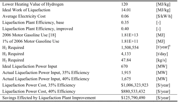
As an example, consider replacing 1% of the 2006 US motor gasoline energy consumption with hydrogen. Assuming that all of the hydrogen required to meet this energy need is liquefied and that industrial electricity costs $0.06 per kilowatt-hour [17], an improvement from 35% to 40% in average hydrogen liquefaction plant efficiency would result in a savings of $125 million per year. As the fraction of hydrogen-powered transportation and the cost of electricity increase, the economic consequences of liquefaction efficiency grow. The details of this hypothetical scenario are summarized in Table 1.

Using hydrogen as an energy carrier implies that its production must experience as little loss as is

Table 1: Economic Savings Due to Improved Hydrogen Liquefaction Efficiency Lower Heating Value of Hydrogen 120 [MJ/kg] Ideal Work of Liquefaction 14.01 [MJ/kg]

Average Electricity Cost 0.06 [$/kW·h]

Liquefaction Plant Efficiency, base 0.35 [-] Liquefaction Plant Efficiency, improved 0.40 [-] 2006 Motor Gasoline Use [18] 1.81E+13 [MJ] 1% of 2006 Motor Gasoline Use 1.81E+11 [MJ]

H2 Required 1,508,554 [t/year]a

H2 Required 4,133 [t/day]

H2 Required 47.84 [kg/s]

Ideal Liquefaction Power Input 670 [MW] Actual Liquefaction Power Input, 35% Efficiency 1,915 [MW] Actual Liquefaction Power Input, 40% Efficiency 1,675 [MW] Liquefaction Power Cost, 35% Efficiency $1,006,323,923 [$/year] Liquefaction Power Cost, 40% Efficiency $880,533,432 [$/year] Savings Effected by Liquefaction Plant Improvement $125,790,490 [$/year]

possible. Liquefaction of hydrogen constitutes a loss: the work of the liquefaction process adds to the total energy invested in each delivered unit of hydrogen. Often the liquefaction work cannot be recovered, but sometimes a portion of the liquefaction energy can be recouped by taking advantage of the properties of the liquid in a subsequent process. Parrish discussed several liquefaction work recovery techniques, including (1) pumping the liquid to high pressure, heating it in a heat exchanger, and extracting work via an expander; (2) using the refrigeration capacity of the liquid in another process, such as an air separation unit; and (3) separating rare gases from the atmosphere by using the low-temperature liquid [19]. These techniques may increase the appeal of storing hydrogen as a liquid in certain applications; however, the energy recovery is limited to 20-60% of the ideal work of liquefaction, which amounts to about 7-20% of the total work in a modern liquefaction plant with 35% Second Law efficiency. Losses in excess of the theoretical minimum work of liquefaction cannot be recovered by any technique. It becomes apparent that the efficiency of the liquefaction cycle directly translates into energy savings in the overall process. The lost liquefaction work detracts from the utility of hydrogen as an energy carrier. Clearly, liquefaction loss must be minimized if hydrogen is to play a meaningful role as an energy storage medium.

1.2. Hydrogen

To improve upon conventional liquefaction systems, an understanding of hydrogen’s unique properties is essential. The differences between hydrogen’s two forms, orthohydrogen and parahydrogen, will be evaluated, as will the transition from ortho to para and the need for effective catalysis of this transition. The effect of parahydrogen concentration on the properties of hydrogen will be discussed, and the significance of the transition with respect to the overall work of liquefaction will be shown.

1.2.1. Orthohydrogen and parahydrogen

Hydrogen is composed of a mixture of orthohydrogen and parahydrogen whose equilibrium composition is a function of temperature. The difference between orthohydrogen and parahydrogen

molecules is the relative orientation of the nuclear spins of the atoms that comprise the hydrogen molecule. The nuclear spins of an orthohydrogen molecule are parallel, while those of a parahydrogen molecule are antiparallel. Ortho and parahydrogen have important property differences.

The equilibrium ortho-para composition of hydrogen is a function of temperature only and can be seen in Figure 2 [20]. The orthohydrogen molecule has three possible quantum substates, while the parahydrogen molecule has only one substate. At high temperatures, all substates become equally populated and the ratio of orthohydrogen to parahydrogen becomes three to one. At room temperature (300 K) the mixture’s equilibrium composition of 75% orthohydrogen and 25% parahydrogen reflects this three to one ratio. Hydrogen with this ortho-para ratio is referred to as normal hydrogen. Conversely, at 20 K the equilibrium mixture is nearly 100% parahydrogen. At an arbitrary temperature the equilibrium mixture is termed equilibrium hydrogen.

Nonequilibrium hydrogen undergoes a slow conversion process in the absence of catalyst [21]. Natural ortho-para conversion occurs when the magnetic dipoles of orthohydrogen molecules in the fluid become close enough to interact [22]. For liquid hydrogen, the rate of orthohydrogen concentration decrease is proportional to the square of the concentration [21]:

2 o o _kx dt dx − = (1)

where xo is the mass fraction of orthohydrogen at time t and k is the rate constant for the reaction. The

value of the rate constant for saturated liquid hydrogen, as measured by Scott et al. [21], is 0.0114 h-1_.

Additionally, this rate changes with density and temperature [22].

In a very slow liquefaction process, hydrogen would be expected to remain at the equilibrium parahydrogen concentration as its temperature is reduced. However, in practice, the characteristic time of the ortho-para conversion is very long compared to the residence time in a liquefaction cycle. If left unaltered, a hydrogen liquefaction system produces liquid hydrogen before the ortho-para conversion has time to occur. The resulting liquid product has a lower-than-equilibrium parahydrogen content.

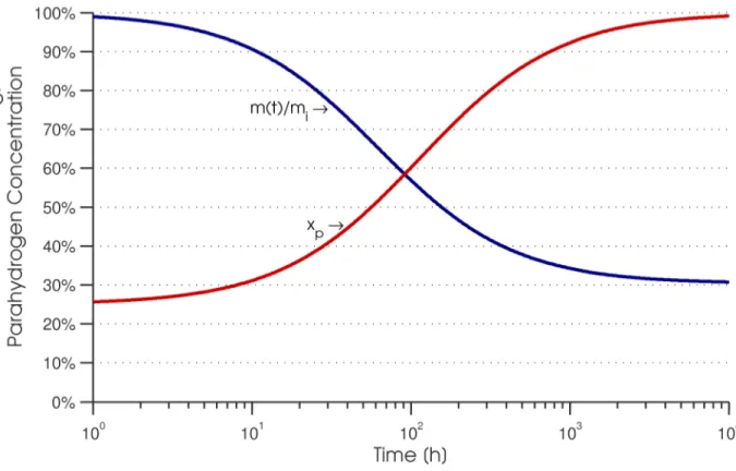
Since parahydrogen is a lower energy state than orthohydrogen, the conversion from ortho to para releases thermal energy. In the previously discussed case where hydrogen is liquefied without any regard to the ortho-para conversion, the liquid product has a para concentration that is below the equilibrium concentration. As time passes, the orthohydrogen in the liquid converts to parahydrogen. Since the conversion is exothermic, some of the liquid product must evaporate to accommodate this heat release. If left unchecked in a completely adiabatic, vented, constant pressure container, the complete self-induced conversion from liquid normal hydrogen to liquid parahydrogen results in evaporation of about 50% of the mixture after 100 hours and 65% after 1000 hours. Integration of equation 1 with a starting orthohydrogen mass fraction of 75% corresponding to normal hydrogen reveals the nature of this boiloff. The liquid mass fraction remaining, which is the liquid mass at time t m(t) divided by the initial mass mi,

behavior presents a problem in a commercial system, where the evaporation of the liquid product is a loss mechanism. Additional refrigeration at the liquid temperature must be supplied to avoid loss of the liquid product; no amount of vessel insulation can prevent this evaporative loss.

Fortunately, the ortho-para conversion can be catalyzed, so that liquefaction plants can remove the conversion energy at higher temperatures. Boiloff and the need for auxiliary refrigeration at liquid temperature are reduced by using catalysts on hydrogen vapor as it cools, thereby producing liquid with high parahydrogen content.

Figure 3: Mass fraction remaining and parahydrogen content for a completely adiabatic, vented, constant pressure container of liquid hydrogen, as a function of time.

1.2.2. Ortho-para catalysts

Indeed, liquefying normal hydrogen and removing all of the conversion heat at the lowest temperature in the cycle is detrimental to a system’s efficiency. In general, the heat of conversion should be removed the highest-possible temperature in the system. This is done by using catalysts that speed up the ortho-para conversion process. Ideally, hydrogen should be kept at equilibrium concentration throughout the cooling process, so that ortho-para conversion is always done at the highest-possible temperature. However, the difficulty of incorporating catalysts into the hydrogen-cooling heat exchangers has led most liquefaction plants to approximate the continuous limit with staged catalyst beds. Four-stage ortho-para conversion is common in industrial-scale plants [23] [24], while other plants have overcome the difficulties associated with continuous ortho-para conversion. Lipman et al. designed and tested a heat exchanger with integrated catalyst material that successfully approached the continuous conversion limit, and alluded to the use of a similar setup in a 26 ton/day Linde hydrogen liquefaction plant in Ontario, California [25]. Sullivan and Zhou also experimented with incorporating a catalyst material into a heat exchanger [26].

A substantial amount of research has been done on ortho-para catalyst materials. The ortho-para transition can be caused by two methods: dissociation and recombination of a hydrogen molecule, and interaction between the magnetic fields of hydrogen nuclei and an external magnetic field [27]. Since dissociative methods lose effectiveness or require energy input at cryogenic temperatures, the magnetic mechanism must be used to catalyze the ortho-para transition in a hydrogen liquefier. Schmauch and Singleton determined that an effective catalyst material “must have a high physical absorptive capacity for hydrogen, a high concentration of ‘active’ or magnetic specie, and a high paramagnetic susceptibility” [27].

Some ortho-para catalyst materials include chromium oxide on alumina [28], hydrous ferric oxide [29][30][31][32][33], Apachi nickel silica gel [27][34], and chromium oxide supported by silica gel [35].

Much research was focused on hydrous ferric oxide, a porous, granular material that is commercially available [36] and for which there is a wealth of experimental data. In particular, Hutchinson [33] studied the kinetics of the catalyzed ortho-para conversion with hydrous ferric oxide and tabulated data detailing the conversion process. This data can be used to estimate the required size of a catalyst bed in a hypothetical liquefaction plant of known capacity.

1.2.3. Property differences between ortho and para

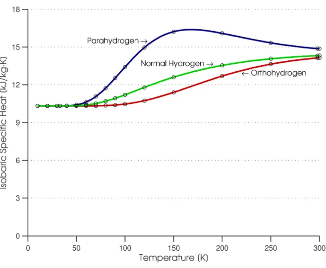
Orthohydrogen and parahydrogen have important and significant property differences. Hust and Stewart summarized the property differences below 300 K [37]. Specific heat and related properties such as enthalpy, entropy and thermal conductivity exhibit the largest differences with changes in the ortho-para composition, while P-v-T data and viscosity are nearly independent of composition. Due to the molecular differences in orthohydrogen and parahydrogen, their rotational modes are excited differently and can be observed in their markedly different specific heats between 70 K and 300 K. The differences in the ideal gas specific heat between orthohydrogen and parahydrogen can be seen in Figure 4.

Haar et al. [38] and Woolley et al. [20] calculated the ideal gas enthalpy, entropy and specific heat of normal, ortho and parahydrogen. For ideal gas mixtures of orthohydrogen and parahydrogen, the properties of the mixture can be determined using mixing equations [37]:

o o p p mix

x

h

x

h

h

=

+

(

)

x

s

x

s

R

x

ln

x

x

ln

x

s

=

+

−

+

where h is specific enthalpy, s is specific entropy, x is the mass fraction of ortho (o) or para (p), and R is the gas constant for hydrogen. The heat of mixing is assumed to be negligible. The third term on the right hand side of equation 3 represents the entropy of mixing. Since properties of orthohydrogen are very rarely reported, it is more convenient to express these equations so that the mixture properties can be calculated from normal and parahydrogen properties. Using equations 2 and 3, the specific enthalpy

Figure 4: Ideal gas isobaric specific heat for parahydrogen, normal hydrogen and orthohydrogen. The circles indicate the original, tabulated data from [20].

and entropy of normal hydrogen (hn and sn) can be written as

o p n

h

4

3

h

4

1

h

=

+

⎟

⎠

⎞

⎜

⎝

⎛

₊

−

+

=

4

3

ln

4

3

4

1

ln

4

1

R

s

4

3

s

4

1

s

Solving equations 4 and 5 for the orthohydrogen enthalpy and entropy and substituting into equations 2 and 3 yields n o p o p mix

x

h

3

4

h

x

3

1

x

h

⎟

+

⎠

⎞

⎜

⎝

⎛

₋

=

(

)

R

x

ln

x

x

ln

x

4

3

ln

4

3

4

1

ln

4

1

R

s

x

3

4

s

x

3

1

x

s

_⎥

−

+

⎦

⎤

⎢

⎣

⎡

⎟

⎠

⎞

⎜

⎝

⎛

₊

+

+

⎟

⎠

⎞

⎜

⎝

⎛

₋

=

[

]

(

)

x

s

0

.

562335

R

R

x

ln

x

x

ln

x

3

4

s

x

3

1

x

s

⎟

+

−

⋅

−

+

⎠

⎞

⎜

⎝

⎛

₋

=

which is consistent with the equation reported by Hust and Stewart [37]. Equations 6 and 8 can be used to determine the enthalpy and entropy of a hydrogen mixture of arbitrary parahydrogen concentration from known normal hydrogen and parahydrogen properties. However, care must be taken to ensure that the normal hydrogen and parahydrogen properties have a consistent reference state, because the mixing equations contain absolute values of enthalpy and entropy that originate from, presumably, different equations of state.

Since the P-v-T properties of normal hydrogen and parahydrogen are virtually identical, the equations above are also useful for higher pressures. Hust and Stewart pointed out that “experimental specific heats confirm the postulate that the specific heat differences due to ortho-para concentration are essentially independent of pressure” [37].

Various equations of state exist for normal and parahydrogen. Leachman conducted a survey of the available experimental data on normal and parahydrogen and formulated “Helmholtz explicit” equations of state to represent the most accurate of these data [39]. These equations, which represent experimental results to within the uncertainty of the data, are currently the most comprehensive and accurate equations of state for hydrogen. Leachman directly compared his parahydrogen equation of state (EOS) to Younglove’s parahydrogen EOS, which is commonly used in engineering. Leachman found that his EOS represented experimental data more accurately and also exhibited fundamentally correct thermodynamic behavior. For example, in Leachman’s EOS the isochoric specific heat of the saturated liquid states increases with temperature, an indication (as Leachman asserts) of thermodynamically correct behavior. This is in direct contrast to the non-monotonic behavior of the corresponding quantities

in the Younglove EOS. The Leachman EOS for both normal and parahydrogen are used in NIST’s thermodynamic property software REFPROP 8.0 [40], and were chosen for the required property lookups in this work.

In this work, to ensure a consistent reference state for the property values obtained from the two different equations of state (normal hydrogen and parahydrogen), the following procedure was used. First, properties were obtained from the EOS at a temperature of 300 K and a pressure of 0.01 bar for both normal hydrogen and parahydrogen. Next, values of enthalpy were obtained from the reduced ideal gas values at 300 K tabulated by Haar et al. [38]. The difference between these enthalpies was noted and compared to the difference in the EOS-calculated enthalpies at 300 K and 0.01 bar. The enthalpy difference between normal and parahydrogen obtained from the EOS was much different than the enthalpy difference calculated from tabulated data. This was because the reference state in the EOS software imposes an arbitrary offset on the absolute values of enthalpy. Most applications only require a difference, so the offset is transparent to the user; however, since enthalpies of two different substances are being compared directly in this work, the reference states must be consistent. Therefore, an offset was added to the normal hydrogen enthalpy that was output from the EOS. After application of the offset, the difference in enthalpy between normal and para was consistent with the expected ideal gas difference. A similar offset was applied to the values of normal hydrogen entropy called from the EOS. By applying these enthalpy and entropy offsets, the normal hydrogen properties called from the EOS become consistently referenced with respect to the parahydrogen properties, allowing proper use of equations 6 and 8 to model the properties of a hydrogen mixture with arbitrary parahydrogen concentration.

1.2.4. Ideal work of liquefaction

Transforming a quantity of hydrogen from a gas at ambient temperature and pressure to a saturated liquid requires work input. This work input is used to extract entropy from the low-temperature hydrogen and reject it at ambient temperature. The amount of work required by a reversible cycle to bring

hydrogen from the starting conditions – in this paper, 300 K, 1 bar and 25% parahydrogen – to the final, saturated liquid state at 1 bar and equilibrium parahydrogen concentration is referred to as the ideal work

of liquefaction.

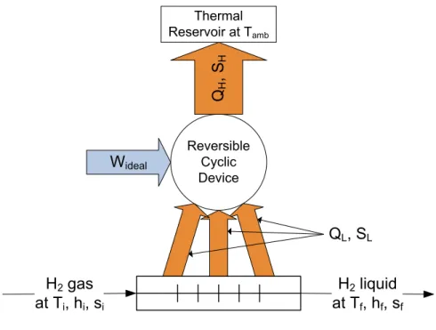
To calculate the ideal work of liquefaction, a stream of hydrogen cooled by a reversible cyclic device is considered, as shown in Figure 5. The quantity of heat removed QL per unit mass m can be

determined by applying the First Law of Thermodynamics to the hydrogen stream:

i f L _{h h} m Q − = − (9)

Next, the heat rejected to the thermal reservoir representing the ambient conditions is determined. The reversible cyclic device has no entropy generation, so that the entropy SL removed from the hydrogen

stream must be equal to the entropy SH rejected to the thermal reservoir. SL is determined by applying the

Second Law to the hydrogen stream. The isothermal heat rejection QH to the ambient temperature Tamb is

determined from the entropy SH.

(

)

(

)

The First Law applied to the cyclic device yields the ideal work per unit mass Wideal/m.

(

)

(

)

The two scenarios shown in Table 2 demonstrate the difference in the ideal work due to ortho-para conversion. For the state of the hydrogen mixture at the initial and final point to be fully defined, three unique thermodynamic parameters must be specified. In addition to temperature and pressure, parahydrogen concentration was specified to accurately define the ideal work. The initial state was

Reversible Cyclic Device

Q

, S

H

gas

at T

, h

, s

H

liquid

at T

, h

, s

W

Q

, S

Figure 5: A stream of hydrogen cooled by a reversible cyclic device. Table 2: Ideal Work of Liquefaction

T [K] P [bar] xp [-] Wideal [kJ/kg]

Initial state 300 1 0.251 -

Final state, saturated liquid, full ortho-para conversion 20 1 0.998 14,327 Final state, saturated liquid, no ortho-para conversion 20 1 0.251 12,147

assumed to have the equilibrium para concentration at 300 K. Two final saturated liquid states at 1 bar are shown: no ortho-para conversion and full conversion to equilibrium.

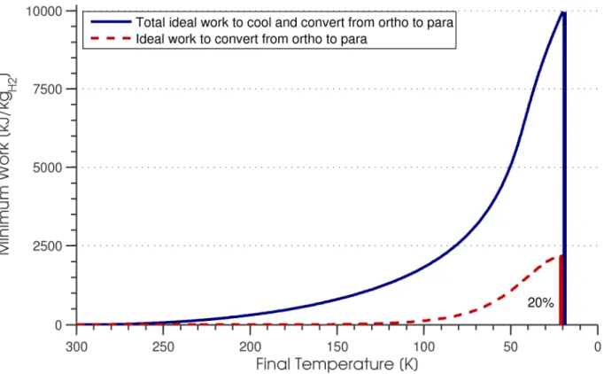
In Table 2 it can be seen that more work is required when the final state consists of equilibrium hydrogen. This result is not surprising given that the conversion from ortho to para is exothermic and results in significant energy release from the product stream. The work associated with the removal of the ortho-para heat of conversion represents a substantial portion of the work required to bring hydrogen to a low temperature. Figure 6 shows the minimum work of cooling and conversion for a stream of gaseous equilibrium hydrogen, and also separately shows only the work of ortho-para conversion. It can be seen

Figure 6: Ideal work vs. temperature for gaseous equilibrium hydrogen. Also shown is the ideal work of ortho-para conversion, which was determined by subtracting the ideal work to cool

gaseous normal hydrogen from the ideal work to cool gaseous equilibrium hydrogen.

that the ortho-para conversion constitutes about 20% of the total work required to cool the hydrogen gas to the saturation temperature. It is also evident that the ideal work associated with ortho-para conversion does not contribute appreciably to the total ideal work until the final temperature is below about 100 K.

1.3. Hydrogen liquefaction plants

This section will begin by introducing some fundamental liquefaction cycles. Additionally, a history of large-scale hydrogen liquefaction and case studies of several commercial plants will be presented. Finally, the particular challenges of hydrogen liquefaction will be reviewed.

1.3.1. Basic hydrogen liquefaction cycles

Although large industrial liquefaction cycles are typically complex, many are based on the Claude cycle [23][24]. In this cycle, hydrogen is both the product and the working fluid. One or more expanders remove work from the working fluid, reducing its temperature. Finally, a Joule-Thomson valve brings the fluid into the two-phase regime, and saturated liquid is removed from the cycle. Makeup gas at the warm end ensures a constant mass in the system. The expander work in the Claude cycle reduces the compressor work and efficiently reduces the temperature of the working fluid. A simple Claude cycle can be seen in Figure 7.

Often, the Claude cycle is modified to have two compressors and is termed a “dual pressure” Claude cycle. The first compresses from low to intermediate pressure, and the second compresses from intermediate to high pressure. The expander operates between the intermediate and low pressures, and its exhaust provides additional cooling to the high-pressure stream. It is also possible to expand between the high and intermediate pressure. The high-pressure stream expands across the J-T valve to the low-pressure storage tank. Low-low-pressure vapor recirculates and cools the intermediate- and high-low-pressure streams. Variations of the dual pressure Claude cycle are widely used in hydrogen liquefaction plants [23], often with a separate product stream that is cooled by the working fluid portion of the cycle. Most plants use liquid nitrogen precooling, multiple stages of ortho-para catalysis, and more than one expander. Figure 8 shows a simple, dual pressure Claude cycle.

Expander Compressor J-T Valve Storage Tank Heat Exchanger Heat Exchanger Heat Exchanger Liquid Product Makeup Gas Compressor Work Expander Work

Figure 7: A simple Claude cycle [41].

1.3.2. Previous and current plants

Industrial hydrogen liquefaction began in the 1950s when the US atomic weapons program and the NASA Apollo missions created demand for large quantities of liquid hydrogen [42][43]. The National Bureau of Standards experimented with large laboratory-scale hydrogen liquefaction starting in 1952 and construction of commercial plants in Ohio, Florida and California occurred in the late 1950s.

Peschka [23] summarized several industrial hydrogen liquefaction plants; this summary can be seen in Table 3 with plants mentioned by Gross et al. [24] and Flynn [44] added. It can be seen that the industry has many years of experience in running plants with tonnage capacities. Additionally, Flynn

Expander Compressor 2 J-T Valve Storage Tank Heat Exchanger Heat Exchanger Heat Exchanger Liquid Product Makeup Gas Expander Work Compressor 1 Compressor Work

Figure 8: A dual pressure Claude cycle [41].

estimated the total US liquid hydrogen capacity to be 172 t/day in 1990, which is an order of magnitude short of the previously estimated 4100 t/day requirement to satisfy 1% of the US motor gasoline consumption. Therefore, many additional industrial-scale liquefaction plants will have to be constructed if hydrogen is to be used as an energy carrier.

In 1961, Vander Arend described one of the aforementioned first generation industrial-scale hydrogen liquefiers: an Air Products 27 ton/day hydrogen production and liquefaction facility [28]. The 17% efficiency of the liquefier does not compare favorably to some of the plants surveyed by Strobridge

Table 3: Hydrogen Liquefaction Plants

Place Producer, Operator Capacity In Operation

Mississippi - Test Facility [23] Air Products 36 t/day 1960 Long Beach, California [23] Air Products 30 t/day 1958 Ontario, California [23] Union Carbide, Linde Division 30 t/day 1962 Sacramento, California [23] [44] Union Carbide, Linde Division 60 t/day 1966a

Los Angeles, California [44] Linde 20 t/day no date given New Orleans, Louisiana [44] Air Products 60 t/day 1976

Niagara Falls, New York [44] Linde 30 t/day no date given Lille, France [23] L’Air Liquide 10 t/day 1985

Rozenburg, Netherlands [23] [24] Air Products 5.0 t/day 1986 Ingolstadt, Germany [24] Linde 4.4 t/day 1992

a _{no longer in operation}

[15]; however, reliability was of paramount importance, which precluded the selection of a thermodynamically superior design. For instance, only one expansion engine is used in the system to avoid potential failures of additional engines, and this expansion engine’s work is not recovered. The cycle consists of a dual pressure hydrogen working fluid with nitrogen precooling and expansion between the intermediate and low hydrogen pressures. A separate product stream of hydrogen is purified and cooled by an auxiliary Freon refrigeration system and finally by the hydrogen working cycle. Ortho-para catalysis using chromic oxide on alumina occurs at “various temperatures,” with no further details given.

Gross et al. described a Linde hydrogen liquefaction plant in Ingolstadt, Germany in 1994 [24]. The plant is based on a Claude cycle and has liquid nitrogen precooling. Two reciprocating compressors provide dual pressure operation, and three turboexpanders in series operate between the high (22 bar) and intermediate (3 bar) pressures. Work is extracted from the expanders, but it is unclear whether or not this work is used to offset the compressor work input. The main J-T valve operates between the high and low (1.3 bar) pressures. Ortho-para catalysis is accomplished in four stages with hydrous ferric oxide catalyst, and acts only on the separate hydrogen product stream. The product stream is thoroughly purified in a pressure swing adsorption plant before entering the liquefier and final purification is achieved at liquid

nitrogen temperature in an additional, low-temperature adsorber. In the publication, a table lists the “thermodynamic efficiency” of the liquefier as 33%. Assuming that the provided compressor powers and flow rates are accurate, a calculation of the Second Law efficiency reveals that this number is accurate only if the energy cost of the liquid nitrogen cooling is neglected. Taking this into account and assuming a nitrogen liquefaction Second Law efficiency of 40%, a 20% overall Second Law efficiency can be calculated for the Ingolstadt plant.

Strobridge conducted a survey of 144 cryogenic refrigerators and liquefiers in 1974 [15]. The second law efficiency, which is sometimes referred to as percent Carnot, defined as

actual ideal W W =

η

was plotted versus the refrigeration capacity for 1.8-9 K, 10-30 K, and 30-90 K machines in Strobridge’s survey, and can be seen in Figure 9. Several large capacity, 10-30 K machines in the survey reported efficiencies between 30 and 40%. In addition to efficiency, Strobridge studied the approximate cost of refrigerators and liquefiers operating in the 1.8-90 K range and established a relationship stating that, as a first approximation, capital cost is proportional to the input power raised to the 0.7 power.

1.3.3. Challenges of hydrogen liquefaction

McIntosh identified hydrogen turboexpanders as one of the most challenging aspects of liquefaction [43]. The low molecular weight and high speed of sound necessitate that very high peripheral speeds be maintained. Material properties restrict the speed and limit each stage to a low pressure ratio. Additional, practical considerations of using turbomachinery with hydrogen include the difficulty of forming reliable seals and the propensity of hydrogen to cause material embrittlement.

Aside from the turbomachinery issues, using hydrogen as the working fluid in a cycle has other problems. In a system with a J-T valve expanding into the saturated regime, only a small portion of the incoming stream is extracted as liquid. Often, the yield is a small portion of the cycle flow rate [41], but

Figure 9: Second Law efficiency versus capacity for cryogenic refrigerators and liquefiers surveyed in 1974 [15].

can be as high as 60% in a dual pressure Claude cycle with ideal components and heat exchangers [23]. The compressor, heat exchangers, and expanders must be sized to handle hydrogen flow rates substantially larger than the plant’s capacity. Extra components, connection points, and hydrogen-filled plumbing introduce more possible leak sites that can be dangerous due to the wide flammability range of hydrogen in air.

The J-T valve is a source of inefficiency. In a J-T valve, the fluid flows from high pressure to low pressure and, provided the fluid has a positive Joule-Thomson coefficient, results in a temperature drop. Fluid flow through a J-T valve generates entropy, which represents a loss in the system and is detrimental to the overall plant efficiency. However, a system with no J-T valve still requires a method of reducing the product stream pressure to the storage pressure. The difficulties of designing an expander to be

operable in the two-phase regime, along with associated reliability concerns, make the J-T valve appealing despite its inherent entropy generation.

The hydrogen makeup gas must be thoroughly purified to avoid the introduction of oxygen and other contaminants into the system. Contaminants other than helium freeze in the system, which can clog a J-T valve or damage an expander. Buildup of frozen oxygen in the product tank can result in an explosion hazard. Purification requirements for hydrogen liquefiers can be as stringent as 1 ppm. McIntosh identifies “explosion proof requirements on equipment and facility design” as an important consideration in liquefier design [43].

The substantial variation in heat load imposed on the cycle by the hydrogen stream presents a challenge in the balancing of the heat exchangers. Recalling Figure 4, the specific heat varies substantially with temperature and parahydrogen concentration. To minimize heat exchange temperature differences, the cycle temperatures and flow rates must be carefully selected. If staged catalyst beds are employed in the cycle, their operating temperatures must also be chosen judiciously.

Baker and Shaner simulated a 250 ton/day, dual pressure Claude cycle with nitrogen precooling and continuous conversion catalysis [45]. Parameters such as feed pressure, recycle return pressure, component efficiencies, heat exchanger temperature differences, and turbine refrigeration levels were varied. The base scenario, whose parameters were selected to provide a realistic simulation, had a Second Law efficiency of 36%. The system losses were itemized and can be seen in Table 4.

Table 4 highlights another challenge: improvements in component efficiency. Baker and Shaner point out that, due to their long development histories, improvements in modern components such as compressors and expanders can be “marginal and difficult to achieve” [45]. However, as plants become larger and more numerous, it may become more economically feasible to develop compressors or expanders specifically suited to a liquefaction cycle’s flow rates and pressure levels. Additionally, heat exchanger losses can be reduced by increases in area. Often, capital costs constrain this area, but the

Table 4: Component Contributions to Cycle Work [45]

Loss [kJ/kg] % of Total Loss

Recycle Compressor 7,343 29.35 Feed Compressor 2,153 8.61 Expanders 3,242 12.96 Heat Exchangers 3,166 12.65 Catalysts 1,021 4.08 Throttling 1,127 4.50 Mixing 408 1.63 Heat Leak 286 1.14 N2 Refrigerator 6,260 25.02 Miscellaneous 15 0.06 Total 25,021 100.00 Ideal Work 14,070

Actual Work 39,091 (36% Carnot)

efficiency improvement associated with lower heat exchange losses would reduce operating costs.

Clearly, hydrogen liquefaction presents many challenges to a cycle designer. Practical challenges arise from hydrogen’s flammability, resistance to being contained by seals, and tendency to cause embrittlement in some common engineering materials. Thorough purification of the feed stream must also be performed to avoid freezing of gaseous impurities and potential explosion hazards due to accumulated oxygen. Hydrogen’s low molecular weight and resultant high speed of sound cause turbine expanders to be less effective. Additionally, hydrogen’s properties present thermodynamic challenges. For example, the ortho-para transition, which must be catalyzed to avoid excessive boiloff losses during storage, contributes a significant amount of the heat removed from the product stream and has a noticeable effect on the cycle work input. Depending on how the catalysts are staged, large heat loads can occur at low temperatures in the system. Finally, the strongly temperature-dependent specific heat and significant property differences between ortho and parahydrogen can cause entropy-generating heat exchanger imbalances in the cycle and demand careful selection of system operating temperatures and flow rates.

CHAPTER 2. CYCLE SIMULATIONS

Based on the assessment of some current liquefaction cycles, several areas of improvement were pursued. Using these ideas and computer simulations of some system configurations, a cycle that addresses the targeted improvements is proposed. The proposed configuration, its features, and its advantages over the typical cycle will be discussed. Additionally, this section will also review the details, assumptions, and inner workings of the simulations used to arrive at and validate the proposed cycle.

2.1. Design goals and component feasibility

Many attributes are desirable in a new cycle design, including overall efficiency, scalability, and simplicity. Obviously, the efficiency of a liquefier determines the energy use and most of the operating cost. Scalability makes a cycle desirable for more diverse applications and allows for less expensive feasibility testing of a large system via the construction of a smaller system. As mentioned by Vander Arend [28], uptime is critical in a commercial liquefaction plant, so simplicity of design was considered throughout the process.

Two plant sizes were considered: a pilot plant, which is a 500 kgH2/day liquefaction plant, and a large plant, which is a 50,000 kgH2/day plant. Since testing of the large plant (a 50 t/day liquefier) would require an enormous capital investment, it is desirable to have the pilot plant very similar in configuration to the large plant so that some validation tests could be applicable to both designs. The desirability of keeping the cycle scalable was considered in the selection of the system components.

Using a high-pressure product stream was considered due to the availability of high pressure from hydrogen sources. In particular, many water electrolyzers operate at high pressure. If a high-pressure electrolyzer were coupled to the liquefier, some compression work could be avoided in the liquefier. The plant would be able to take advantage of the relatively efficient compression process associated with an

electrolyzer rather than having to use a reciprocating machine. In addition, high-pressure hydrogen as the inlet state requires less theoretical ideal work input. Figure 10 shows the reduction in the ideal work associated with a pressurized inlet state. Caution should be used in interpreting Figure 10, however: the reduction in the overall cycle work will not be nearly as dramatic as the reduction in the ideal work. If the cycle is thought of as a refrigerator removing heat from a distributed load, the total amount of heat that must be removed from the hydrogen is virtually identical with the pressurized inlet, since the enthalpy is a very weak function of pressure at room temperature. Thus, for the working portion of the cycle little change occurs, although the heat load imposed by the product stream will be distributed in a different manner because the specific heat changes appreciably with pressure. Effectively, starting with pressurized hydrogen eliminates the work associated with compression of the product stream, which can be small in the context of the entire system. Therefore, with a pressurized inlet, the ideal work may change

Figure 10: Ideal work of liquefaction vs. inlet hydrogen pressure, for a final state of 20 K, 1 bar and 95% parahydrogen

significantly but the overall cycle work may only change slightly. Since the Second Law efficiency is defined as the ratio of the ideal work to the actual work, the Second Law efficiency changes significantly with a change in the inlet state used to determine the ideal work. When examining reported plant efficiencies, it is important to note the reference states with which the ideal work is determined.

In addition to eliminating the product stream compression, a high-pressure inlet state can reduce the severe or infinite peaks in specific heat that occur near or below the critical temperature. The heat capacity of hydrogen is shown in Figure 11 for pressures at and above the critical pressure of 13 bar. It is clear that as the pressure approaches the critical pressure the heat capacity diverges at a temperature of 33 K. At pressures below the critical pressure the heat capacity of all isobars diverge when the fluid undergoes the gas to liquid transition. In many liquefaction cycles the wildly varying heat capacity makes the heat load of the product stream very difficult to match and can lead to unnecessary losses, which suggests that cooling the hydrogen supercritically can lead to improved efficiency.

Simplicity was another important criterion in the cycle design process. Using helium as the working fluid makes some of the hydrogen liquefaction challenges more surmountable. First, helium turboexpanders, which are commonly used in helium liquefaction cycles, operate more effectively than hydrogen turboexpanders. The speed of sound in helium is lower than in hydrogen because of helium’s greater molecular weight. Thus, larger pressure ratios can be achieved in a turbine stage for the same material-limited tip speed. Second, material degradation of components does not occur due to exposure to helium as it can with hydrogen. In addition, helium remains gaseous in the required operating temperatures of the cycle. The combination of a supercritical hydrogen product stream and an all-gaseous helium working fluid eliminates difficulties associated with multiphase expansion. Finally, helium is inert, providing inherent safety in the event of a leak to the environment or to the hydrogen stream.

Figure 11: Specific heat of equilibrium hydrogen vs. temperature at various pressures.

2.2. Proposed cycle

In the simple Claude cycle that typified a conventional hydrogen liquefaction plant, several problems were identified: the inherently inefficient J-T valve, the large hydrogen flow rates in system, and the use of hydrogen turboexpanders.

A system that addresses these problems can be seen in Figure 12. In this configuration, hydrogen passes through a series of heat exchangers until it reaches a temperature slightly above the storage temperature of 20 K, where all of the hydrogen is a liquid rather than a two-phase mixture. The final reduction in temperature to the storage temperature is accomplished with a single-phase wet expander, which will be discussed in more detail in Section 3.2. The heat removed from the hydrogen goes into a refrigeration loop – a helium cycle. The properties of helium are more conducive to the use of

turbomachinery, and helium expanders are commonly used in the cryogenics industry. As mentioned previously, helium is not flammable, so the number of potential hydrogen leak points and the danger of explosion are reduced in comparison with a system using hydrogen as the working fluid.

The design cools a hydrogen stream that is maintained at a supercritical pressure. In this way, the divergent behavior of the hydrogen heat capacity in the two phase region is avoided and is replaced by the relatively benign thermal behavior of the supercritical stream. This allows the temperatures and the capacity flow rates in the helium streams to be better matched to the temperatures and capacity flow rates of the hydrogen stream in the low-temperature heat exchangers, reducing the losses in the cycle.

The elimination of the J-T valve is another advantage of maintaining supercritical hydrogen pressure. Rather than undergoing a distinct phase change like subcritical hydrogen, the supercritical gaseous hydrogen stream gradually increases in density until it reaches liquid density. At the bottom of the system, the hydrogen stream is a high-pressure liquid. A single-phase wet expander extracts a small amount of work from the liquid to reduce its pressure to atmospheric.

Three stages of ortho-para conversion can be seen in Figure 12. Ideally, the ortho-para catalyst would somehow be incorporated into the hydrogen passages in each heat exchanger. However, to keep ease of construction a high priority it was assumed that the first iteration of the system would employ conventional, staged catalysis. The low-pressure helium stream provides cooling to the catalyst bed to maintain the bed at near-isothermal conditions.

The spans of the two lowest-temperature expanders overlap. This configuration provides additional cooling in the critical temperature region where the specific heat of the hydrogen peaks. In addition, there is a substantial heat load due to the ortho-para conversion in the low-temperature catalyst bed. The overlapping expander design also helps to match the thermal load imposed by this catalyst bed.

EXPANDER 1 EXPANDER 2 EXPANDER 3 EXPANDER 4 HYDROGEN COMPRESSOR HELIUM COMPRESSOR SINGLE PHASE WET EXPANDER STORAGE TANK HEAT EXCHANGER 3 HEAT EXCHANGER 4 HEAT EXCHANGER 5 HEAT EXCHANGER 6 HEAT EXCHANGER 7 HEAT EXCHANGER 8 He COOLED CATALYST BED 1 He COOLED CATALYST BED 2 He COOLED CATALYST BED 3 HEAT EXCHANGER 2 HEAT EXCHANGER 1 H2FEED

2.3. Numerical simulations

Both the proposed cycle and several preliminary, simpler cycles were simulated numerically. Initially, a spreadsheet-based model was created that allowed nearly simultaneous solution and graphical output of the solved system operating points. Simple two-, three- and four-stage cycles were solved, but as the systems grew more complex, the deficiencies of the spreadsheet-based solver became apparent and a program-based model was created using MATLAB [46]. The system proposed in the preceding section was fully simulated and the effects of altering basic system parameters were studied.

2.3.1. Spreadsheet-based

A cycle analysis tool was created in a spreadsheet using Microsoft Excel [47]. The motivation behind using spreadsheet-based simulations was the nearly simultaneous graphical outputs that were available when solving a system. In the spreadsheet, a system’s governing energy balance equations were solved while being subjected to constraints imposed by cycle conditions and the Second Law. The variation of parameters to find a maximum in the system efficiency was accomplished using Excel’s Solver add-in program.

Systems explored in the simulations consisted of a hydrogen product stream cooled by a Collins-type helium cycle. Figure 13 shows a diagram of one of the systems that were simulated, and Figure 14 shows the graphical interface associated with this system in the spreadsheet-based solver. The helium is compressed and the high-pressure stream enters the first stage, which consists of heat exchanger (HX) 1, HX 2, and expander 1. The cool, low-pressure helium stream cools the hydrogen and the high-pressure helium stream. The capacity rates of the high-pressure helium and low-pressure helium streams approximately balance each other in heat exchanger 1. Addition of the hydrogen stream causes the downward flow in the heat exchanger to have a larger net capacity flow rate, which results in the tendency of temperatures of the streams to pinch at the top. A fraction of the high-pressure helium is diverted into expander 1 so that heat exchanger 2 has a larger net capacity flow rate in the upward

direction and pinches at the bottom. In a balanced-flow heat exchanger, a low stream-to-stream temperature difference can be maintained, which results in lower entropy generation. Since it is impossible to balance the flows with the addition of the hydrogen stream, the balanced-flow scenario is approximated by allowing the stream temperatures to diverge and converge by altering the relative flow rates of the two helium streams. High-pressure helium diverted into an expander rejoins the low-pressure stream after work is extracted and its temperature is reduced. The unavoidable heat exchanger imbalance losses can be minimized by choosing appropriate flow rates in each expander. Addition of more expanders also helps to reduce this loss.

EXPANDER 1

EXPANDER 2 CATALYST BED

INTEGRATED INTO HEAT EXCHANGER SINGLE-PHASE WET EXPANDER STORAGE TANK HEAT EXCHANGER 4 HEAT EXCHANGER 1 HEAT EXCHANGER 3 HEAT EXCHANGER 2 HYDROGEN COMPRESSOR H2FEED HELIUM COMPRESSOR

Figure 13: A two-stage, helium-cooled hydrogen liquefaction cycle that is typical of the systems simulated.

mdot H2 → → 1.0 compressor ↓ ↑ ← T1 300.0 T2 285.7 Tc 300.0 T2 285.7 top 300.0 T1 P1 1.5 P2 0.3 mdot4 35.7 HX1 35.7 mdot1 Td 177.5 T4 129.7 bottom 153.3 T3 ↓ ↑ ↓ → 16.4 mdot3 expander 1 T3 153.3 Td 177.5 T4 129.7 top 153.3 T3 P3 1.5 mdot4 35.7 HX2 19.2 mdot5 T6 95.2 Te 100.0 T6 95.2 bottom 100.0 T5 P6 0.3 ↓ ↑ ← ← 16 mdot6 Te 100.0 T6 95.2 top 100.0 T5 mdot8 19.2 HX3 19.2 mdot5 Tf 73.9 T8 48.7 bottom 57.8 T7 ↓ ↑ ↓ → 19.2 mdot7 expander 2 T7 57.8 Tf 73.9 T8 48.7 top P7 0.0 mdot8 19.2 HX4 T10 19.0 Tg 20.0 T10 19.0 bottom P10 0.0 ↓ ↑ ← ← 19 mdot10

Figure 14: Graphical output of the spreadsheet-based solver for the two-expander system. The depicted operating point values update when the system is solved.

To completely solve the system, some assumptions were necessary. A set of temperatures was assumed for the hydrogen stream. The hydrogen stream temperatures, after the system was solved, were changed until a maximum efficiency was approached. It was assumed for simplicity that the temperature of the high-pressure helium stream would be the same as the temperature of the hydrogen stream at each stage point.

Following the work of Minta and Smith [48] for a given liquefier design, the total heat exchanger area is most effectively distributed when the value of ∆T/T, defined as

T

T

T

T

T

−

₌

∆

is given a constant value at all stage points. The ∆T/T constraint was not strictly enforced at each stage point, but a constraint was imposed to prevent the stream-to-stream temperature difference from becoming less than this value. When the system efficiency was maximized, the actual ∆T/T values tended to push this constraint to its limit at each stage point as expected. This constraint limits the total heat exchange area in the simulation – without it, the stream-to-stream temperature differences would be driven to zero, making the efficiency greater but implying infinite heat exchange area.

In the catalyst beds it was assumed that the low-pressure helium cooling stream maintained the temperature of the hydrogen stream at a constant value. The change in enthalpy of the hydrogen in a catalyst bed occurred solely because of the change in the parahydrogen concentration. The heat given off by the ortho-para conversion was taken up by the low-pressure helium stream. This isothermal catalyst bed behavior has been approximated in experiments. For example, Hutchinson maintained small catalyst beds at nearly constant temperature to determine ortho-para conversion rates for hydrous ferric oxide catalyst material [33]. In the simulations in this work, it was also assumed that the catalyst beds were large enough to allow the hydrogen to reach the equilibrium parahydrogen concentration.

Initial simulations were performed to determine the value of additional stages. In these simulations, the adiabatic efficiencies of each expander and the isothermal efficiencies of each compressor were assumed to be 80% and 65%, respectively. The ∆T/T value at each stage was restricted to 5%. The temperature of the thermal reservoir into which the compressors reject heat was assumed to be the ambient temperature of 300 K. The Second Law efficiency was defined as

(

)

(

)

[

]

N 1 i ) i exp( 2 H , comp He , comp ideal , on liquefacti system , net system

s

s

T

h

h

W

W

W

W

W

−

−

−

−

+

=

=

∑

η

Table 5: Efficiencies for Two-, Three- and Four-Stage Cycles Number of Stages Second Law Efficiency

2 0.163 3 0.33 4 0.356

where the final state is hydrogen at 20 K, 1 bar and 95% parahydrogen and the initial state is at 300 K, 1 bar and 25% parahydrogen. The 95% parahydrogen concentration of the final state is a typical target value for liquefaction plants [24]. Table 5 shows the overall efficiencies of two-, three- and four-stage cycles. As can be seen in Table 5, increasing the number of stages from two to three results in a large efficiency increase of 0.167, while increasing from three to four yields a less pronounced gain of only 0.026. Numerical problems surfaced with cycles having greater than four stages, and these systems were not solved. From the trend shown in Table 5, it is expected that adding another stage in a cycle would not be worth the considerable associated increase in capital cost.

While the spreadsheet-based simulations are capable of solving the system, much care had to be taken in doing so. With improper choices for the initial values of the expander mass flows, the system encountered difficulty in finding the solution. Solving the system often became laborious because the solver’s sensitivity to the initial guess values required manual adjustment of parameters until the system was capable of convergence. Despite the convenience of the quickly updating graphical interface, the deficiencies of the spreadsheet-based solver showed that a more robust solving program was needed.

2.3.2. Program-based

In order to take advantage of powerful built-in optimization algorithms, freedom to compartmentalize portions of code into subfunctions, and ease of interfacing with REFPROP for fluid properties, MATLAB programs (m-files) were created to simulate the system. The heart of the program-based simulations consists of two files: the cycle solver (cycle.m) and the cycle optimizer (optimize.m). For an input of the system flow rates, the cycle solver can return either (1) a value related to the cycle