Analytical cache models with applications to cache partitioning in time-shared systems

Analytical Cache Models with Applications to

Cache Partitioning in Time-Shared Systems

by

Gookwon Edward Suh

Submitted to the Department of Electrical Engineering and Computer Science in partial fulfillment of the requirements for the degree of

Master of Science

at the

MASSACHUSETTS INSTITUTE OF TECHNOLOGY

KER

February 2001 MASSACHUSETTS _INSTITUTE

OF TECHNOLOGY

@Massachusetts Institute of Technology.

All rights reserved. _APR

₀₀₀₁

LIBRARIES Author...

Department of Electrical Engineering and Computer Science February 5, 2001

Certified by... ...

Srinivas Devadas Professor of Computer Science Thesis Supervisor

Certified by... ... ... ...

Larry Rudolph Principal Research Scientist Thesis Supervisor

A ccepted by ... .. ...

Arthur C. Smith Chairman, Committee on Graduate Students Department of Electrical Engineering and Computer Science

Analytical Cache Models with Applications to Cache

Partitioning in Time-Shared Systems

by

Gookwon Edward Suh

Submitted to the Department of Electrical Engineering and Computer Science on February 5, 2001, in partial fulfillment of the

requirements for the degree of Master of Science

Abstract

This thesis proposes an analytical cache model for time-shared systems, which esti-mates the overall cache miss-rate from the isolated miss-rate curve of each process when multiple processes share a cache. Unlike previous models, our model works for any cache size and any time quantum. Trace-driven simulations demonstrate that the estimated miss-rate is very accurate for fully-associative caches. Since the model provides a fast and accurate way to estimate the effect of context switching, it is use-ful for both understanding the effect of context switching on caches and optimizing cache performance for time-shared systems.

The model is applied to the cache partitioning problem. First, the problems of the LRU replacement policy is studied based on the model. The study shows that proper cache partitioning can enable substantial performance improvements for short or mid-range time quanta. Second, the model-based partitioning mechanism is implemented and evaluated through simulations. In our example, the model-based partitioning improves the cache miss-rate up to 20% over the normal LRU replacement policy.

Thesis Supervisor: Srinivas Devadas Title: Professor of Computer Science

Thesis Supervisor: Larry Rudolph Title: Principal Research Scientist

Acknowledgments

It has been my pleasure to work under the expert mentorship of Doctor Larry Rudolph and Professor Srinivas Devadas. Larry worked with me on daily basis, discussing and advising every aspect of my research work. His encouragement and advice were essential to finishing this thesis. Srini challenged me to organize my ideas and focus on real problems. His guidance was a tremendous help in finishing this thesis. I would like to thank both my advisors for their support and advice throughout my master's work.

The work described in this thesis would not have been possible without the help of my fellow graduate students in Computational Structures Group. Dan Rosenband has been a great officemate, helping me to get used to the life at LCS, both profes-sionally and personally. Derek Chiou was always generous with his deep technical knowledge, and helped me to choose the thesis topic. My research started from his Ph.D. work. Enoch Peserico provided very helpful comments on my cache models with his knowledge in algorithms and theory. Peter Portante taught me about real operating systems.

Beyond my colleagues in CSG, I was fortunate to have great friends such as Todd Mills and Ali Tariq on the same floor. We shared junky lunches, worked late nights and hung out together. Todd also had a tough time reading through all my thesis drafts and fixing my broken English writing. He provided very detailed comments and suggestions. I would like to thank them for their friendship and support.

My family always supported me during these years. Their prayer, encourage-ment and love for me is undoubtedly the greatest source of my ambition, inspiration, dedication and motivation. They have given me far more than words can express.

Most of all, I would like to thank God for His constant guidance and grace through-out my life. His words always encourage me:

See, I am doing a new thing! Now it springs up; do you not perceive it? I am making a way in the desert and streams in the wasteland (Isaiah 43:19).

Contents

1 Introduction

1.1 M otivation . . . . 1.2 Previous Work . . . . 1.3 The Contribution of This Research . . 1.4 Organization of This Thesis . . . . 2 Analytical Cache Model

2.1 Overview . . . . 2.2 Assumptions . . . . 2.3 Fully-Associative Cache Model . . . . . 2.3.1 Transient Cache Behavior . . . 2.3.2 The Amount of Data in a Cache 2.3.3 The Amount of Data in a Cache 2.3.4 Overall Miss-rate . . . . 2.4 Experiments . . . . 2.4.1 Cache Flushing Cases . . . . 2.4.2 General Cases . . . .

. . . . . . . . . . . . . . . . Starting with an Empty for the General Case . . . . . . . . . . . . . . . . . .

3 Cache Partitioning Based on the Model 3.1 Specifying a Partition . . . . 3.2 Optimal Partitioning Based on the Model

3.2.1 Estimation of Optimal Partitioning 3.3 Tradeoffs in Cache Partitioning . . . . 4 Cache Partitioning Using LRU Replacement

4.1 Cache Partitioning by the LRU Policy

4.2 Comparison between Normal LRU and LRU with Optimal Partitioning 4.2.1 The Problem of Allocation Size . . . . 4.2.2 The Problem of Cache Layout . . . . 4.2.3 Sum m ary . . . . 4.3 Problems of the LRU Replacement Policy for Each Level of Memory

H ierarchy . . . . 4.4 Effect of Low Associativity . . . . 4.5 More Benefits of Cache Partitioning . . . . Cache 9 11 13 14 15 16 16 16 17 18 20 22 25 27 27 29 32 33 34 36 36 44 . . . . 4 4 45 45 48 49 52 53 54 . . . . . . . . . . . . . . . .

5 Partitioning Experiments 56

5.1 Implementation of Model-Based Partitioning . . . . 56

5.1.1 Recording Memory Reference Patterns . . . . 57

5.1.2 _{Cache Partitioning . . . .} 58

5.2 Cache Partitioning Based on Look-Ahead Information . . . . 61

5.3 Experimental Results . . . . 62

6 Conclusion 68

Chapter 1

Introduction

The cache is an important component of modern memory systems, and its perfor-mance is often a crucial factor in determining the overall perforperfor-mance of the system. Processor cycle times have been reduced dramatically, but cycle times for memory access remain high. As a result, the penalty for accessing main memory has been increasing, and the memory access latency has become the bottleneck of modern pro-cessor performance. The cache is a small and fast memory that keeps frequently

accessed data near the processor, and can therefore reduce the number of main mem-ory accesses [13].

Caches are managed by bringing in a new data block on demand, and evicting a block based on a replacement policy. The most common replacement policy is the least recently used (LRU) policy, which evicts the block that has not been accessed for the longest time. The LRU replacement policy is very simple and at the same time tends to be efficient for most practical workloads especially if only one process is using the cache.

When multiple running processes share a cache, they experience additional cache misses due to conflicts among processes. In the past, the effect of context switches was negligible because both caches and workloads were small. For small caches and workloads, reloading useful data into the cache only takes a small amount of time. As a result, the number of misses caused by context switches was relatively small compared to the total number of misses over a usual time quantum.

However, things have changed and the context switches can severely degrade cache performance in modern microprocessors. First, caches are much larger than before. Level 1 (LI) caches range up to a few MB [10], and L2 caches are up to several MB [6, 21]. Second, workloads have also become larger. Multimedia processes such as video or audio clips often consume hundreds of MB. Even many SPEC CPU2000 benchmarks now have a memory footprint larger than 100 MB [14]. Finally, context switches tend to cause more cache pollution than before due to the increased number of processes and the presence of streaming processes. As a result, it can be cru-cial for modern microprocessors to minimize inter-process conflicts by proper cache partitioning [29, 17] or scheduling [25, 30].

A method of evaluating cache performance is essential both to predict miss-rate and to optimize cache performance. Traditionally, simulations have, virtually ex-clusively, used for cache performance evaluation [32, 24, 20]. Although simulations provide accurate results, simulation time is often too long. Moreover, simulations do not provide any intuitive understanding of the problem to improve cache perfor-mance. To predict cache miss-rate faster, hardware monitoring can also be used [33]. However, hardware monitoring is limited to the particular cache configuration that is implemented. As a result, both simulations and hardware monitoring can only be used to evaluate the effect of context switches [22, 18].

To provide both performance prediction and the intuition to improve it, analytical cache models have been developed. One such approach is to analyze a particular form of source codes such as nested loops [12]. Although this method is both accurate and intuitive, it is limited to particular types of algorithms. The other way to analytically model caches is extracting parameters of processes and combining them with other parameters defining the cache [1, 28]. These methods can predict the general trend of cache behavior. For the problem of context switching, however, they only focus on very long time quantum. Moreover, their input parameters are difficult to extract and almost impossible to obtain on-line.

This paper presents an analytical cache model for context switches, which can estimate overall miss-rate accurately for any cache size and any time quantum. The

characteristics for each process is given by the miss-rate as a function of cache size when the process is isolated, which can be easily obtained either on-line or off-line. The time quanta for each process and cache size are also given as inputs to the model. With this information, the model estimates the overall miss-rate of a given cache size running an arbitrary combination of processes. The model provides good estimates for any cache size and any time quantum, and is easily applied to real problems since the input miss-rate curves are both intuitive and easy to obtain in practice. Therefore, we believe that the model is useful for any study related to the effect of context switches on cache memory.

The problem of cache partitioning among time-shared processes serves as the ex-ample of the model's applications. Optimal cache partitioning is studied based on the model, which shows the way to determine the best cache partition and the prob-lems with the LRU replacement policy. From the study, a model-based partitioning mechanism is implemented. The mechanism obtains the miss-rate characteristic of each process by off-line profiling, and performs on-line cache allocation according to the combination of processes that are executing at any given time.

1.1

Motivation

Figure 1-1 (a) shows the trace-driven simulation results when six processes are sharing the same cache. In the figure, the x-axis represents the number of memory references per time quantum, and the y-axis represents the cache miss-rate expressed as a per-centage. The number of memory references per time quantum is assumed to be the same for all processes. The Li caches are 256-KB 8-way associative, separate for instruction stream and data stream. The L2 cache is a 2-MB 16-way associative unified cache. Two copies of three benchmarks are simulated, which are the image understanding program from the data intensive systems benchmark suite [23], vpr and twolf from the SPEC CPU2000 benchmark suite [14].

In the figure, the miss-rate of the Li instruction cache is very close to 0% and the miss-rate of the Li data cache is around 5%. However, the L2 cache miss-rate shows

-+- Li Inst -- Li Data -*- L2 90 80 70 60 50 40 30 20 10 0-1 90 80 70( 60 ' 5 0 40 30* 20 10-0 -+- LRU -0- Ideal 6 7 106 10 Time Quantum (b) 108

of time quanta, 256 KB 8-way Comparison of cache miss-rate

10

Time Quantum (a)

Figure 1-1: (a) Cache miss-rate for different length Li, 2 MB 16-way L2 (LI Inst is almost 0%). (b)

with/without partitioning. a) C', C', 10 10 108 --+ 05

that the impact of context switches can be very severe even for realistic time quanta. For the time quantum of a million memory references, the L2 cache miss-rate is about 80%, but for longer time quanta the miss-rate is almost 0%. This means that the benchmarks would get miss-rates close 0% if they use the cache alone, and therefore context switches cause most of L2 cache misses. Even for the longer time quanta, the inter-process conflict misses are a significant fraction of the total L2 misses. Therefore, this example shows that context switches can severely degrade the cache performance even for systems with a very high clock speed.

Figure 1-1 (b) shows the comparison of L2 miss-rates with and without cache partitioning for the same cache configuration and the same benchmark set as before. The normal LRU replacement policy is used for the case without cache partitioning. For the cache partitioning case, the information of next reference time is recorded from the trace, and a new block replaces other process' block only if the new block is accessed again before other process' block. The result shows that for a certain range of time quanta, such as one million memory references, partitioning can significantly reduce the miss-rate.

1.2

Previous Work

Several early investigations of the effects of context switches use analytical models. Thiebaut and Stone [28] modeled the amount of additional misses caused by context switches for set-associative caches. Agarwal, Horowitz and Hennessy [1] also included the effect of conflicts between processes in their analytical cache model and show that inter-process conflicts are noticeable for a mid-range of cache sizes that are large enough to have a considerable number of conflicts but not large enough to hold all the working sets. However, these models work only for long enough time quanta, and require information that is hard to collect on-line.

Mogul and Borg [22] studied the effect of context switches through trace-driven simulations. Using a timesharing system simulator, their research shows that system calls, page faults, and a scheduler are the main source of context switches. They

also evaluate the effect of context switches on cycles per instruction (CPI) as well as the cache miss-rate. Depending on cache parameters the cost of a context switch appears to be in the thousands of cycles, or tens to hundreds of microseconds in their simulations.

Stone, Turek and Wolf [26] investigated the optimal allocation of cache memory among two or more competing processes that minimizes the overall miss-rate of a cache. Their study focuses on the partitioning of instruction and data streams, which can be thought as multitasking with a very short time quantum. Their model for this case shows that the optimal allocation occurs at a point where the miss-rate deriva-tives of the competing processes are equal. The LRU replacement policy appears to produce cache allocations very close to optimal for their examples. They also describe a new replacement policy for longer time quanta that only increases cache allocation based on time remaining in the current time quantum and the marginal reduction in miss-rate due to an increase in cache allocation. However, their policy simply as-sumes the probability for a evicted block to be accessed in the next time quantum as a constant, which is neither validated nor is it described how this probability is obtained.

Thiebaut, Stone and Wolf applied their partitioning work [26] to improve disk cache hit-ratios [29]. The model for tightly interleaved streams is extended to be applicable for more than two processes. They also describe the problems in applying the model in practice, such as approximating the miss-rate derivative, non-monotonic miss-rate derivatives, and updating the partition. Trace-driven simulations for 32-MB disk caches show that the partitioning improves the relative hit-ratios in the range of 1% to 2% over the LRU policy.

1.3

The Contribution of This Research

Our analytical model differs from previous efforts in that previous work has tended to focus on some specific cases of context switches. The new model works for any time quanta, whereas the previous models focus only on long time quanta. Therefore, the

model can be used to study multi-tasking related problems on any level of caches. Since a lower level cache only sees memory references that are missed in the higher level, the effective time quantum decreases as we go up the memory hierarchy. More-over, the model is based on a miss-rate curve that is much easier to obtain compared to footprints or the number of unique cache blocks that previous models require, which makes the model very helpful for developing solutions for cache optimization problems.

Our partitioning work based on the analytical cache model also has advantages over previous work. First, our partitioning works for any level of memory hierarchy for any range of time quantum, unlike, for instance, Thiebaut, Stone and Wolf's partitioning algorithm which can only be applied to disk caches. Further, the model provides a more complete understanding of optimal partitioning for different cache sizes, and time quanta.

1.4

Organization of This Thesis

The rest of this thesis is organized as follows. In Chapter 2, we derive an analytical cache model for time-shared systems. Chapter 3 discusses cache partitioning based on the model. This optimal partitioning is compared to the standard LRU replacement policy and the problems of the LRU replacement policy are discussed in Chapter 4. In Chapter 5, we implement a model-based cache partitioning algorithm and evaluate the implementation by simulations. Finally, Chapter 6 concludes the paper.

Chapter 2

Analytical Cache Model

2.1

Overview

The analytical cache model estimates the cache miss-rate for a multi-process situation when the cache size, the length of each time quantum, and a miss-rate curve for each process as a function of the cache size are known. The cache size is given by the number of cache blocks, and the time quantum is given by the number of memory references. Both are assumed to be constants (See Figure 2-1 (a)).

2.2

Assumptions

The derivation of the model is based on several assumptions. First, the memory reference pattern of each process is assumed to be represented by a miss-rate curve that is a function of the cache size, and this miss-rate curve does not change over time. Although, real applications do have dynamically changing memory reference patterns, the model's results show that the average miss-rate works very well. For abrupt changes in the reference pattern, multiple miss-rate curves can be used to estimate an overall miss-rate.

Second, we assume that there is no shared address space among processes. Other-wise, it is very difficult to estimate the amount of cache pollution since a process can use data brought into the cache by other processes. Although processes may share

miss-rate curves (mi(x))

time quanta (Ti) Cache Model - overall miss-rate

cache size (C)

(a)

Process 1 Process 2

T1 T2o

Process N Process 1 Process 2

... TN T1 T2

(b)

* Time

Figure 2-1: (a) The overview of an analytical cache model. (b) Round-robin schedule.

a small amount of shared library code, this assumption is true for common cases where each process has its own virtual address space and the shared memory space is negligible compared to the entire memory space that is used by a process.

Finally, we assume that processes are scheduled in a round-robin fashion with a fixed time quantum for each process as shown in Figure 2-1 (b). Also, we assume the least recently used (LRU) replacement policy is used. Note that although the round-robin scheduling and the LRU policy are assumed for the model, models for other scheduling methods and replacement policies can be easily derived in a similar manner.

2.3

Fully-Associative Cache Model

This section derives a model for fully-associative caches. Although most real caches are set-associative caches, a model for fully-associative caches is very useful for under-standing the effect of context switches because the model is simple. Moreover, since a set-associative cache is a group of fully-associative caches, a set-associative cache model can be derived based on the fully-associative model [27].

2.3.1

Transient Cache Behavior

Once a cache gets filled with valid data, a process can be considered to be in a steady state and by our assumption, the miss-rate for the process does not change. The initial burst of cache misses before steady state is reached will be referred to as the

miss-rate transient behavior.

For special situations, where a cache is dedicated to a single process for its entire execution, the transient misses are not important because the number of misses in the transient state is negligible compared to the number of misses over the entire execution, for any reasonably long execution.

For multi-process cases, a process experiences transient misses whenever it restarts from a context switch. Therefore, the effect of transient misses could be substantial causing performance degradation. Since we already know the steady state behavior from the given miss-rate curves, we can estimate the effect of context switching once we know the transient behavior.

We make use of the following notations:

t the number of memory references from the beginning of a time quantum.

x(t) the number of cache blocks belong to a process after t memory references.

m(x) the miss-rate for a process with cache size x.

Note that our time t starts at the beginning of a time quantum, not the beginning of execution. Since all time quanta for a process are identical by our assumption, we consider only one time quantum for each process.

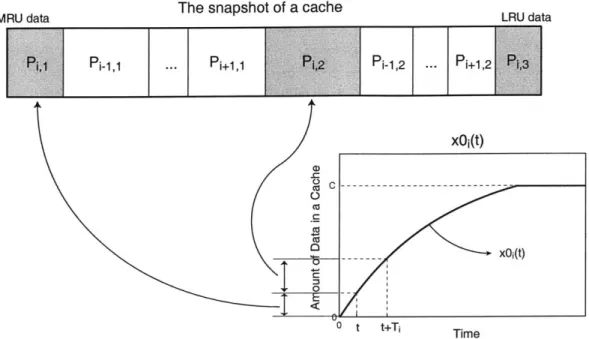
Figure 2-2 (a) shows a snapshot of a cache at time to, where time t is the number of memory references from the beginning of the current time quantum. Although the cache size is C, only part of the cache is filled with the current process' data at that time. Therefore, the effective cache size at time to can be thought of as the amount of current process' data x(to). The probability of a cache miss in the next memory

m(x) for the current process mriss(to) Cache size x(to) The currentI process' data

Other process' data/Empty

The cache at time to (a)

0

~0

-0 2~

Miss probability: Pmiss(t)

Te number of misses \\ Integ rate Time The length of a time quantum (T) (b)

Figure 2-2: (a) The probability to miss at time to. (b) The number of miss-rate from

Pmiss (t) curve.

reference is given by

Pmiss(to) = m(x(to)) (2.1)

where m(x) is a steady state miss-rate for the current process when the cache size is

a:.

Once we have Pmiss (to), it is easy to estimate the miss-rate over the time quantum. Since one memory reference can cause one miss, the number of misses for the process over a time quantum can be expressed as a simple integral as shown in Figure 2-2 (b):

misses = Pmiss(t)dt = m(x(t))dt

0 f

(2.2)

where T is the number of memory references in a time quantum. The miss-rate of the process is simply the number of misses divided by the number of memory references:

miss-rate = 1 PTs(t dt = m(x(t))dt (2.3)

-3

2.3.2

The Amount of Data in a Cache Starting with an Empty

Cache

Now we need to estimate x(t), the amount of data in a cache as a function of time. We shall use of the case where a process starts executing with an empty cache to estimate cache performance for cases when a cache get flushed for every context switch. Virtual address caches without process ID are good examples of such a case. We will show how to estimating x(t) for the general case as well.

Consider x' (t) as the amount of the current process' data at time t for an infinite size cache. We assume that the process starts with an empty cache at time 0. There are two possibilities for x (t) at time t + 1. If the (t + 1)h memory reference results in a cache miss, a new cache block is brought into the cache. As a result, the amount of the process's cache data increases by one. Otherwise, the amount of data remains the same. Therefore, the amount of the process' data in the cache at time t + 1 is given by

X0 (t + 1) = X (t) + 1 when the (t + 1)th reference misses (2.4)

X CO(t) otherwise.

Since the probability for the (t

+

E[x'(t + 1)] = _{E[x (t) - (1 - m(x (t))) + (x (t) + 1) -m(x (t))]}

= E[x (t) + 1 -m(x (t))] (2.5)

= E[x (t)] + E[m(x (t))].

Assuming that m(x) is convex', we can use Jensen's inequality

[8]

'If a replacement policy is smart enough, marginal gain of having one more cache block

equation as a function of E[x (t)].

E[x (t + 1)] > E[x (t)] + m(E[x (t)]). (2.6)

Usually, a miss-rate changes slowly. As a result, for a short interval such as from x to x + 1, m(x) can be approximated as a straight line. Since the equality in Jensen's inequality holds if the function is a straight line, we can approximate the amount of data at time t

+

E[xO (t + 1)] E[x (t)] + m(E[x (t)]). (2.7)

We can calculate the expectation of xO (t) more accurately by calculating the probability for every possible value at time t (See Appendix A). However, calculating a set of probabilities is computationally expensive. Also, our experiments show that the approximation closely matches simulation results.

If we approximate the amount of data x (t) to be the expected value E[x (t)], xc (t) can be expressed with a differential equation:

x (t + 1) - x, (t) = m(x (t)), (2.8)

which can be easily calculated in a recursive manner.

For the continuous variable t, we can rewrite the discrete form of the differential equation 2.8 to a continuous form:

dx~

=x mn(X ). _(2.9)

dt

Solving the differential equation by separating variables, the differential equation becomes

t = fxo(t) dx'. (2.10)

]O)

m(x), and then x (t) can be written as a function of t:

X0(t) = M 1(t + M(x (0))) (2.11)

where M-1 (x) represents the inverse function of M(x).

Finally, for a finite size cache, the amount of data in the cache is limited by the size of the cache C. Therefore, x4_{(t), the amount of a process' data starting from an}

empty cache, is written by

xO(t) = MIN[x (t), C] = MIN[M-1 (t + M(O)), C]. (2.12)

2.3.3

The Amount of Data in a Cache for the General Case

In Section 2.3.1, it is shown that the miss-rate of a process can be estimated if the amount of the process' data as a function of time x(t) is given. In the previous section, x(t) is estimated when a process starts with an empty cache. In this section, the amount of a process' data at time t is estimated for the general case when a cache is not flushed at a context switch. Since we now deal with multiple processes, a subscript i is used to represent Process i. For example, xi(t) represents the amount of Process i's data at time t.

The estimation of xi(t) is based on round-robin scheduling (See Figure 2-1 (b)) and the LRU replacement policy. Process i runs for a fixed length time quantum Ti. During each time quantum, the running process is allowed to use the entire cache. For simplicity, processes are assumed to be of infinite length so that there is no change in the scheduling. Also, the initial startup transient from an empty cache is ignored since it is negligible compared to the steady state.

To estimate the amount of a process' data at a given time, imagine the snapshot of an infinite size cache after executing Process i for time t as shown in Figure 2-3. We assume that time is 0 at the beginning of the process' time quantum. In the figure, the blocks on the left side show recently used data, and blocks on the right side shows old data. P,k represents the data of Process

j,

MRU data The snapshot of a cache i-1,1 ... Pi+1,1 2[ C)E 10 E-i < i 0 t t+Ti LRU data i-1,2 ... - Pi+1,2 x0i(t) Time

Figure 2-3: The snapshot of a cache after running Process i for time t.

the most recent time quantum when the data are referenced. From the figure, we can obtain xi(t) once we know the size of all P,k blocks.

The size of each block can be estimated using the xf(t) curve from Equation 2.12, which is the amount of Process i's data when the process starts with an empty cache. Since x(t) can also be thought of as the expected amount of data that are referenced from time 0 to time t, x(T) is the expected amount of data that are referenced over one time quantum. Similarly, we can estimate the amount of data that are referenced over k recent time quanta to be xO(k -T). As a result, the expected size of Block P,k can be written as P, k x(t + (k - 1) -T) - x4(t + (k -2) -T) x (k - T) - x" ((k - 1) -T) if j is executing otherwise

where we assume that x (t) = 0 if t < 0.

xi(t) is the sum of Pi,k blocks that are inside the cache of size C in Figure 2-3. If

we define li(t) as the maximum integer value that satisfies the following inequality, (2.13)

0 C 0 as C xi(O)

0 tstart(i,2) tend(i,2) Time

Figure 2-4: The relation between xi(t) and xi(t).

Q2(t) + 1 represents how many Pi,k blocks are in the cache.

1i(t) N N

- xt± (l(t) -1) -Ti) + ? (li(t) - T) < C

k=O j=1 _j=1,jAi

(2.14)

where N is the number of processes. From li(t) and Figure 2-3, the expectation value of xi(t) is

N

{xfI(t +l (t).-T) if x i(t+li(t) + + H x (lI(t) -Tj) < C

xi~t N jlj

C - xo(li(t) -Tj) otherwise.

j=1,joi

(2.15)

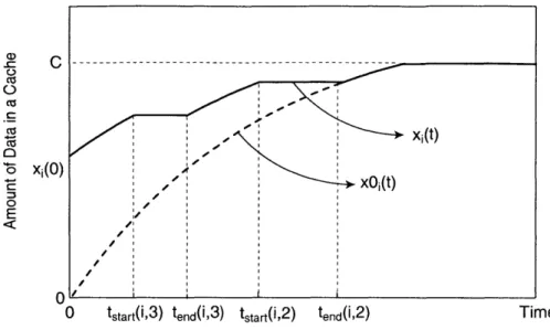
Figure 2-4 illustrates the relation between x (t) and x₂(t). In the figure li(t) is assumed to be 2. Unlike the cache flushing case, a process can start with some of its data left in the cache. The amount of initial data xi(O) is given by Equation 2.15. If the least recently used (LRU) data in a cache does not belong to Process i, xi(t) increases the same as xo(t). However, if the LRU data belongs to Process i, xi(t)

xij~t)

xOi(t)

does not increase on cache misses since Process i's block gets replaced.

Define tstart(j, k) as the time when the kth MRU block of Process

j

from the cache (See Figure 2-3). tstart(j, k) and tend(j, k) specify the flat segments in

Figure 2-4 and can be estimated from the following equations based on Equation 2.13.

N X" (tstart (j, k) + (k - 1) Tj) + x ((k - 1) -Tp) C. (2.16) p=1,pf j N x$(tend(j, k) + (k - 2) Tj)+ x3 x((k -1) Tp) C. (2.17) p=1,pf j

tstart(j, 1j(t) + 1) would be zero if the above equation results in a negative value for

given

j

2.3.4

Overall Miss-rate

Section 2.3.1 explains how to estimate the miss-rate of each process when the amount of the process' data as a function of time xi(t) is given. The previous sections showed how to estimate xi(t). This section presents the overall miss-rate calculation.

When a cache uses virtual address tags and gets flushed for every context switch, each process starts a time quantum with an empty cache. In this case, the miss-rate of a process can be estimated from the results of Section 2.3.1 and 2.3.2. From Equation 2.3 and 2.12, the miss-rate for Process i can be written by

1 fT

miss-ratei =-

J

Ti

If a cache uses physical address tags or has process ID's with virtual address tags, it does not have to be flushed at a context switch. In this case, the amount of data

xi(t) is estimated in Section 2.3.3. The miss-rate for Process i can be written by

I Ti

miss-ratei = - mi (xi (t)) dt _(2.19)

Ti fo

where xi(t) is given by Equation 2.15.

For actual calculation of the miss-rate, tstart(j, k) and tend(j, k) from Equation 2.16 and 2.17 can be used. Since tstart(j, k) and ted(j, k) specify the flat segments in

Figure 2-4, the miss-rate of Process i can be rewritten by

miss-rate mi - (MIN[MII7 (t + M(xi(0)), C])dt

li(t)+1

+ E mi(xz (tstart(i, k) + (k - 1) T) -(MIN[tend(i, k ), Tj] - tstart(i, k))}

k=dli

(2.20)

where di is the minimum integer value that satisfies tstart(i, di) < T. T is the time that Process i actually grows.

l (t)+1

T- = T - E (MIN[tend(i, k), T] - tstart(i, k)). (2.21)

k=di

As shown above, calculating a miss-rate could be complicated if we do not flush a cache at a context switch. If we assume that the executing process' data left in a cache is all in the most recently used part of the cache, we can use the equation for estimating the amount of data starting with an empty cache. Therefore, the calculation can be much simplified as follows,

miss-ratei = J-- mj(MIN[Mj-1(t + Mi(xi(0))), C])dt (2.22)

Ti

where xj(0) is estimated from Equation 2.15. The effect of this approximation is evaluated in the experiment section (cf. Section 2.4).

forwardly calculated from those miss-rates.

EN miss-ratei -T

Overall miss-rate = = (2.23)

2.4

Experiments

In this section, we validate the fully-associative cache model by comparing estimated miss-rates with simulation results. A few different combinations of benchmarks are modeled and simulated for various time quanta. First, we simulate cases when a cache gets flushed at every context switch, and compare the results with the model's estimation. Cases without cache flushing are also tested. For the cases without cache flushing, both the complete model (Equation 2.20) and the approximation (Equa-tion 2.22) are used to estimate the overall miss-rate. Based on the simula(Equa-tion results, the error of the approximation is discussed.

2.4.1

Cache Flushing Cases

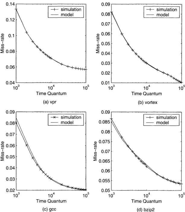
The results of the cache model and simulations are shown in Figure 2-5 in cases when a process starts its time quantum with an empty cache. Four benchmarks from SPEC CPU200 [14], which are vpr, vortex, gcc and bzip2, are tested. The cache is 32-KB fully-associative cache with a block size of 32 Bytes. The miss-rate of a process is plotted as a function of the length of a time quantum. In the figure, the simulation results at several time quanta are also shown. The figure shows a good agreement between the model's estimation and the simulation result.

As inputs to the cache model, the average miss-rate of each process has been obtained from simulations. Each process has been simulated for 25 million memory references, and the miss-rates of the process for various cache size have been recorded. The simulation results were also obtained by simulating benchmarks for 25 million memory references with flushing a cache every T memory references. As the result shows, the average miss-rate works very well.

10 Time Quantum (a) vpr 104 Time Quantum (C) gcc 10 2) C,, 0.09 0.08 0.07 0.06 0.05 0.04 0.03 0.02 10 10 Time Quantum (b) vortex Cl, U) 0.09 0.085 0.08 0.075 0.07 0.065 0.06 0.055 0.05 105 103 -+- simulation - model -I-sm lto -4+ simulation -- model -104 Time Quantum (d) bzip2

Figure 2-5: The result of the cache model for cache flushing cases. (a) vpr. (c) gcc. (d) bzip. 0.14 0.12 - +I- simulation - model 0.1 C, 0.08 0.06 0.04' 10 3 ->- simulation model 0.09 0.08) 0.07 0.06 0.05 a, CO, 0.04 0.03 0.02 10 105 10 (b) vortex.

0.042 800 simulation vortex 0.041 - approximation 700 -- vpr - - model 0.04600 -0.039 -0- 500-tZ0.038 4 C4Q 400 -0.037 -! 300 0.036 _E <200 -0.035 -20 0.034 -100~ 0.033 0' 0 5 10 0 2 4 6

Time Quantum x 104 Time Quantum x 104

Figure 2-6: The result of the cache model when two processes (vpr, vortex) are sharing a cache (32 KB fully-associative). (a) the overall miss-rate. (b) the initial amount of data xi(0).

2.4.2

General Cases

Figure 2-6 shows the result of the cache model when two processes are sharing a cache. The two benchmarks are vpr and vortex from SPEC CPU2000, and the cache is a 32-KB fully-associative cache with 32-B blocks. The overall miss-rates are shown in Figure 2-6 (a). As shown in the figure, the miss-rate estimated by the model shows a good agreement with the results of the simulations.

The figure also shows an interesting fact that a certain range of time quanta could be very problematic for cache performance. For short time quanta, the overall miss-rate is relatively small. For very long time quanta, context switches do not matter since a process spends most time in the steady state. However, medium time quanta could severely degrade cache miss-rates as shown in the figure. This problem occurs when a time quantum is long enough to pollute the cache but not long enough to compensate for the misses caused by context switches. The problem becomes clear in

0.07 1 _r__ simulation .. approximation - - model 0.065-(D 0.06-0.055 - 0.05-0.045'' 0 1 2 3 4 5 6 7 8 9 10 Time Quantum X 10 4

Figure 2-7: The overall miss-rate when four processes (vpr, vortex, gcc, bzip2) are sharing a cache (32K, fully-associative).

Figure 2-6 (b). The figure shows the amount of data left in the cache at the beginning of a time quantum. Comparing Figure 2-6 (a) and (b), we can see that the problem occurs when the initial amount of data rapidly decreases.

The error caused by our approximation (Equation 2.22) method can be seen in Figure 2-6. In the approximation, we assume that the data left in the cache at the beginning of a time quantum are all in the MRU region of the cache. In reality, however, the data left in the cache could be the LRU cache block and get replaced before other process' blocks in the cache, although the current process' data are likely to be accessed in the time quantum. As a result, the approximated miss-rate is lower than the simulation result when the initial amount of data is not zero.

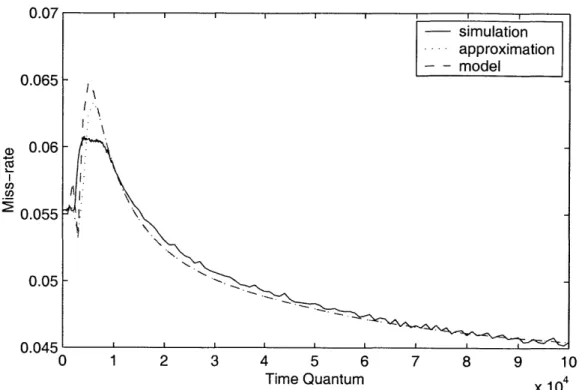
A four-process case is also modeled in Figure 2-7. Two more benchmarks, gcc

and bzip2, from SPEC CPU2000 [14] are added to vpr and vortex, and the same cache configuration is used as the two process case. The figure also shows a very close

agreement between the miss-rate estimated by the cache model and the miss-rate from simulations. The problematic time quanta and the effect of the approximation have changed. Since there are more processes polluting the cache compared to the two process case, a process experiences an empty cache in shorter time quanta. As a result, the problematic time quanta become shorter. On the other hand, the effect of the approximation is less harmful in this case. This is because the error in one process' miss-rate becomes less important as we have more processes.

Chapter 3

Cache Partitioning Based on the

Model

In this chapter, we discuss optimal cache partitioning for multiple processes running on one shared cache. The discussion is mainly based on the analytical cache model presented in Chapter 2, and the presented partition is optimal in a sense that it minimizes the overall miss-rate of the cache.

The discussion in the chapter is based on similar assumptions as the analytical model. First, the memory reference characteristic of each process is assumed to be given by a miss-rate curve that is a function of cache size. To incorporate the effect of dynamically changing behavior of a process, we assume that the memory reference pattern of a process in each time quantum is specified by a separate miss-rate curve. Therefore, each process has a set of miss-rate curves, one for each time quantum. Within a time quantum, we assume that one miss-rate curve is sufficient to represent a process.

Second, caches are assumed to be fully-associative. Although most real caches are set-associative caches, it is much easier to understand the tradeoffs of cache partition-ing uspartition-ing a simple fully-associative model rather than a complicated set-associative model. Also, since a set-associative cache is a group of fully-associative caches, the optimal partition could be obtained by applying a fully-associative partition for each set.

Cache Partition at TQ(2, 1)

D 2 D (2,1)

X(2,1) X (',2

Amount 1 Amount of Process 2's

Data at this Point Data at this Point

Process 1 Process 2 ... Process Process 1 Process 2 ...

STime

TQ(1,1) TQ(1,2)

Round 1

TQ(1,N) TQ(2,1) TQ(2,1)

Round 2

Figure 3-1: An example of a cache partition with N processes sharing a cache.

Finally, processes are assumed to be scheduled in a round-robin fashion. In this chapter, we use the term "the length of a time quantum" to mainly represent the number of memory references in a time quantum rather than a real time period.

3.1

Specifying a Partition

To study cache partitioning, we need a method to express the amount of data in a cache at a certain time as shown in Figure 3-1. The figure illustrates the execution of N processes with round-robin scheduling; we define the term round as one cycle of N process being executed. A round starts from Process 1 and ends with Process N. Using a round number (r) and a process number (p), TQ(r,p) represents Process p's time quantum in the rth round. Finally, we define X(rp) as the number of cache

blocks belonging to Process i at the beginning of TQ (r, p).

We specify a cache partition by dedicated areas and a shared area. The dedicated area of Process i is cache space that only Process i uses over different time quanta. If we define Dr as the size of Process i's dedicated area between TQ(r - 1, i) and

TQ(r, i), D' equals to X ri). For static partitions when memory reference patterns Start

do not change over time, we can ignore the round number and express Process i's dedicated area as Di.

The rest of the cache is called a shared area. A process brings in its data into the shared area during its own time quantum. After the time quantum, the process's blocks in this area are evicted by other processes. Therefore, a shared area can be thought of as additional cache space a process can use while its active. S(ri), the size of a shared area in TQ(r, i), can be written by

i N

S(ri)

P=1 P=i+1

where C is the cache size. The size of a shared area is expressed by S for static partitioning.

3.2

Optimal Partitioning Based on the Model

A cache partition can be evaluated by the transient cache model that is presented in Section 2.3.1. To estimate the number of misses for a process in a time quantum, the model needs the cache size (C), the initial amount of data (xj(0)), the number of memory references in a time quantum (Ti), and the miss-rate curve of the process

(m(x)).

of data xj(0) for each process. Therefore, we can estimate the total number of misses for a particular cache partition from the model.

From the definition of a dedicated area, Process i starts its time quantum TQ(r, i) with Dr cache blocks in a cache. In the cache model, the cache size C stands for the maximum number of blocks a certain process can use in its time quantum. Therefore, the effective cache size for Process i in time quantum TQ(r, i) is (D+S(ri)). For each time quantum TQ(r, i), a miss-rate curve (mr) and the number of memory reference

(T[) are assumed to be given as an input.

TQ(r, i) as follows:

missTQ(ri) = miss(m'(x), Ti, D', D' + S(r,'))

m (xi(t))dt (3.2)

mr(MIN[(M[ )-1(t + M[(Dr)), D. + S(r i)])dt

where dMir(x)/dx = mr(x) from Equation 2.11. In the equation, miss(m(x), T, D, C)

represents the number of misses for a time quantum with a miss-rate curve (m(W)), the length of the time quantum (T), the initial amount of data (D) and cache size (C). If we assume Process i terminates after Ri rounds of time quanta, the total number of misses can be written by

N Rp

total misses Z miss(r, p). (3.3)

p=1 r=1

In practical cases when processes execute for a long enough time, the number of time quanta Ri can be considered as infinite.

Note that this equation is based on two assumptions. First, the replacement policy assumed by the equation is slightly different from the LRU replacement policy. Our augmented LRU replacement policy replaces the dormant process' data in the shared area before starting to replace the executing process' data. Once dormant process' data are all replaced, our replacement policy is the same as the normal LRU replacement policy. The equation also assumes that the dedicated area of a process keeps the most recently used blocks of the process.

Since S(ri) is determined by D', the total number of misses (Equation 3.3) can be thought of as a function of D'. The optimal partition is achieved for a set of integer

Dr that minimizes Equation 3.3.

For a cache without prefetching, D' is always zero since the cache is empty when a process starts its execution for the first time. Also, Dr cannot be larger than Xr , the amount of Process i's data at the end of its past time quantum.

3.2.1

Estimation of Optimal Partitioning

Although we can evaluate a given cache partition, it is not an easy task to find the partition that minimizes the total number of misses. Since the size of a dedicated area can be different for each round, an infinite number of combinations are possible for a partition. Moreover, the optimal size of dedicated areas for a round is dependent on the size of dedicated areas for the next round. For example, consider the optimal value of Dr. Dr affects the number of misses in the r round (miss(r, 2)), which is also dependent on the size of Process 1's dedicated area in (r+1)h round. As a result, determining the optimal partition requires the comparison of an infinite number of combinations.

However, comparing all the combinations is intractable. This problem can be solved by breaking the dependency between different rounds. By assuming that the size of dedicated areas changes slowly, we can approximate the size of dedicated areas in the next round from the size of dedicated areas in the current round, D+l ~ D, which enables us to separate the partition of the current round from the partition of the next round.

The number of misses over one round that is affected by Dr can be written as follows from Equation 3.2.

p-1 N missD (Dr) = miss(mr, T, D, C - D+1 - D) p=1 _{q=1 q=p+1} N p-1 N + ~ miss(m-', T71 _{, D-, C- D-} Dq) p=i+1 q=1 q=p+1

Since we assumed that D+1 ~ Dr and the size of dedicated areas for the first round is given (D' = 0), we can determine the optimal value of D' round by round.

3.3

Tradeoffs in Cache Partitioning

In the previous section, we discussed a mathematical way to determine the optimal partition based on the analytical cache model. However, the discussion is mainly

based on the equations, and does not provide an intuitive understanding of cache partitioning. This section discusses the same optimal partitioning focusing on trade-offs in cache partitioning rather than a method to determine the optimal partition. For simplicity, the discussion in this section assumes one miss-rate curve per process and therefore static cache partitionig.

Cache partitioning can be thought of as allocating cache blocks among dedicated and shared areas. Each cache block can be used as either a dedicated area for one process or a shared area for all processes. Dedicated cache blocks can reduce inter-process conflicts and capacity misses for a inter-process. Shared cache blocks can reduce capacity misses for multiple processes. Unfortunately, there are only a fixed number of cache blocks. As a result, there is a tradeoff between (i) reducing inter-process conflicts and (ii) reducing capacity misses for one process and reducing capacity misses for multiple processes.

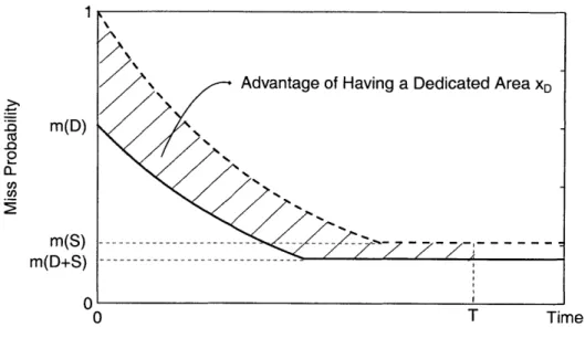
A dedicated area can improve the cache miss-rate of a process by reducing misses caused by either conflicts among processes or lack of cache space. Specifically, if data left in the dedicated area from past time quanta are accessed, we can avoid inter-process conflict misses that would have occurred without the dedicated area. A dedicated area also provides more cache space for the process, and may reduce capacity misses within a time quantum. As a result, a dedicated area can improve both transient and steady-state behavior of the process. However, the advantage of a dedicated area is limited to one process. Also, a shared area has the same benefit of reducing capacity misses.

The advantage of having a dedicated area is shown in Figure 3-2 based on the analytical cache model. The dashed line in the figure represents the probability of a miss at time t for a process without a dedicated area. Time 0 represents the beginning of a time quantum. Without a dedicated area, the process starts a time quantum with an empty cache, and therefore the miss probability starts from 1 and decreases as the cache is filled with more data. Once the process fills the entire shared area, the miss probability becomes a constant m(S), where S is the size of a shared area. Since time corresponds to the number of memory references, the area below the curve

1 m(D) Cn m(S) --- ---- -- m(D+S)---0 0 T Time

Figure 3-2: The advantage of having a dedicated area.

from time 0 to T represents the number of misses expected for the process without a dedicated area.

Now let us consider a case with a dedicated area D. Since the the amount of data at the beginning of a time quantum is D, the miss probability starts from a value

m(D) and flattens at m(D + S) as shown by the solid line in the figure. The area

below the solid line between time 0 and T shows the number of misses expected in this case. If m(D) is smaller than 1, the dedicated area improves the transient miss-rate of the process. If m(D + S) is smaller than m(S), the dedicated area improves the steady-state miss-rate of the process. Even though a dedicated area can improve both transient and steady-state miss-rates, the improvement of the transient miss-rate is the unique advantage of a dedicated area.

A larger shared area can reduce the number of capacity misses by allowing a

process to keep more data blocks while it is active. A process starts a time quantum with data in its dedicated area, and brings new data into the cache when it misses. The amount of the active process' data increases until both the dedicated area for the process and the shared area are full with its data. After that, the active process recycles the cache space it has. As a result, the size of shared area with the size of a

1

Advantage of Having a Larger Shared Area

-o -0 0 m(D+S1) --- -- -- - - -m (D +S 2) -0' 0 T Time

Figure 3-3: The advantage of having a larger shared area for a process.

dedicated area determines the maximum cache size a certain process can use. A larger shared area can increase cache space for all processes, and therefore can improve the steady-state miss-rate of all processes.

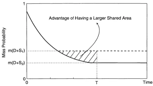
Figure 3-3 illustrates the advantage of having a larger shared area for a process. The dashed line represents the probability of a miss as a function of time with a shared area SI. Time 0 represents the beginning of a time quantum. The process' expected number of misses is the area below the curve from time 0 to T, where T is the length of a time quantum. The miss probability starts from a certain value and becomes a constant once both the dedicated and shared area are full. A cache with a larger shared area S2 can store more data and therefore the steady-state miss probability becomes m(D + S2) as represented by a solid line in the figure. A larger shared area can reduce the number of misses if m(D + S2) is smaller than m(D + S1). The

improvement can be significant if the time quantum is long and therefore a process stays in a steady-state for a long time. On the other hand, a larger shared area may not improve the miss-rate at all if the process does not reach a steady-state. Since a shared area is for all processes, the advantage of having a larger shared area is the sum of advantages for all the processes.

2048 1536 _{a Dedicated (P1)} 1024 512 0 0 512 1024 1536 2048 Cache Size

Figure 3-4: Optimal cache partitioning for various cache sizes.

For small caches, the advantage of increasing a shared area usually outweighs the advantage of increasing a dedicated area. If a cache is small, reloading cache blocks only takes a relatively short period compared to the length of time quantum, and therefore steady-state cache behavior dominates. At the same time, the working set for a process is likely to be larger than the cache, which means that more cache space can actually improve the steady-state miss-rate of the process. As a result, the optimal partitioning is to allocate the whole cache as a shared area as shown in Figure 3-4. The figure shows optimal cache partitioning for various cache sizes when two identical processes are running with a time quantum of ten thousand memory references. The miss-rate curve of processes, m(x), is assumed to be e- 0 1 .

Assuming the same time quanta and processes, a shared area becomes less im-portant for larger caches. As the size of the shared area increases, a steady-state miss-rate becomes less important since a process starts to spend more time to refill the shared area. Also, the marginal gain of having a larger cache usually decreases as a process has larger usable cache space (a shared area and a dedicated area). Once the processes are unlikely to be helped by having more shared cache blocks, it is better to

4no 6M, 300 2040, 10 10 10 10 10 X 104 5 5X 10,4 5X10 T2 0 0 T1 1 0 0 T1 (a) (b)

Figure 3-5: Optimal cache partitioning for various time quanta.(a) The amount of Process l's dedicated area. (b) The amount of shared area.

use those blocks as dedicated ones. For very large caches that can hold the working sets for all the processes, it is optimal to allocate the whole cache to dedicated areas so that no process experiences any inter-process conflict.

The length of time quanta also affects optimal partitioning. Generally, longer time quanta make a shared area more important. As a time quantum for a process becomes longer, a steady-state miss-rate becomes more important since the process is likely to spend more time in a steady-state for a given cache space. As a result, the process needs more cache space while it is active unless it already has large enough space to keep all of its data.

An example of optimal partitioning for various time quanta is shown in Figure 3-5. The figure shows the optimal amount of a dedicated area for Process 1 and a shared area when two identical processes running on a cache of size 512 blocks. Time quanta of two processes as the number of references, T and T2, are shown in x-axis and y-axis

respectively. The miss-rate curve of the processes, m(x), is assumed to be e-0 Ol. As discussed above, the figure shows that a shared area should be larger for longer

400600 4000 0.101 0.05 0.05 b2 0 0 bl b2 0 0 bl (a) )

Figure 3-6: Optimal cache partitioning for various miss-rate curves. (a) The amount of Process l's dedicated area. (b) The amount of shared area.

time quanta. If both time quanta are short, the majority of cache blocks are used as dedicated ones since processes are not likely to grow within a time quantum. In the case of long time quanta, the whole cache is used as a shared area.

Finally, the characteristics of processes affect optimal partitioning. Generally, processes with large working sets need a large shared area and vice versa. For example, if processes are streaming applications, having a large shared area may not improve the performance at all even though time quanta are long. But if processes have a random memory access pattern with a large working set, having a larger cache usually improves the performance. In that case, it may make sense to allocate a larger shared area.

Figure 3-6 shows optimal partitioning between two processes with various miss-rate curves when the cache size is 512 blocks and the length of a time quantum is 10000 memory references. The miss-rate curve of Process i, mi(x), is assumed to be

e-i. If a process has a large bi, the miss-rate curve drops rapidly and the size of the