Asymptotically unbiased inference for a dynamic panel model with fixed effects when both n and T are large

Digitized

by

the

Internet

Archive

in

2011

with

funding

from

Boston

Library

Consortium

IVIember

Libraries

Massachusetts

Institute

of

Technology

Department

of

Economics

Working Paper

Series

ASYMPTOTICALLY UNBIASED

INFERENCE

FOR

A

DYNAMIC

PANEL

MODEL

WITH

FIXED EFFECTS

WHEN

BOTH/7

AND

T-ARE

LARGE

Jinyong

Hahn

Guido

Kuersteiner

Working

Paper

01

-17

December

2000

Room

E52-251

50

Memorial

Drive

Cambridge,

MA

021

42

This

paper can be

downloaded

without

charge

from

the

Social

Science Research Network

Paper

Collection

at

MASSACHUSEHS

INSTITUTE

OF

TECHNOLOGY

AUG

1

5

2001

Massachusetts

Institute

of

Technology

Department

of

Economics

Working Paper

Series

ASYMPTOTICALLY

UNBIASED INFERENCE

FOR

A

DYNAMIC

PANEL

MODEL

WITH

FIXED EFFECTS

WHEN

BOTH/7

AND

TARE

LARGE

Jinyong

Hahn

Guido

Kuersteiner

Working

Paper

01-17

December

2000

Room

E52-251

50

Memorial

Drive

Cambridge,

MA

02142

This

paper can be downloaded

without

charge from

the

Social

Science

Research Network Paper

Collection

at

As3miptotically

Unbiased

Inference

for

a

D3rQaimc Panel

Model

with

Fixed

Effects

When

Both

n

and

T

are

Large

Jinyong

Hahn

Guido

Kuersteiner

Brown

University

MIT

December, 2000

Acknowledgement:

Helpful

comments

by

Joshua

Angrist,

Gary

Chamberlain, Jerry

Hausman,

Dale Jorgenson,

Tony

Lancaster,

Whitney

Newey, and

participants of seminars at

BC/BU,

Harvard/MIT,

Johns Hopkins

University, Pennsylvania State University, Rice University,

Texas

A

&

M.

University of

Virginia, 1998

CEME

Conference,

and

1999

Econometric

Society

North American Winter Meeting

are appreciated.

Abstract

We

consider a

dynamic

panel

AR(1)

model

with fixed effects

when

both

n

and

T

are large.

Under

the

"T

fixed

n

large" asymptotic approximation, the

maximum

likelihood estimator is

known

to

be

inconsistent

due

tothe well-knownincidental peirameterproblem.

We

consider

an

alternativeasymptotic approximation

where

n

and

T

grow

atthe

same

rate. Itis

shown

that,although the

MLE

isasymptotically biased, a relatively simple fix to the

MLE

results in an asymptotically unbiased estimator.

The

bias corrected

MLE

is

shown

to

be

asymptoticallyefficient

by

a

Hajek

type convolution theorem.

Key

Words:

dynamic

Panel,

VAR,

largen-large

T

asymptotics,bias correction, efficiency

1

Introduction

In this paper,

we

consider estimation ofthe autoregressive

parameter

ofa

dynamic

panel data

model

withfixedeffects.

The

model

hasadditive individualtimeinvariant intercepts (fixed effects)alongwith a

parameter

common

toevery individual.

The

total

number

ofparameters isthereforeequaltothe

number

of individuals plusthedimensionofthe

common

parameter, say

K.

When

the

number

of individuals (n)

islargerelativetothetimeseriesdimension (T), a

maximum

likelihoodestimatorofall

n

+

X

parameters

would

lead to inconsistent estimates of the

common

parameter

ofinterest.

This

isthe well-known

inci-dental

parameter

problem.^ Inconsistencyofthe

MLE

under

T

fixed

n

large asymptotics lead toa focus

on

instrumentalvariables estimation intherecent literature.

Most

instrumental variablesestimatorsare

atleastpartly

based on

the intuition thatfirstdifferencing yieldsa

model

freeof fixedeffects.^ Despiteits

appeal as a procedure

which

avoids the incidental

parameter

problem, the instrumental variables based procedure isproblematic as ageneral principle to deal

with

potentially nonlinear panel

models

because ofits inherent reliance

on

first differencing.

Except

for a small

number

of cases

where

conditioning

on

some

sufficient statistic eliminates fixed effects, there does not

seem

to exist

any

general strategy even

for potentially nonlinear panel models.

In this paper,

we

develop such a general strategy

by

considering an alternative asymptotic

approxi-mation

where both

n

and

T

are large.

We

analyze properties ofthe

MLE

under

this approximation. It

is

shown

that the

MLE

is consistent

and

asymptotically normal, although it is not centered at the true value ofthe parameter.

The

noncentrality

parameter under

our alternative asymptotic approximation implicitly captures bias of order

O

{T~^),

which

can

be

viewed as an alternative

form

ofthe incidental

parameter

problem.

We

develop a bias-corrected estimator

by examining

the noncentrality parameter.

Our

strategy can

be

potentially replicated in nonlinear panel models, although analytic derivations for

nonlinear

models

are expected to be

much

more

involved

than

in linear

dynamic

panel models.

We

can

in principle iterate our strategy to eliminate biases oforder

O

{T~^) or

O

{T~^), although

we

do

not pursue such a routehere.

Having

removed

the asymptotic bias,

we

raise

an

efficiency question. Is the bias-corrected

MLE

asymptotically efficient

among

the class of all reasonable estimators? In order to assess efficiency,

we

deriveaHajek-type convolution theorem,

and

show

thatthe asymptoticdistribution of the bias-corrected

MLE

is equal tothe

minimal

distribution inthe convolution theorem.

Our

alternative asymptotic approximation is expected to

be

of practical relevance if

T

is not too

small

compared

to

n

as is the case for

example

in cross-country studies.^

The

properties of

dynamic

panel

models

are usually discussedunder theimplicit

assumption

that

T

issmall

and

n

is largerelying

on

T

fixed

n

largeasymptotics.

Such

asymptotics

seem

quite natural

when

T

is indeed very small

compared

ton. In cases

where

T

and

n

areof

comparable

size

we

expect our

approximation

to

be

more

accurate.

'See

Neyman

and Scott (1948) for generaldiscussion on the incidental parameter problem, and Nickell (1981) for its

implication in theparticular lineardynamicpanel model ofinterest.

^Fordiscussion ofvariousinstrumentalvariablesestimatorsandmomentrestrictions, seeHoltz-Eakin,Newey, and Rosen

(1988),ArellanoandBond (1992). Chamberlain (1992),

Ahn

and Schmidt (1995), Arellanoand Bover (199.5). Bhmdell and Bond (1995), and Hahn (1997).

^Inter-country comparison studiesseems to bea reasonable application forsuch perspective. See Islam (1095) and/or

It should be

emphasized

that

some

of the results in Sections 3 are independently

found

by

Alvarez

and

Arellano (1998).

They

derived basically the

same

result (and

more)

for the

MLE

and

other

IV

estimators

under

the

assumption

that (i) the initial observation has a stationary distribution,

and

(ii)

the fbced effects are normally distributed

with

zero

mean.

Although

our result is derived

under

slightly

more

general assumptions in that

we do

not

impose

such conditions, this difference should

be

regarded

as

mere

technicality.

The more

fundamental

difference isthat they

were

concerned with the

comparison

ofvariousestimators for

dynamic

panel

data

models whereas

we

are concerned with biascorrection

and

efficiency. Phillips

and

Moon

(1999) recently considered a panel

model where both

T

and

n

are large.

They

consideredasymptoticproperties of

OLS

estimators fora panelcointegrating relation

when

both

T

and

n

go toinfinity. This

paper

differs

from

theirswith respect tothe

assumption

that

<

lim

n/T <

oo

whereas

they

assume

hm

n/T

=

as

n,T

-^ oo. It is

shown

in Section 3 that the asymptotic bias of

the

MLE

(OLS)

is proportional to

^njT.

Phillips

and

Moon

(1999)

showed

that the

OLS

estimator

is consistent

and

asymptotically

normal

with zero

mean.

Although

their setup is different

from

ours

in the sense that their regressor is

assumed

to

be

nonstationary, it is plausible that their asymptotic unbiasedness of

OLS

critically hinges

on

the

assumption

that lim

njT

=

0.

2

Bias

Corrected

MLE

for

Panel

VAR

with Fixed

Effects

Inthis section,

we

considerestimationoftheautoregressive

parameter

^o ina

dynamic

panel

model

with

fixed effects

3/it

=

ai

+

yif-i^o

+ 4.

i=

1,.-. ,n; <

=

1,... ,r, (1)

where yn

is an

m-dimensional

vector

and

e\^ is i.i.d. normal.

We

establish the asymptotic distribution

ofthe

OLS

estimator

(MLE)

for _^o

under

the alternative asymptotics,

and

develop

an

estimator free

of (asymptotic) bias.

We

go

on

to argue that the bias corrected

MLE

is efficient using a

Hajek

type convolution theorem,

and

provide

an

intuitive explanation ofefficiency

by

considering the limit ofthe

Cramer-Rao

lower

bound.

Finally,

we

point out that the asymptotic distribution ofthebias corrected

MLE

is robust to nonnormality

by

presenting

an

asymptotic analysis for a

model where

z\^ violates the normality assumption.

We

leave theefficiency analysis of

models

with

nonnormal

innovations forfuture research.

Model

(1)

may

be understood as a parametric completion of the univariate

dynamic

panel

AR(1)

model

with additional regressors. If

we

write

yn

=

{Y^i,X[^J^^ , then the first

component

of the

model

(1)

can be

rewritten as

yit

=

Ci+/3o-y,t-i+7oX,<+e,,,

2

=

1,... ,n; f

=

1,...

,T

(2)

where

Ci

and

(/3q,7o)'denote thefirst

component

of q,

and

thefirst

column

of9'^. Thisimpliesthat,

under

thespecial circumstances

where

Xj( followsa first order

VAR,

we

can regard

model

(1) as a completion

of

model

(2).

Under

this interpretation,

model

(1)

encompasses

panel

models

withfurther regressorssuch

as (2).

Even

more

generally,

model

(1) can

be

parametrized tobethereduced

form

ofa

dynamic

simultaneous

requires

imposing

blockwise zero

and

identity restrictions

on

^o- It is well-known that

MLE

reducesto blockwise

OLS

as long therestrictions are block recursive.

Even

though

we

do

not spellout thedetails of this interpretation of our

model

it is clear that extending our results to this

more

general case is

straightforwEird .

If

we

assume en

is i.i.d. overt

and

i,

and

has azero

mean

multivariate

normal

distribution, then the

MLE

(fixed effects

estimator/OLS)

takes the

form

where

yi

=

_^

X]t=iVittVi-

—

^ St=i

Vu-i-

We

examine

properties

oiG under

potentialnonnormalityof

£it under thealternativeasymptotics. Ifthe innovations en arenot

normal

then theresultingestimator 9 isa

pseudo-MLE,

and

does

no

longer possessthe efficiency properties ofthe exact

MLE.

Forthis reason

we

impose

the additional

assumption

ofnormality for

om

discussion ofasymptoticefficiency later in this

section.

We

impose

the following conditions:

Condition

1 (i) en is i.i.d. acrossi

and

strictly stationary in t for eachi,

E

\eu\

=

for alli

and

t,

E\eue'J

=

Ql{t==

s}; (ii)

<

lim^

=

_p

<

oo; (in)

lim„^oo^o

=

O/ °-^d (iv)

_^

^."1=1 \y^o?

=

0(1)

The

innovations e,( are uncorrelated but not independent. Their higher order

dependence

allows for

conditionaJ heteroskedasticity. In order to

be

able to establish central limit

theorems

for our estimators

and

tojustify covariancematrix estimation

we

needto

impose

additional restrictionson thedistribution

oftheinnovations.

The

dependence

islimited

by

afourth order

cumulant summability

restriction slightly

strongerthan in

Andrews

(1991).

These

conditions could berelatedto

more

primitivemixing conditions

on

the underlying en as

shown

in Andrews(1991).

We

defineu*^

=

Yl'jLo^o^a-j-Condition

2

oo

y^

|cumj,,...,j, (7i*,,,eit2."*(3'^io)|

<

oo

Vi

andji,...,jk

S

{1,...,to} .

tl,*2.<3

=

—oo

Inthe

same way

as

Andrews

(1991),

we

define zn

s

(/igiu*(_j)£n

and impose an

additionaleighthorder

moment

restriction

on

eu,

which

takes the

form

ofafourthorder

cumulant summability

condition

on

zu.

Condition

3

oo

|cumj,,...,j^{zH,,zn2,Zit3,Zio)\

<

oo Vz"

ond

ji,...,jt € {l,...,m}.

oo

'j,'2.'3=-00

Renicirk

1 In Condition 1, our requirement that

<

lim:^

=

p

<

oo corresponds to the choice of a

particular set ofasymptotic sequences.

The

choice of these sequences is guided by the desire to obtain asymptotic approximations that

mimic

certain

moments

of the finite

sample

distribution,

m

our case

the

mean

ofthe estimator.

Bekker

(1994. _P-661) argues that the choice ofa particular sequence can be

justified by its ability to "generate acceptable approximations of knoivn distributional properties of related

In ourcase it

seems

most

appropriateto investigate the properties of the score relatedto the

dynamic

panel model. After concentrating out the fixed effects,

we

are lead to consider the normalized score process

S^t

=

-7^

Y^=i

St=i

{^

®

[Vit-i

—Vi-))

(^a —£i)- In the appendix,

we show

that^

SnT

-^

S

under

the alternative asymptotics with

n/T

-^ _p, where

S

has a

normal

distribution with

mean

equal

to

—y/p{I

<SiI

—

{I

®

_^o))~ vec(O). Clearly,

under

fixed

T

large

n

asymptotics the score process has

an

explosive

mean

leading to the inconsistency result.

The

exact finite sam,ple bias for the score is given by

E

[5„rl

= -^^7^T-l

Y^^,

Y.]=o (^

®

^0)vec(fi).

The term

-^pT'^

_YJ=i

_EJ=o

_(^

®

_{^0) vec}(fi)

converges to —y/p{I'S>I

—

(/®

^o))~^

vec(n)

=

E[S]

by the Toeplitz

lemma

as

T

—

> 00,

and

is closer

to

E[S\

for small values of6q. In other

words

our asymptotic sequencepreserves the

mean

ofthe score process in the lim.it.

The

_form

_ofthe approximation error also

may

explain simulationfindings indicating that the approximation improves for larger values of

T

and

deteriorates with6 getting closer to the unit

circle.

Our

asymptotics

may

also be understood as

an

attempt to capture the bias of the score of order

O

(T~^)

.

We

show

in theappendixthatthescoreprocessis wellapproximated bya process, saySil^-p,^ such

that

E

[S:,^]

=

-

yf

i

_YlLi

_Ej=o

{l

®

_{^0) vec}(fi).^

Because

the

term

^

_J2j=i

_Ej=o

_(^

®

_{^0) vec}(fi) is oforder

O

(1), the approximate

mean

ofthenormalizedscoreprocess canbe elicitedonly by considering the alternative approximation where

n

and

T

grow

to infinity at the

same

rate.

The

mean

of the score process that our asymptotics captures

may

also be identified as the bias of the score

up

to

0(T~^).

Because

the score

—^=sSnT

is approximated by -^^S^j-,

and

because

E

SnT

nT

'tt

T

4-1

E

E

(^

®

^0) vec (Q)

=

-(-(/ ®

/

-

(/

®

Oo))-'vec(fi)

+

o₍₁₎₎ ,

t=lj=0

we

may

understand

_-^

(/(g)7

-

(/

®

^o))~^ vec(Jl) as the bias ofthe score oforder

O

{T~^).

Remctrk

2

Condition 2 _{implies Yl'jL-oa}ICovj-j.fcj {zit,Zit-j)\

<

00, because

Covk,,k2{zit,Zrt-3)

=

cum,,,..,,^ _{{u*t_-^,eu,u*t_i_^,£it-j)}

+

Covi^^i^ (u*t_],u*t_i-j)^ovi^j^ {eit,ett-j)

+

Cov^j,,, {u*^_^,Cit_j)Covi^^i^

«<_i_j,eit)

,

where

ki

=

lim

+

12

+

1

and

k2

=

l3ni

+

I4

+

I vnthli, ...,14

e

{0,1,...,m}. In this sense our Condition 2

is stronger thanthefirstpart of

Assumption

A

in

Andrews

(1991). Condition

3

is identical tothe second part of

Assumption

A

in

Andrews

(1991).

Remark

3

In the special case _{where Eu} is iid across i

and

t Conditions

2

and

3 are equivalent to

E

A3)\

_<

00 for allj

where

e\j is thej-th element in e^t- See

Lemma

1 in

Appendix

A.

We

show

below that the

MLE

9 is consistent, but

v^nTvec

io

-

9'q\ is not centered at zero:

''Lemma6 in Appendix A.

^The exactdefinition ofS*j. is given in (12) in Appendix A.

Theorem

1 Let

ya

be generated by (1).

Under

Conditions 1, 2

and

3,

we

have

V^vec

(e

-9'^-*N

_{(- Vp(/}

®T)-^

{1

®

I

-

[I

®

0o))~'^vec(fi)

,(/

®

T)"'

(fi

®

T +

/C)(7

®

T)"^)

,

whereT

=

_{Q+^o«^o+^o«}

_(^o)'+-'

',

^

=

E^-oc^(«'0)'

^

(^i-^z)

=

E

[(/®

<,,_i)

e„,4,

(/

®<,_i)]

—

jE[£'itifit2]

®

-^_["i^o'^iol' '^"'^_"it

—

_{Yl'jLo^o^it-j-}

U

in addition allthe innovations

eu

areindependent foralli

and

t then

VnTvec

(o

-

e'^]

^

M

(-^{I

®

T)"^

(7

®

/

-

(/

®

^o))"' vec(fi),

O

®

T"^)

.

Under

our alternative asymptotic sequence the

MLE

is therefore consistent but has a hmiting

dis-tribution that is not centered at zero.

The

non-centrahty

parameter

results

from

correlation

between

the averaged error terms

and

the regressors j/it-i-

Because

averaging takes place for each individual

the estimated

sample

means

do

not converge to constants fast

enough

to eliminate their effect

on

the limiting distribution.

Under

our asymptotics the convergence is

however

fast

enough

to eliminate the inconsistency

problem

found forfixed

T

large

n

asymptotic approximations.

When

the irmovations are not iid then the limiting distribution is affected

by

higher order

moments

reflecting theconditional heteroskedasticity in the data.

The

limiting covariance matrix

n<SiT

+

Kl can

alsobe expressedaslimT""^

_Ylut2=-T

^

[{^

®

"iti-i)^J'i^it2 (-^

®

_"itj-i)]

Standard

tools forconsistent

and

optimal estimation of

fi®T

+

/C werediscussedin

Andrews

(1991).

Under

ourconditions the results

of

Andrews

are directly applicable.

Our

theorem

1 roughly predicts that

yec(9

-e'o)^Af(-^{I®T)-^I®I-{I®eo)r'yec{n),^{I®T)-'{n®T

+

JC){I®rr'Y

Therefore, the noncentrality-parameter -i/p(7

®

T)~^

{J

®

I

-

{I

®

do))'^ vec(fi) can be viewed as a device tocapture bias oforder

up

to

O

[T~

^

) .

Our

bias corrected

MLE

is given

by

-1" 7( /2' vec I 9 f

;^

EE

(2^''-'

-

2/,-) [yu-i

-

2/.-)' j i=l t=l , (3) I'here n

T

^^^EE(2/''-i-y-)(y"-i-^-)''

and

vec(n)

=

(707-(^®^))vec(f).

(4)

i=a <=i

Theorem

2

Let

_yn

hegenerated by (1). Then,

under

Conditions 1, 2

and

3,

we

have

V^wecCe

-e'o]

-^7V('o,(7®T)~^(n®T +

/C)(/(8.T)"M.

// in addition all the innovations Su are independent for alli

and

t then

We

now

show

that thebias-corrected

MLE

is asymptotically efficient.

We

do

so

by showing

that the asymptoticdistribution ofthebias corrected

MLE

is 'minimal' in thesense of

a

Hajek

type convolution

theorem/

We

show

that the asymptotic distribution of

any

reasonable estimator can

be

written as a

convolutionofthe'minimal'

normal

distribution

and

some

otherarbitrary distribution. In this sense, the

bias-corrected

MLE

can be

understoodto

be

asymptotically efficient.

Condition

4

(i)

_en

~

Af{0,9.) i.i.d.; (ii)

<

lim^

=

p

<

oo; (Hi)

lim„_«,

_^o

=

0/ «"<^ 0'")

i Er=i

\y^o\'

=

o

(1)

and

1 Er=i

l".l'

=

0(1).

In order to discuss efficiency

we

naturally

have

toguarantee that 6is theexact

MLE.

Forthis reason

we

impose

the additional requirementof

normal

innovations incondition (4).

Theorem

3

Let

y^

he generated by (1).

Suppose

that Condition (4) is satisfied. Then, the asymptotic

distribution of

any

regular _{estimator ofvec{9o) cannot} be

more

concentrated i/ianA/" (O,

O®

T~^).

Proof.

See

Appendix

C.3.

It should

be emphasized

that

Theorem

3 initselfdoes not say anything

about

theattainability ofthe

bound

0(g)

T~^

.

The

asymptotic variance

bound

itprovidesis a lower

bound

ofthe asymptotic variances

ofregular estimators.

On

the other hand, itis notclear

whether

such a

bound

is attainable.

Comparison

with

Theorem

2 leads us to conclude that the

bound

is attained by the bias corrected

MLE

as long as the innovations

en

are iid Gaussian.

Corollary

1

Under

Condition 4, the bias corrected

MLE

6 is asymptotically efficient.

3

Application

to

Univariate

Dynamic

Panel

Model

with Fixed

Effects

In this section,

we

apply

Theorems

1

and

2 in the previous section to the univariate stationary panel

AR(1) model

with fixed effects

y^t

=

Q^

+

9Qyit_x+eit, I

=

1,... ,n; t

=

1,... ,r. ₍₅₎

We

also consider estimation offixed effects q; in the univariate contexts. Finally,

we

examine

how

the

resultchanges

under

the unitroot. Itturnsout that thedistribution of the

MLE

isquite sensitive tosuch

aspecificationchange.

As

such,

we

expect that ourbias corrected estimator will not

be

(approximately) unbiased

under

a unitroot.

We

first apply

Theorems

1

and

2 to the univariate case. Obviously, Condition 4

would

now

read

(i) e^t

~

7V(0,fi) i.i.d.; (ii)

<

limf

=

p

<

go; (iii) |6»o|

<

1;

and

(iv)

_{^ Er=i}

2/^)

=

0{\) and

i Er=i

"?

=

d

(1).

Note

that the

MLE

(OLS)

is given

by

-

_{_}

_:^

Er=i

ELi

ivit

-

Vi) (j/^t-l

-

y^-)

7^ Er=i Er=i

[y^t-i

-Vi-)

Applying

(3)

and

(4) to the univariatemodel,

we

obtain

^^^(^ttiy^^-^'-y^y

_nT

K l=\ t=\

^

" 1 "

^

1 -1 1=1 1=\

where

\ 1=1 t=l /

Therefore,our bias correctedestimator isgiven

by

Because

T

=

_„; in the univariatecase,

we

can conclude

from

Theorem

2 that

At^^-^o)

-^M{o,i-el)

Prom

Theorem

3,

we

can alsoconclude that9 isefficient

under

thealternativeasymptotics

where

n,T

^>

CO at the

same

rate.

Our

theoretical result

may

be

related to Kiviet's (1995) result.

He

derived

an

expression of

some

approximate

biasofthe

MLE,

which

depends on

the

unknown

parameter

valuesincluding ^o-

He

showed

by

simulation that the infeasihle bias-corrected

MLE,

based

on

such

knowledge

of^o, has

much more

desirable finite

sample

properties than various instrumental variable type estimators.

Because

his bias correction

depends

on

the

unknown

parameter

value ^o, feasible implementation appears to require a

preliminary estimator of^o-

He

considered instrumental variable type estimators as preliminary

esti-mators

in his simulation study, but he failed to

produce

a theory for the corresponding estimator.

Our

bias corrected estimator,

which

does not require a preliminary estimator of6o,

may

be

understood as

an

implementable

version of Kiviet's estimator. Also, our convolution

theorem

may

be

understood as a

formalization ofhis simulationresult.

We

now

consider estimation offixed effects q^. Recently,

Geweke

and

Keane

(1996),

Chamberlain

and Hirano

(1997),

and

Hirano (1998)

examined

predictive aspects of the

dynamic

panel

model

from

a Bayesian perspective.

FVom

a Frequentist perspective, prediction requires estimation of imlividiial

specific intercept terms.

We

argue that intercept estimation is asymptotically unbiased to begin with,

separately Einalyzed even for thepurpose of prediction.

Observe

that the

MLE

ofa, is given

by

T

-,

T

1

T

1

ai

_J2

{yn

-

hit-?)

=

"i

+

_^

^

£,t

-

p

-

^o)

_^

_j]

vit-i. (7)

(=] t=\ t=i

so that

(1)

1

^

Because

-t

_XltLi^i* converges in distribution to

N

(O, CTq) as

T

-> oo, the

MLE

is asymptotically

unbiased. Furthermore,

we

have

1 "^

VT'(aj

-

Qi)

=

—=

^£i«

+

Op(1) ,

V-^ _t=i

where

Sj denotes the estimator of Oi obtained

by

replacing the

MLE

6 in (7)

by

the bias corrected

estimator 9. It follows that

more

efficient estimation _{of ^o} does not affect the estimation ofa^.

We

now

consider the nonstationary case

where

^o

=

1-

We

first consider a simple

dynamic

panel

model

with aunit root,

where

individual specific intercepts are all equal tozero but the econometrician

does not

know

that.

The

econometrician thereforeestimatesfixed effects along with 9.

Theorem

4 Suppose that (i) en

~

M

(O,a^) i.i.d; (ii) ai

=

0; (Hi) Oq

=

1;

and

(iv)

n,T

-^ oo.^

We

then have

V^T'{i-e„.^)-.^f{o.'j)

Proof.

See

Appendix

D.l.

One

obviousimplication of

Theorem

4 isthatthe bias correctionforthestationary caseisnotexpected

to

work

under the unit root. In order tounderstand the intuition, it is useful to note that

Theorem

4 roughlypredicts that

which

indicates thatthebiasonly

depends on

T. For example,

Theorem

4 roughlypredictsthatthe

MLE

is centered

around

_| if

T =

5.

The

bias correction for the stationary

model

critically hinges

on

the fact

that the

rough

bias in afinite

sample

is a function of

n

and

T,

and

hence, is not expected to

be

robust

tothe unit rootspecification.

We

now

consider the case

where

individual specific intercepts are nonzero,

and

the econometrician estimates

them

along with 9.

Theorem

5 Suppose that (i) £,t

~

N

(0,0^) i.i.d; (n)Jim

^

YTi^i

«?

>

0; (ni) 9q

=

1;

and

(iv)lim

_y^

exists.

We

then have

^ '

\ lim- > _i of Inn

-

_> 'No particular rateon the growthofn and

T

is imposed.

Proof.

See

Appendix

D.2.

Although

Theorem

5 shares the

same

feature as

Theorem

1 as far as the asymptotic bias being

proportional to _{lim .^y,} it is quite clear that thebias correction for thestationary case does not

work

because the asymptotic bias

under

the unit root

depends

on

lim

-

_Y!d=i**?•

4

Monte

Carlo

We

conduct a small

Monte

Carloexperimentto evaluatethe accuracyofour asymptotic approximations to the small

sample

distribution of the

MLE

and

bias corrected

MLE.

We

generate samples

from

the

model

Vit

=

cti

+

Ooyu-i

+

Sit

where

yit

£

M, ^o

€

{0,.3, .6,.9}, a^

~

^(0,1)

independent across i,

and e^

~

TV

(0,1) independent

acrossi

and

t.

We

generate q^

and

su such that theyare independent ofeachother.

We

chose yio\Oi

~

M

(yr^'

^r-P'

''

)-

The

effective

sample

sizes

we

consider are

n

=

{100,200}

and

T

G

{5, 10,20}.^ For

each

sample

ofsize

n

and

T

we compute

thebiascorrected

MLE

6 based

on

the formulation (6).

We

also

compute

the usual

GMM

estimator

9gmm

based

on

the first differences

Vrt

-Vzt-l

=

OoiVit-l

-yit-2)+£it

using past levels {yio,--- ,J/it-2) as instrvunents. In order to avoid the complexity of weight matrix

estimation,

we

considered Arellano

and

Dover's (1995) modification.^°

Finite

sample

properties of

both

estimators obtained

by

5000

Monte

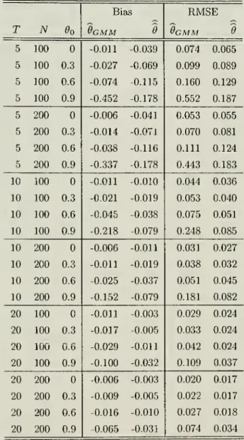
Carlo runs are

summarized

in

Table 1.

We

can see that

both

estimators have

some

bias problems. Unfortunately, our bias corrected estimator does not completely

remove

the bias. This suggests that

an

even

more

careful small

sample

analysis based

on

higher order expansions of the distribution

might

be needed

to account for the entire

bias.

On

the other hand, the efficiency of

measured by

the root

mean

squared error

(RMSE)

often

dominates

that ofthe

GMM

estimator,suggestingthatourcrude higher order asymptotics

and

therelated

convolution

theorem

provided a reasonable prediction

about

the efficiencyofthebias-corrected

MLE.

5

SumniEiry

Inthispaper,

we

considered a

dynamic

panel

model

withfixed effects

where

n

and

T

are of the

same

order ofmagnitude.

We

developed a

method

to

remove

the asymptotic biasof

MLE,

and showed

that such a biascorrected

MLE

is asymptoticallyefficient in the sense that itsasymptoticvariance equals that ofthe

limit ofthe

Cramer-Rao

lower

bound.

Our

simulation results

compare

our efficient bias corrected

MLE

to

more

conventional

GMM

estimators. It turns out that our estimator has

comparable

bias properties

and

often

dominates

the

GMM

estimator in terms of

mean

squared error loss for the

sample

sizes that

we

think our procedure is

most

appropriate for.

'A moreextensiveMonte Carloresults are availablefrom authorsupon request.

'"Arellanoand Bover(1995) proposedtouse themomentrestrictionsobtained by Helmerl'stransforiiialionofthesameset

One

advantageofusingbiascorrected

MLE

asthe guidingprincipleforconstructing estimatorsisthat

itcan

more

naturally

be extended

tononlinearmodels.

GMM

estimators

on

the other

hand

ultimatelyrely

on

transformations suchasfirstdifferencingor similaraveraging techniquesto

remove

theindividual fixed

effects.

Such

transformations are inherentlylinear in nature

and

therefore notsuited forgeneralizations to a nonlinearcontext.

Our

techniquecaninprinciple

be

generalized to

remove

biasofhigher order

than

T~^

by

repeating the alternativeasymptotic

approximation

scheme

for

an

appropriately rescaled version of the bias corrected estimator.

We

are planningtopursue this avenueinfuture research.

Our

bias corrected

MLE

is notexpected to

be

asymptotically unbiased

under

aunit root.

We

leave

development

ofabias corrected estimatorrobust to nonstationarity tofuture research.

Appendix

A

Proof

of

Theorem

1

Theorem

1 isestablished

by combining

Lemmas

6

and

7 below.

Note

that

Vit

=

elViO

+

{/

-

^0)~' (1

-

^o) a.

+

^0~'^il

+

C^f.2

+

•••

+

Sit. (9)

In the stationary case

where

lim„6q

=

0,

we

work

with the stationary approximation to

_{yu which}

is

given

by

oo

y*=(/-0o)"

ai+<„

t>0.

The

vectorized representation ofthe

OLS

estimator for 6q is given

by

(10)

(11)

vec

[o-o',)

/ n

T

^®

_\JZYl(y''-^

-j/,-)(2/2*-i

-Vi-)'

\t=i t=i

J2J2i^®

(j/,t-l

-

y^-)) {£^t

-

£,)

1=1 t=l

where

fj

=

J;

_J^ff

if.

We

definethejoint

cumulant

next. Let.^

=

{£,-[,

_,(,k)

^ K*"

and

e

=

(sll^',...,ell''')

is the joint characteristic

func-where

e^' is the j-th element of £t, then <Ajj,...jt,t,,...,«t

(0

=

E

e'^

^

tion with corresponding

cumulant

generating function In</>jj

..j^,<j_ ..^t^ (0-

The

joint v-th order

cross-cumulant

function is 0Vj

+

...

+

Vk cumj,,...jt (£(!,---etj

dC,'--dCk'

ln'^j...>.,(i,....u(^) i=o

where

Vi are nonnegativeintegers v\

+

...

+

Vk

=

v.

Lemma

1 Lete,( beiid acrossi

and

t

and

E

Conditions 2

and

3 hold.

-U)

_<

oo.

Assume

Conditions4 (H) - (i"^)hold.

Then

Proof.

Available

upon

request

from

the authors.

Lemma

2 Let

_yu

hegenerated by (1). Also, let

uT

₌₁

t=l

Then under

Conditions 1, 2

and

3

T

"-' _{-=i (=1}

(12)

Proof. Because

_Yli=i {^

®

Vi-) i^n

~

^i)

—

*^'

^"^

itsuffices to prove that

n

T

(

=

1

v"J

_i=it=i

vnJ

_{,^j (^j}

From

(9), (10),

and

(11),

we

obtain

yu

=

y^

+

9^(y^o

-

<o)

-

(^

-

^o)~^^o«i-

We

may

therefore write

=EE(^®2/.t-l)(e^t-?.)-^EE(/®y;t-l)(f^t-^o

=

_{EE(^®^W(^^'-^o}

(13)

2=1 «=1

nT^

_{1 t=i}

n

r

-

(7

-

00)-^

-J=^

Vy:(/®^^a^)

(e,t

-e.)

(14)

^ 2

=

1f=l

-4fEE(^®^o<o)(^^t-^0-

(15)

^

1=1 t=l

We

analyze (13) first.

By

assumption, its expectationis zero.

Because

of

independence

of£i(

and

yio,

we

have

/

T

_\

^

,

T

T

Var

_Q^

(/

®

^^j/io) (e.t

-

?z)

=

E

(^

®

^o^'o)

"

(^

®

^'O^o)

-

_t

E

E

(^

®

^o^.o)

^

(7

®

y^o^o')

-i

=

l t=l s=l

from which

itfollowsthat

vec

Var

_{'^J2f2{l^9ly.o){eu-eA}

=

T-^

(7(g)7(g)7

®

7

-

(7

O

e^o)

®

(7

®

fi'o))"^ _((/

®

6*0)

®

(/

®

^0)

-

{{I

®

6»o)

®

(7

O

610))^+')

X

vec

(

n"^

E

(^

®

^'0^

^

(-^

®

^'O^ )

1=1

-r-2

₍₇

®

(7

-

^0)"' (»o

-

<+'))

®

(/

®

(/

-

^o)~' (^0

-

^r'))

vec (

n-^

^

(/

®

y.o)

^

(/

®

2/-o)

=

o(l).

1=1

It therefore follows that (13) is Op(l). In the

same way

it follows that (14) is Op(l).

We

turn to the analysis of(15).

Because

ofindependenceof

_{£u and}

u*q,

we

cansee that ithas a

mean

equalto zero,

and

vec

_{v3siY;^{i®eiu:o)en}

J2

((^

®

^0)

®

U®do))

vec

(E

[(7

®

<o)f.*,4,

{J®0])

,(2=1

T

^

((7

®

<>)

®

(^

®

_^oO)

(^

_{h'.4J ®}

E

[<o<o]

+

^0

(«i.'2)).

ii,(2=l

T

(l,'2=l

where

the matrix /Co(ii,i2) contains elements of the

form

cum^^^.j^ {u*Q,u*Q,£it^,£uJ.

The

sum

over thefirst

term

then can

be

expressed as

T

Y^

((/

®

^o)

®

U

®

^o))vec[n

®

£«o<o)]

=

(/

®

/

®

/

®

/

-

((/

®

^o)

®

(/

®

^o)))"' t=i

X

_(((/

_®

_^o)

_®

(/

®

^o))

-

((/

®

^o)

®

(/

®

^o))^+') vec [0

®

E

_[<o<o]]•

The

second

term

is

bounded

by

T

T

E

ll(^®^oO®(^®^o')||l|vecX;oUi,<2)||<sup||vec/Co(ti,i2)||

^

_||(/

®

^^0

®

(^

®

^olll

<

oo

Togetherthese results

imply

that

Var

(-^

^,"=1

_TI=i

(^

®

_^o<o)

^^')

=

o(!)

Next

consider

VarK^(/®^^<o)^.

v(=i

T-2

E

_{((^®^o)®(-^®^o^))^ec£;[(/®<o)£.<34.U®<o)]}

(,,..,(4=1

<

_||(/

®

(/

-

^0_') (^0

-

^r'))

®

(/

®

(/

-

^0_') (^0

-

^r'))

r

r-'vec[0^£;[u*oM*o]]+r"^

E

vec^o(«3,'4)

(/

®

(/

-

9o') [eo

-

e^'))

®

(/ (/

-

^0

') (^0

-

^r'))

X

M|T-^vec[n®£;[<o<^]]||+T-2

^

Hvec/Co (f3,«4)ll

)

=0{T-'),

which shows

that

Var

(-?=

Yl'i=-i13^=1 (^

®

^o"io)

^0 ~

''(^)- ^^^ therefore followsthat (15)is Op(1)

Lemma

3 Let

_ya

he generated by (1).

Under

Conditions 1, 2

and

3,

-. n

T

Proof.

We

have n

T

nT

E

=

1

_EE(^®<')^'

"

^

i=] (=1

"

_{;);EE^K/®<*)^"}

nTT

nl

(=1 5=1

T

I 77 1

T

(-1

By

the usual result on Cesaro averages,

we

have

_^

_{Y.i=\ IZj=o(-^}

_®

^0)

=

{I

®

i

-

[1

®

Oo))

+

o(l). Therefore,

1 "

^EE(^®<')^'

=

^>(I®I

-{I®

e„)r'

vcc (S^)

+

o₍₁)

.

We

also

have

T

=

E

T

oo -l

T

oo tl,..,t4

=

lji,J2= t],..,t4

=

_lil,J2=0

T

<l,.-,t4

=

l <l,.-,t4

=

l

where

/C («i,i2,t3,(4) is a matrix containing elements of the

form

cumj^^„,j, _{("*iii^it2i"it3)^it4)-}

This

leads to

^^

(

=

1 _/ (,,t3

=

l(2

=

1«4

=

1

T

OO min(T,(3-j])

+

^EE

E

{i®o{^){Q^n')[i^er^^-'^)

T

+

T3

A^

tl,..,ti=

T

,..,«4

=

1

The

first

term

on the right is

O

(T

^) because

T

t-i

T

^

^

(/

®

el'-'^)

=

^

(/

®

/

-

/

®

_^o)"'

{l®I-I<^9*o')=

0{T).

t,=1*4=1 f,=l

second

term

is

O

{T~^) because

The

vec iin{T,(3-ji+l)

Y^

(l®

%'

) (f^

®

0') (/

®

^^0=) J2=0 OO OO

EE||(^®^oO®(^®^)

i,=072=

E

_

J)=0 J2=0 (/(g»/)

®

(/

®

fi'j^) II ||vec{J^

®

n')ll

=

O

(1) ji=072=0

Finally, the third

term

is

O

{T'"^) because

^

_II(j,..,(4=icumj,,..,j, [u*n^,£u^,ul^^,€u,)

=

O

(T"^) by

the

cumulant

summability assumption.

Lemma

4

Assume

et is a sequence ofindependent, identically distributed

random

vectors with

E

[et]

=

forallt.

Then

cum^, ,_^^ (ej,,_...,£t^)

=

unlessii

=

t2

=

=

tk-Inthiscase

we

define

cum

[ji,

,jk)

=

Lemma

5 Let Conditions 1, 2

and 3

be satisfied.

Then

where

IC=Y:Z-.o^it^O)

and)C{t,j2)

=

E[{l^uU^_,)eitAt,

(/

®

<_0]

--^

h<,4j®-E[tx>^^].

// in addition all the innovations en are independentfor alli

and

t then

Proof.

We

need tocheck the generalized Lindeberg Feller condition forjoint asymptotic normality

asin

Theorem

2of Phillips

and

Moon

(1999).

A

sufficient conditionforthe

theorem

tohold isthatforall

ieW^

suchthat

fE

=

1 itfollows

E

{-^EUni®u;,_,)su)

<

oo uniformlyini

and

T. Letting Zit

=

a

(i w*(_i)Sit

and

noting that

E

[zi(]

=

we

consider

1

^

1 -^

^

£'[z,t,z,t2Z,(3Z,tJ

=

_—

_J

^

[Cov(z,(,,z.(JCov(z,(3,z,(J

+

Cov(z,t,,Zi(3)Cov(z,t2,Zi«4)] J'2 (,,. .(4

=

1 t],..(4

=

1

T

"^

r2

E

|Cov(z,t,,z,(JCov(zi,2,Zi(3)

+

cum(za,,Zit2,Zit3.Zi(4)l> (l,...(4=l

where

Gov

(za,z,,)

-

(!E

_[(/

®

<(_!)

e,iz\, [l

®

u*,_^

i

=

f

vec

[E

_{K,_i4])}

vec

[E

[<_j4])'£

+

f

£

[£.,4]

® E

[u*,_,n^:_,] i

m

— 1 il, •J4=0

=

+

f

(n

E

_{K_i<,i])}

M

{<

=

5} Tn— 1

+

^^

^j3m+ji+l^J4m+j2+l'^^nnj),...j4 _{(Uij_i,£ii,}W;3_2,Cisj.

ji,...,J4=0

Using

these results

we

deduce

that

1

^

^

E

•E'lz^tiZif^ZitjZifJ

r

m-l

+

6(f

_{(0®£[<<_lW';_l])£)}

_h^

E E

^j3m+j,+ l^j4m+J2+

lCUmj,

;4 K(-l.^.('"*s-l'^.s) '.5=1 J1,...,J4=0

T

m-l

+

3

-

^ ^

_£j3m+ji+l^j4Tn+j2+lCUmj,,...,j„ «(_],£,(,<,_i,C,-s) \ (,S=1ji,...j4= 1

^

m^ / 1 \

+^

n

Yi

in^^O'''""^'

J4(z.',.z.'2-z.'3.z-'..) 'i. '..=l7l J.i=l \^=1 15

where

the terms involving higher order cumulants are

_^

_{Xlt,s=i ^^™Ji.}•:74(''^r«-i'^i<'''*rs-i'^«) ""

^W

and

_E?i,...t4=icum^,, ..,jJz„,Zit,Zit3ZitJ

=

0{T)

independent oiiJi,...,J4- This

shows

that

T

(l,...t4

=

l

uniformly ini

and

T. Finally consider 21

(;^|:('«<.-.)^..'

=

_^

^

£((;»»•,_, )e,.4 ('»"."-)!

t,s=]

T

t,5=l

n^T

+

ic+oii). (,s=l t,s=l

where

/C

=

_{X;^=-oo''^(«i,0).}

Note

that vec

[E

[<t_ie',,])vec

{E

[<_i4])

=

for all t

and

s

and

that

T

Em=i ^

If^'^'tsl

®

-E^[":<-i":s-i]

=

T

Er=i

£^l^.t^y

®

^

Nt-i<t'-i]

= «

® T

by

strict stationarity.

The

last line of the display follows

by

Cesaro

summability

and

stationarity.

The

second part of the

theorem

follows from

Lemma

(4) which impliesthat /C(ii,f2)

=

for all ii

and

i2-n

T

=

_{E E}

(^

®

(2/^'-i

-

_y-))

(^'*

-

^') -"

-^ (-^/^(^

®

-^

-

(^

®

^°))~'^^^ (^)'

"

® ^

+

^)

Lemma

6 Let y,t be generated by (1).

Under

Conditions 1,

2 and

3,

n

T

Proof.

The

result then follows

from

Lemmas

2, 3,

and

5.

Lemma

7 Letyu he generated by (1).

Under

Conditions 1, 2

and 3

n T

nT

;^

E E

(j^-'-i

- ^-)

(y^'-i

-

y^-)'

=

^

_[(y'*-i

-

_^y^^-i) (y'*-i

-

^y:*-i)']

+

op(i)

= t

₊

o^(i).

i=] (=1

Proof.

Available

upon

request from the authors.

B

Proof

of

Theorem

2

We

have

nr

vec

(^

-0',^^

^

®

_f;^

E E

(^"-^

-

_^-)

(y-'-i

-

y^-)'] 1=1 (=1

^\\

-1 16

Because

vec (T)

=

(7

-

(^o

®

do)) ^_vec(fi),

_and

₆

=

9o

+

Oj,_(1),

we

have

W^

(/

®

/

-

(/

®

?))

"'

vec (fi)

= v^

(7

®

7

-

(/

®

flo))"' vec (Q)

+

Op₍₁₎. ₍₁₈₎

Combining

with

Lemma

6,

we

obtain

1

n

T

I

—

J

;^EE

(^

_®

{yit-l-y^-))

{su

-^i)

+

J^

(/®

/

-

(7®?))"

vec

(n)

-iA^(0,(fi®T

+

/C)).

The

conclusionfollows

by

using

Lemma

7.

C

Proof

of

Theorem

3

C.l

Framework

For the discussion

and

derivation of theasymptotic variance

bound,

we

adopt the

same

framework

as in van der Vaart

and

Wellner (1996, p. 412). For this purpose,

we

discuss

some

oftheir notation. Let 77

be a linear subspace 77 ofa Hilbert space withinner product (•,)

and

norm

||||,

and

let Pn^h denote a

probability

measure on

a measurable space {A!n,An)- Consider estimating a

parameter «„

(h) based

on

an

observation with law Pn,h-

Now,

let {A/j :

h €

77}

be

the "iso-Gaussian process" with zero

mean

and

covariance function

E[Ah^Ah^]

=

(/ii,/i2)-

We

say that the sequence

{Xn,An,Pn,h)

is asymptotically

normal

if

]og^

=

A„,.-i||/zf

for stochastic processes {A„,ft : /i e 77} such that /\n,h converges weakly to A/, marginally under

P„_o-Now,

considerthesequence ofparameters «;„{h) belongingto a

Banach

space

B, which

is regular in the sense that r„(«„ (h)

-

k„ (0))

—

> k{k) for every /i

6

77 for a continuous, linear

map

k

:

H

-^

B

and

certainlinear

maps

rn :

B

-^ B.

A

sequence ofestimators

t„

is defined to

be

regular ifr„(t„

-

«;„ (h))

converges

weakly

to the

same

measure

L, say, regardless ofh.

The bound

ofthe asymptotic variance of a regular estimator can

be

found from the following

theorem due

to van der Vaart

and

Wellner (1996,

Theorem

3.11.2):

Theorem

6

Let thesequence (A'„,^„,P„,h :

h

£

H)

beasymptotically

normal and

thesequence of

param-eters Kn {h)

and

estimatorst„ be regular.

Then

the limit distribution

L

ofthe sequence r„ (t„

-

k„(ft))

equals the distribution of a

sum

G

+

W

ofindependent, tight, Borel measurable

random

elements in

B

such that

b*G

~

A^(0, ||k*6*||), for everyb* e

B'

. Here, k :

B*

^

H

is the adjoint ofk.

It can

be

seen that

G

provides us with the

minimal

asymptotic distribution for any regular estimator. If

G

happens

to be

normal

with

mean

zero, then

we

can say that itsasymptotic variance is the asymptotic

variance

bound.

We

show

that our setup iscovered

by

the preceding theorem. Ignoringirrelevant constants, thejoint

likeHhood ofthe

model

(1) is given

by

£

=

^logdet(*)-iX^^

trace

(4'Z,,K,e)),

(19)

i=l t=l

where

Zu

{a^,9)

=

_[yu

-

a^

-

_{d'yn-i) [yu}

-on-

9'yit-i)',

and

^ =

Q~^.

We

will localize the

parame-ter. Let

a

denote the sequence (Qi,a2,.. .

).

We

will attachsubscript todenote the 'truth'.

We

will

localizethe

parameter

around

the 'truth', so that 6

=

9 {n)

=

9o

+

-^^^^

'J'

= ^

(n)

=

'I'o

+

:y=f*:

and

a = a

(n)

s

ao

+

-^o-

Let h

=

(a,6,

$

j,

and

let

H

denote a set of

all possible values of fQ,^,

$

j

.

Let Pn^h denote thejoint probability

under parameters

characterized

by

h.

Theorems

7, 8,

and

9 in the next subsection establishes that, under Pn,o,

we

have

dPn,h _, 1

dPnfi

log3^=^n,;.-^i|A„,,f+Op(l),

n

T

^ n

T

where

A„,h

=

A„

(a,9,^^

converges

weakly

(under Pn,o) to A/j

~

A^

(0,\\h\\ _|. Here, \\h\\

=

{h,h),

and

(^(5i,?i,$i) ,

(52,^2,^2))

=

ivec(^2)'vec(fi)vec(n)'vec($i)

+vec(52)'(*®T^)vecp)

+

_£-

_^E"H*«-+

(vec(^£m^i|:a,5',jj

(*

®

(/

-

^')">ec

(^'2)

+

_{(^^^(nl^ooiE"^"2i))}

(*®(/-0-')vecp)

+

(vec(?2))'

(*®(/-6')"^

(„''H^~E"''*0

(^-^')~

l^ecf^i).

(20)

Inother words, the sequence (P„,/, : h E

H)

is asymptoticallynormal.

In order to adapt

Theorem

6 to our problem,

we

consider estimation ofthe "parameter" «„{h)

=

«;„ (a,0,ij*

j

=

9o+^^^

=

9,

which

isregularbecause r„ (k„(/i)

-

«„(0))

=

rn-l=9

=

9forr^

=

v'nT':

We

may

write

yfnT

{Kn(h)

-

k„ (0))

^

k{h)

for /t(/i)

s

k (a,^,

*

j

=

9.

We

restrict our attention to

regular estimators t„ of 9 such that the asymptotic distribution of

y/WT

[t^

—

Kn

(h))

=

VriT

{Tn

—

9)

C.2

Technical

Lemmas

In thissubsection,

we

omit the subscripts in 9o,^o,

and

ao

in orderto simplify notation.

We

have n

T

log-T^

=

—

logdetU'

+

-^=^)

-

log

det*

+

-VV

trace

(*Zit(a„0))

-

_^

y"

V

trace

( (

* +

-7=*

)

Zn

(a^

+

-^Q„e

+

-^e)]

Because

Za

{ai,9)

=

eu^'it

and

en

~

A/^(0,fi)

under

P„_o,

we

can write

=

.^1

+

02

+

(^3

+

<^4

+

05. (21) rp / 1 \ T^ 1 Tl I t)-,

=

—

logdet(

* +

^=^1

-

^logdet*

==

V

Vc',*ft(.

-. n

T

I

^

1 (=1 * i—1 (=1 1 "

^

/

where

i=l (=1 n

T

_

I

2nTylnT

.^j ^^^ n

T

_

I "4 rl t=l

Lemma

8

Under

_P^fi,

we

have n

T

-^

f^^trace

{^

{sue'u

-^))-\

(trace

(*-^*))'

+

o(l) .

'

2^nT

_{^^, ,^,}

Proof.

Follows from

nT

logdet

_(*

+

-^1'

I

-^logdet*

=

^!^trace(*-^*)

--

(trace

(*

'*))

+o{l),

2v"2"

_{,^j ,^j} . , -

^v..-,=1 t=i

Lemma

9

Under

P„

o, ^4

—

»A/" (O,ip^),

where

1 " 2 " -'

ip'^

=

lira

-

y

a'*a,

+

lim

-

V

a'*6' (/

-

6»)"^ a^

n—

>oo

_n

•'^

—

'

Ti—>oo

_n

^

—

'

(^*?'

t)

+

trace

leW

{I

-

9)"'^ i Jiirn^

-

^

a^a[

j (/

-

6')''^

j

+

trace|

Proof. Write

Apply

the

same

reasoning as in the proof of

Lemma

2 to the second

term on

the right

hand

side,

we

obtain

^ n

T

^

_

,

i=l t=l

Let _7i

=

a^

+

9{I

-6)

^

_a^

_and

Yrt

=

_7=^

_E"=i

{li

+

^<t-i)

*^it-

We

then

may

write ^4

=

E(_j

Vrt

+

Op(1). For each T, Yrt is amartingale differencesequence. Let aJ'^ denote theconditional

variance ofYti given {{uio,£iQ,... ,

eu-i)

,i

=

1,.. . ,n}.

We

then have

'Tt

—

^

(7,

+

^«*,_j)

*

(7i

+ Kt-i)

,

and

71

T

E4.

=

^

E^:*^.

+

;!

EE^:*^<-i

+ ;^

EE

Kvo'^'*^<-i-t=l i=l i=l t=l 1

=

1 t=l

It follows

by

standard

arguments

_{that Ylt=i'^Tt} ~^

^^

^^ probability.

By

strict stationarity,

we

have

E

[Y^t 1{\YTt\

>

£)]

=

^

[Y-^s 1_(l>Vs|

>

€)] Vs,<. Therefore, if

T

T

•.B [y^, 1_(lYTtl

>

e)]

=

^i?

[k2,• ₁

(lyrtl

>

0]

-

Ve

>

0, (22)

t=i

then

we

can use Billingsley (1995,

Theorem

35.12)

and

conclude that

n

T

^

E E

("^

+

^<'-i)'

*^^* _""

^

('^'^') i=\ t=\

Note

that

r.£[y2^.i(|yr<|>6)]

Because

1=1 \ * 1=1

>

%/Te

^

^=l !=1 L

0(1),

we

obtain (22) by

Dominated

Convergence.

Lemma

10

Under

Pn,o,

we

have(f>2

=

Op{l).

Proof.

By

Lemma

9,

we

have

(j)^

=

Op

(1), from

which

we

caneasily infer that 02

=

Op(1).

Lemma

11

Under

P„_o,

we

have 4>^

=

-^ip'^

+

Op(1).

Proof.

After applying a reasoningbasically the

same

as in theproofof

Lemma

2,

we

can obtain

^5

=

-^E^';^5,--if^^5:^?((/-^r^a.+<,_,)

1=1 i=l «=1

n

T

-^^T.J2{^^-^y''^i

+

<t-i)

'^e{{I

-9r'ai+u*^_,)+

_Opil). (23)

Itthereforesufficesto

show

n

T

^ n

T

^Y.tl

°i*^<t-i =op(i),

_^iiYl

((^

-^y' °0'

_^'*^<t-i

=

°p(1) ' i=l t=l i=l (=1

;^

E E

«<-i)'^'*^<t-i

=

trace (?'M'^

t)

+

o^(1) . i=\ t=l

All of

them

follow quite easily

from

characterization of

means

and

variances,

and

details are omitted.

Lemma

12

Under

Pnfl,

we

have<p^

=

Op(1).

Proof.

Followseasily with

Lemma

11.

Theorem

7

Under

Pn,o,

we

have

dPn,o

2VnT^^

V ^

VnT-^j^^jV

^

-

i

trace

((*-^$)Vi^X:"^*"'-^E"^*^(^-^r'"^

-

i

_trace

_f^'*^

_{t) -}

i

_trace

_j^'*^

_(/-

^)"'

(^E°'"0

i^

-

^Tj

+Op{l)-

(24)

Proof.

Follows

from

Lemmas

8, 9, 10, 11,

and

12.

Theorem

8

-77^EEt^^^<*(^''<t-"))

+

_{^EE(^'+^(^-^)"'"'+^<*-0'*'^'}

-^

AA

fo,

i

(trace

_(^*))^

+

V'^₎ ,

Proof.

It can

be

established

by

the

same

reasoning as in the proof of

Lemma

9,

and

details are

omitted.

Theorem

9

A^

(01,^1,$]

j

and

A„

(02,^2,

*2)

are jointly asymptotically

normal

with asymptotic

co-vanance

as in (20).

Proof.

Joint normality can be established by the

same

reasoning as in the proofof

Lemma

9,

and

details areomitted.

As

for the covariance, it can be inferred from the asymptotic variance in

Theorem

8

using the formula

Gov

{X.,

Y)

=

\ (Var(A'

+

K)

-

Var

(A) -

Var[Y)).

m

C.3

Proof

of

Theorem

3

We

may

write

n

T

n

T

n

T

=

vec

_{p') Ai„}

+

A2„

(5,

^)

.

Theorem

10

below

implies that the 'minimal' asymptotic distributionis

TV

I

J

£

Ai

A'j

j J

,

where

Ai

is the residual in the projection of

Ai

on

the linear space

spanned

by

•!

A2

(q,^j

>

Here,

Aj

and

A2

(a,

_^j

denote the 'limits' of

Ai„

and

A2n

(a,*].

Lemma

13

below

establishes that

/Aj,

A'A

=

^

(g)T. Therefore, the

minimum

variance ofestimation ofvec(^0) is given

by

the inverse of

*

®

T,

or

n®T-^

Theorem

10

Assume

that (P„,h :

h

G

H)

is asymptotically shift normal. Also, suppose that (i) h

=

{6,E), ho

=

(0,0); (ii)

k„

(/i)

=

_{„

=

_^o

+

J-6for

some

(,0

G

K; and

(iii) A;,

=

Aj

• 5

+

A2

(H).

FuHher

suppose that, with respect to the

norm

||-||, (iv) the m.apping

k

: (5,H)

—

> 5 25 continuous;

and

(v)

H

is

complete. Then, for every regularsequence ofestim,ators {t„},

we

have

rn{Tn

-

Hn{h)) -^

N

_Ue[i\i^Y'^

®W

for

some

W,

where

®

denotes convolution,

and

Ai

is the residual in the projection of

A^

on

{A2(H):(5,H)eH}."

Lemma

13 /Aj,

A'A

= ^

®

T.

Proof.

We

first establishthat

Ai

Ai

A2(l?i(/-0o)"'a,o)

A2

(^D^2 {I

-

Oo)-'

a,QJ

where, e'j denotes thejth

row

of 7^2,

and

£>j is

an

m

x

m

matrix such that vec{D'j)

=

Cj.

We

minimize

the

norm

of

e^Ai

- A2

(5,

*

j for eachj.

Prom

(20),

we

obtain

||e;Ai-A2(5,$)|p

_{= e;U®(7-0o)"'}

(„1H^^E"^°U

(^-^o)'')^^

n n

-2

lim

_{-y"5'*A(/-6io)"^Qz+}

lim

-^a.^a.

~\\2

+

Cj

_{*

®

T)

ej

+

_^

ftrace

_(^*))

"Thistheorem originallyappeared in Hahn (1998), butis reproduced hereforconvenience.

Therefore, the

minimum

of e^

Aj

- A2

(a,

_*^

is attained with

^ =

0,

and

a-

=

Dj

{I

-

9o) ^q^.

Observe

that the (j,fc)-element of

/Aj,

A'j\ is equal to

(e^Ai

-

A2

(d,

(/

-

^o)~'

Q„0)

,e'fcAi

- A2

(d^

(/

-

^0)"'

az,o))

.

After

some

tedious algebra,

we

can

show

that it isequal to e^('I'

®

T)

et. In otherwords,

/Ai,

A'A

=

D

Proofs

of

Theorems

4

and

5

Ignorethei subscript

whenever

obvious. Let

Ht

=

It

-

y^t^'ti V

=

{Vit ^Vt)',

V-

=

(j/o, ••

,yr-i)',

and

£

=

(ci,... .St)'

We

can write

_Yh=\

(^«

~^)

(j/*-i

-V-)

=

^'^tV-, and

J^Li

{vt-i

-V-)

=

y'_HTy--

Here, ^j' denotes T-dimensional

column

vector consisting of ones.

Note

that

y-

=

/1\

1 1 _yo

₊

/

\

1 2

_Q

₊

•

10

0-1 1

1111

^

=

i^itJ/0

+

?2ra

+

Are-vi

y

\T-i

)

Let _£>T

=

HtAx-

We

have Ht(,it

=

0,

and

hence, it follows that

Hry-

_{= U2T}

2~^^

)

"

"*"

^^^'

y'.Hry-

= U^t

-

^^t)

_f^T

"

_'^^^A

o?

+

2a£' _(^Czr

-

_^^^-j

₊

e'l^^Dx^

Inthe special case

where

a

=

0,

we

have

e'Ery-

=

e'Drs,

y'^Hry-

=

e'D'tDts.

Lemma

14

trace(IP^Z?,)

=

'-T^

-

1, trace

[[D'rDrf]

=

^T^

+

^T^

-

_^,

trace(£>^I?2^)

=

-^T2

+

_^,

trace (£>r

+

-Dt)

=

-'7^

+

1, trace

({Dt

+

J^r)^)

=

g^^

"^'^

~

_6' trace

((D.

+

D^)^)

=

-^T^

-

T

+

[

trace

((D.

+

D^)^)

=

^T"

+

^^^^

+

T

-

|

Lemma

15

/I5

n,T

—

00 23