Publisher’s version / Version de l'éditeur:
21st International Conference on Port and Ocean Engineering under Arctic Condition 2011 (Proceedings), 2012-01
READ THESE TERMS AND CONDITIONS CAREFULLY BEFORE USING THIS WEBSITE.
https://nrc-publications.canada.ca/eng/copyright
Vous avez des questions? Nous pouvons vous aider. Pour communiquer directement avec un auteur, consultez la
première page de la revue dans laquelle son article a été publié afin de trouver ses coordonnées. Si vous n’arrivez pas à les repérer, communiquez avec nous à [email protected].
Questions? Contact the NRC Publications Archive team at
[email protected]. If you wish to email the authors directly, please see the first page of the publication for their contact information.
NRC Publications Archive
Archives des publications du CNRC
This publication could be one of several versions: author’s original, accepted manuscript or the publisher’s version. / La version de cette publication peut être l’une des suivantes : la version prépublication de l’auteur, la version acceptée du manuscrit ou la version de l’éditeur.
Access and use of this website and the material on it are subject to the Terms and Conditions set forth at
Ship manoeuvring-in-ice modeling software OSIS-IHI
Lau, Michael
https://publications-cnrc.canada.ca/fra/droits
L’accès à ce site Web et l’utilisation de son contenu sont assujettis aux conditions présentées dans le site LISEZ CES CONDITIONS ATTENTIVEMENT AVANT D’UTILISER CE SITE WEB.
NRC Publications Record / Notice d'Archives des publications de CNRC:
https://nrc-publications.canada.ca/eng/view/object/?id=9e65fc57-f420-4018-8364-93fee3993425 https://publications-cnrc.canada.ca/fra/voir/objet/?id=9e65fc57-f420-4018-8364-93fee3993425
POAC11-138
SHIP MANOEUVRING-IN-ICE MODELING SOFTWARE
OSIS-IHI
Michael Lau
Institute for Ocean Technology, National Research Council of Canada, Canada
ABSTRACT
Software to model a ship manoeuvring in ice has been developed which will simulate the ice forces on a ship passing through a field of level ice and the resulting motions. OSIS-IHI (Ocean Structure Interaction Simulator – Ice-Hull Interaction) is an integration of two
separately-developed components. The first component is a static force solver that uses discrete-time motion data to calculate the resultant ice forces at a given point in time. The second component is an ordinary differential equation solver that produces dynamic motion data given a set of steering methods, such as propeller revolution and rudder angle deflection. It has been verified
extensively and used for client consulting work with success. The development and integration of both components is discussed, accompanied by preliminary verifications.
INTRODUCTION
Recently there has been an expansion of northern Arctic waterways, which will allow increased shipping and resource development in those regions. There is a potential for year-round shipping as global warming reduces the size of the polar ice sheets. However, the presence of ice will continue to be a factor, so as operations in northern waters expand there is an increased need to understand the motions of ships manoeuvring through ice fields. The effect of ice loads must be considered to ensure that ships are designed safely and economically, and that individuals have access to effective training simulators for operating ships in northern environments. New design technologies, including the double-acting tanker (DAT) and propellers mounted on steerable pods, are noted for their manoeuvring performance, but their performance in ice conditions has not yet been sufficiently modeled for prediction.
The National Research Council Institute for Ocean Technology (IOT) has been developing a model for predicting ship manoeuvring in ice. This has included model tests (Lau and Derradji-Aouat, 2004), numerical analysis (Lau, 2006) and analytical modeling (Liu et al., 2006; and Lau and Ni, 2009). These efforts have focussed on the resultant forces applied to a ship forced to manoeuvre in a simplified planar motion using a Planar Motion Mechanism. The accompanying analytical model IHI (Ice Hull Interaction) uses a static force solver and ignores force feedback. The static force solver uses discrete-time motion data to calculate the resultant ice forces at a given point in time. A description of this static force solver has been presented in addition to its verification with model scale data (Liu et al., 2006).
Recently, a ship manoeuvring in ice modeling software OSIS-IHI (Ocean Structure Interaction Simulator – Ice-Hull Interaction) was developed to simulate the ice forces on a ship passing through a field of level ice and the resulting motions. This software is an integration of two
POAC’11
Montréal, Canada
Proceedings of the 21st International Conference on
Port and Ocean Engineering under Arctic Conditions July 10-14, 2011 Montréal, Canada
separately developed components. The first component, IHI, is a static force solver that uses discrete-time motion data to calculate the resultant ice forces at a given point in time. The second component, OSIS, consists of an ordinary differential equation solver equipped with
hydrodynamic and propulsive force computation components that produces dynamic motion data given a set of steering methods, such as propeller revolution and rudder angle deflection. OSIS-IHI has been verified extensively and used for client consulting work with success. In this paper, the overall framework of the OSIS-IHI software and its theoretical basis are discussed.
Comparisons are made to self-propelled model- and full-scale data for model verification.
DESCRIPTION OF OSIS-IHI
OSIS was developed in Matlab as a platform for simulating dynamic ocean engineering models. The Matlab interface allows simulation creation, configuration, output analysis, and Audio Video Interweave (AVI) video generation. It was created as part of IOT’s commitment to performance modeling of ships and structures in ice. The purpose of OSIS is to provide a modular structure for the integration of different software models, allow execution of time domain simulations and be versatile enough to allow future upgrades and expansion.
The IHI module computes ice forces acting on the ship or model hull.
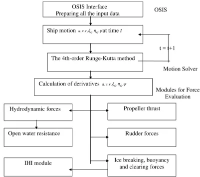
OSIS-IHI combines the ice forces computed by the IHI module with other external forces, i.e., hydrodynamic force, water resistance, rudder force and thrust, and employs momentum equations to solve for ship motion in the time domain. A
schematic of the computational algorithm is given in Figure 1.
The present version of OSIS-IHI is implemented as a stand-alone package,
equipped with a Graphical User’s Interface (GUI) and a toolbox for post-processing. The readers are referred to the OSIS-IHI user’s manual (Lau and Ni, 2009) for details
The 4th-order Runge-Kutta method Ship motion u,v,r,ξG,ηG,ψat time t OSIS Interface Preparing all the input data
Calculation of derivatives u,v,r,ξG,ηG,ψ
Hydrodynamic forces
Open water resistance
IHI module
Propeller thrust
Rudder forces
Ice breaking, buoyancy and clearing forces
OSIS
Motion Solver
Modules for Force Evaluation t = t+1
Captive and free run conditions
OSIS simulates motions in captive and free run conditions. For modeling captive motion, OSIS can be set to numerically simulate straight forward motion, pure sway, pure yaw, turning circles or any other arbitrary planar motions. The OSIS simulations available for modeling free motion are straight forward, spiral, zigzag, turning circle and any planar motion.
Captive run technology has already been extensively used to determine water resistance, and it is now being extended for use with ice conditions. The captive run conditions simulate the forces and moments when the ship is restricted to motion in a plane with the use of a Planar Motion Mechanism (PMM). A PMM imposes model motion in surge, sway and yaw and determines the response, i.e., ice load. Since the load response has no effect on future motion, the complications of force feedback can be neglected, providing a simplified case for initial static force model development and verification.
The IHI module has been validated using IOT in-house PMM model test data of the CCGS R-Class icebreaker, CCGS Icebreaker Terry Fox, USCGS Icebreaker Mackinaw and the new Korean Icebreaker Araon and found to be satisfactory (Lau and Ni, 2009).
Free run conditions are meant to simulate the ship motion when the ship is self-propelled to move in water or ice without any imposed captive motion. The environment in real operational
conditions may be complex, when ice, wind, waves and current are included. The motion can be controlled by the forces of a conventional rudder, thrusters or azimuthing podded propeller, etc. The control strategy can be as simple as setting fixed rudder deflection and constant propeller revolutions to make a turning motion. The ship motion can also be controlled by PID
(Proportional-Integral-Derivative) tragedy based on motion feedback to steering the ship on a pre-setting track using auto-pilot.
Ice force prediction module
A preliminary mathematical model was presented for ice-hull interactions by Lau and Derradji-Aouat (2004) and then further refined by Liu et al. (2006). This model, which has been adapted in software as the static force solver, considers the force exerted by ice on a ship’s hull as three independently calculated terms: the breaking force, the clearing force and the buoyancy force. Once calculated, all three terms are added together to define a global reactive ice force. The calculation of the terms presented by Liu et al. is summarized here.
The breaking force is determined from the contact area between the ship’s hull and the unbroken ice along with the mechanics of the ice itself. It considers both the flexural bending failure and the initial crushing failure as shown in Figure 2.
The buoyancy force is determined from the lift force applied by ice pieces covering the hull because of the difference in density between the ice and water. A simplified geometry represents the hull by a flat plate model, given in Figure 3. The volumes of ice on the sides of the hull are multiplied by the density difference between ice and water to give the buoyancy forces.
Figure 2. Ice-breaking model (Liu et al., 2006)
Figure 3. Hull geometry simplified for buoyancy force calculation (Liu et al., 2006)
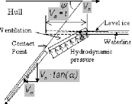
The clearing force considers a number of phenomena that make up the ice clearing process, shown in Figure 4. These are the viscous drag and inherent buoyancy of the rotating ice floes, forces caused by wave pressure and ventilation of the rotating ice floes, and inertial forces due to the ice acceleration. The inertial forces of the ice mass are calculated using the energy method, whereby the forces are those required to accelerate the ice floes from rest to the ship horizontal velocity divided by the cosine of the flare angle, Ψ . The wave pressure, viscous force and ventilation force use an added water mass coefficient. The computation algorithm is explained further in Liu et al. (2006).
The ice-ship interaction geometry is an essential aspect of the static force solver. In order to calculate the breaking and clearing terms of the ice force prediction module, the current contact area between the hull and the ice field is required (Liu et al, 2006). The hull waterline is defined as a line of discrete points based on the ship’s current position and orientation. The breaking and clearing forces are calculated for each waterline point, where applicable, and then summed to give a total breaking and clearing force. As the ship experiences motion, the location of the waterline is updated. Once the waterline has moved enough to have made contact with the ice field, the channel is expanded appropriately as ice is broken off. The expanding of the ice edge is displayed in Figure 5.
Figure 4. Ice piece turning and sliding schematic (Liu et al., 2006)
Figure 5. Schematic of the ice-hull contact in the numerical framework (Liu et al., 2006)
Motion solver
As noted, the captive run conditions form a simplified case since the ice load has no effect on ship motions. By ignoring force feedback, captive run simulations may impose motions that are
not physically possible. In order to realistically model free-run ship manoeuvring, a ship must be able to freely respond to the forces and moments imposed on it in order to properly evaluate its performance; hence, incorporating a force feedback algorithm with the force model is essential for a realistic motion calculation. The dynamic model makes use of force feedback to determine a ship’s motion. This allows for a more realistic representation of the ship’s manoeuvring
performance. Applied external forces, such as thrust and rudder force, together with the initial ship motions are inputs to the model. The motions are determined from the sum of the external and reactant forces, which are then used to re-calculate the ice-hull contacts and the associated ice-hull interaction forces.
This dynamic model is pseudo because the ice-hull interaction forces are assumed to be static, where the dynamic effects of ice, such as an elastic foundation, are ignored. The motions are calculated using an ordinary differential equation solver, which takes all applied forces and ice-hull interaction forces as inputs. The ice-ice-hull interaction forces are calculated using the same static force solver that performed the captive runs. These two components are combined to behave as a single feedback model. The ship manoeuvring motion is governed by
) (
)
(m−Xu u= Xuuu2 +Xpropeller +Xrudder +Xice +mvr+xGr2
ice rudder ic hydrodynam r G v v mx Y r Y Y Y Y m− ) +( − ) = + + ( (1) ice rudder ic hydrodynam r zz v G N v I N r N N N mx − ) +( − ) = + + (
where u, v and r are surge, sway and yaw, respectively, G(xG,0,0) is the ship weight center, m is the ship mass and Izzis the moment of inertia around the vertical axis in a body-fitted coordinate
system o-xyz.
The hydrodynamic forces Yhydrodynamic and Nhydrodynamicare
Yhydrodynamic Yvv Yr mU r Yvvv v Yrrr r Yvrrvr2 Yvvrv2r | | | | | | | | ) ( − + + + + + = Nhydrodynamic =Nvv+(Nr −mxGU)r+Nv|v|v|v|+Nr|r|r|r|+Nvrrvr2 +Nvvrv2r (2) and the ice force is determined by the IHI module.
In the current version, the resistance and propulsion are computed using the Holtrop method (1984) and the hydrodynamic forces on ship hull and rudder using Inouse method (1981). These ordinary differential equations for ship manoeuvring are solved numerically by the fourth-order Runge-Kutta method.
Resistance
The total resistance may be subdivided into seven components
ICE A TR B W APP F total R k R R R R R R R = (1+ 1)+ + + + + + (3) whereRFis the frictional resistance according to ITTC-1957 formula , (1 k+ 1) the form factor,
APP
R the appendage resistance, RW the wave resistance (neglected at low speed of ships in level ice), RB and RTR the additional pressure resistance of bulbous bow and due to transom immersion, respectively, R the model-ship correction resistance and A RICE is the ice resistance calculated by IHI.
The methods to calculate these components except RICEare given by Holtrop; RICE is developed
through a regression analysis of experimental data. Since the ship motion in ice is usually at low speed, more attention should be paid to the frictional resistance, form factor, appendage
resistance and ice resistance. Propulsion
For the conventional propeller the thrust is ) ( ) 1 ( p 2p 4 T p propeller t n D k J X = − ρ (4) where n is the propeller revolution, D the propeller diameter and the thrust coefficient p K is T
calculated from experiment data as a function of the advance ratio:
D n w u
Jp = (1− p)/ p (5)
where w is wake fraction and p t thrust reduction, both approximated from the ship particulars. p
The model measurement KT−Model(JP) should be corrected to obtain ship KT based on Reynolds number and propeller roughness according to the ITTC-1978 method.
The shaft power is determined from ) /( 1 1 0 η η ηR S p p E S t w P P − − = (6)
where P is the effective power, and the efficiencies are E ηR for relative-rotative efficiency, ηSfor shafting efficiency and η0for open water efficiency.
Hydrodynamic derivatives
The hydrodynamic derivatives used in Equations 1 and 2, Yv,Yr,Yv|v|,Yr|r|,Yvrr,Yvvr,
vvr vrr r r v v r v N N N N N
N , , ||, ||, , for viscous forces and Yv,Yr,Nv|,Nr,Xufor inertial forces (added mass) can be estimated by the Inouse method, which are based on principal dimensions of hull only. However, Inouse made the regression for model tests of oil tankers, container ships, ro-ro1 ships and dry cargo ships, not icebreakers, so it is more reliable to obtain hydrodynamic
derivatives from PMM experiment data for icebreaker models. Rudder force
The rudder located at positionx is deflected an angle δ δ to apply a control force F to the ship, N
resulting in surge Xrudder, sway force Yrudder and yaw moment Nrudder:
δ sin N rudder F X =− δ α ) cos 1 ( H N rudder F Y =− + (7) δ x Y Nrudder = rudder 1 roll-on, roll-off
Here αH is the ratio of induced force on the hull by the rudder over the rudder forceF , which is N
the lift force on the rudder as an airfoil
R R R N A V F α λ λ ρ sin 25 . 2 13 . 6 2 1 2 + = (8)
where the rudder area isAR, aspect ratioλ, effective inflow speed VR and effective attack angle R
α . The ship manoeuvring motion and propeller effect should be included in the expressions of both V and R αR of the rudder.
Example simulation
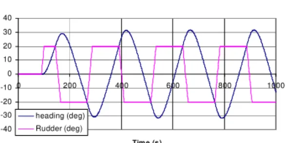
The zig-zag manoeuvre is a standard manoeuvring test in open water that is widely applied to stability analysis (Nomoto, 1957). A numerical simulation of zigzag manoeuvring motion in open water and ice for the USCG icebreaker Healy is shown here as an example to showcase OSIS’ motion simulation capability. Figure 6 and Figure 7 give the rudder angle and ship heading in ice and in open water, respectively, from the zigzag manoeuvring simulation.
The criteria used in a zigzag test are the time of first rudder shift and the yaw overshoot angle, which are a measure of ship response speed and range of feasible rudder operation, respectively. Comparingthe two figures, it is obvious that the response of a ship to a manoeuvring action in ice is slower and of smaller range; however, the overshoot path widths are almost the same, which is a measure of the ship’s ability to avoid obstructions.
Healy zig-zag test (20/20 deg) in ice
-30 -20 -10 0 10 20 30 40 0 200 400 600 800 1000 Time (s) heading (deg) Rudder (deg)
Figure 6. Rudder and heading of zigzag test in ice
Healy zig-zag test (20/20 deg) in open water
-40 -30 -20 -10 0 10 20 30 40 0 200 400 600 800 1000 Tim e (s) heading (deg) Rudder (deg)
Figure 7. Rudder and heading of zigzag test in open water
VALIDATION
Five icebreakers have been used for validation of the OSIS software: the USCGS Icebreaker
Healy, CCGS Icebreaker Terry-Fox, the CCGS R-Class icebreaker and the USCGS Icebreaker
Mackinaw and recently the new Korean Icebreaker Araon. The validation work includes captive
motion (resistance, turning circle, pure yaw and towed-propulsion) and free motion (straight forward motion and turning circle) in open water and in ice. This paper highlights some of the results of this preliminary validation.
The resistance and turning circle experiment for the USCGS Icebreaker Mackinaw, was
conducted in IOT. Simulation was also performed at the Centre for Marine Simulation (CMS) in St. John’s using its marine simulator software, Polaris, provided by Kongsberg. This allows direct
comparison of the performance of OSIS against the current ice modelling software available to most marine simulator users.
A total of four test runs with a standard ice condition of 1-metre thick ice and 650-kilopascal ice strength and a speed ranging from 0.39 to 2.51 metres per second were selected for comparison. The following three figures compare the predictions from OSIS and Polaris with the
measurements obtained in the straight and turning circle runs. Figure 8 shows that the Polaris ice model substantially underestimates the ice resistance in a straight run by as much as 40%, while the OSIS prediction agrees well with the measurement. Figure 9 and Figure 10 show that the Polaris ice model substantially overestimates ice resistance and underestimates the yaw moment in a turning circle, while the OSIS prediction agrees well with the resistance measurement and slightly overestimates the yaw moment. In general, OSIS the prediction is closer to the measurement than that of the Polaris.
0 200 400 600 800 1000 0 0.5 1 1.5 2 2.5 3 3.5 Speed (m/s) R e s is ta n c e ( k N ) OSIS EXP Polaris
Figure 8. Resistance predicted by OSIS and Polaris, Mackinaw in ice (thickness = 1 m, strength = 650 kPa, friction = 0.05)
0 2 0 0 4 0 0 6 0 0 0 0 .5 1 1 .5 2 2 .5 S pe e d (m /s ) R e s is ta n c e ( k N ) O S IS E XP P o la r is
Figure 9. Resistance in turning circle predicted by OSIS and Polaris, Mackinaw in ice (Turning radius = 156 m, thickness = 0.625 m, strength = 650 kPa, friction = 0.05)
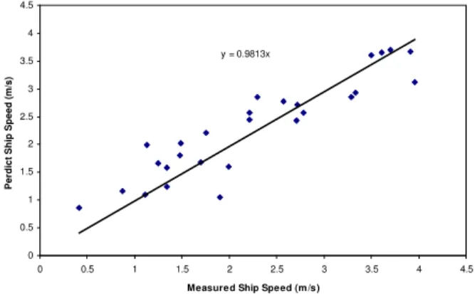
Figure 10. Yaw moment in turning circle predicted by OSIS and Polaris, Mackinaw in ice (Turning radius = 156 m, thickness = 0.625 m, strength = 650 kPa, and friction = 0.05) The full-scale trials for the R Class (Spencer, 2001) were conducted in various conditions. The data set selected for validation is from one of the trials. Figure 11 shows a comparison of the power consumption predicted by OSIS and the corresponding measurement. Despite
considerable scattering, the OSIS speed prediction agreed well with the measurement with 2% under-prediction on average (see Figure 12).
Power vs (VT) y = 2.2264x + 1569.1 y = 2.0005x + 1555.2 0 2000 4000 6000 8000 10000 12000 0 500 1000 1500 2000 2500 3000 3500 4000 4500 VT (kNm/s) P o w e r (k w ) Measurem ent OSIS750 Linear (Measurement) Linear (OSIS750)
Figure 11. Power consumption prediction by OSIS vs. measurement (power vs. VT)
y = 0.9813x 0 0.5 1 1.5 2 2.5 3 3.5 4 4.5 0 0.5 1 1.5 2 2.5 3 3.5 4 4.5
Measured Ship Speed (m /s)
P e rd ic t S h ip S p e e d ( m /s )
CONCLUSIONS
This paper presents the theoretical basis and its implementation in the OSIS-IHI software. The preliminary validation has demonstrated the accuracy of this software in simulating ship manoeuvring motions in ice using full-scale and model test data.
With the current interest in modeling and simulation of ship manoeuvring with azimuthing podded propulsion systems and local ice pressure on ship hulls, OSIS is being upgraded to extend its modelling capability in these areas.
OSIS-IHI also provides a framework for modeling the behaviour of a floating ship in water and in ice. For example, it can be upgraded with a Dynamic Positioning control module and a
Mooring System module to simulate the operations of moored ships operating with a DP system. Simple wind, wave and current modules can also be integrated into OSIS-IHI to simulate the necessary environmental conditions for such modeling.
AKNOWLEDGEMENTS
The work was performed by the Institute for Ocean Technology (NRC-IOT), with partial financial support by the Natural Science and Engineering Research Council (NSERC) and the Atlantic Innovation Fund through the Modeling and Simulation of Harsh Environments Project administrated by the Memorial University of Newfoundland Centre for Marine Simulations. Their financial support is gratefully acknowledged.
REFERENCES
Lau, M., 2006. Discrete Element Modeling of Ship Maneuvering in Ice. Proc. of the 18th
International Symposium on Ice, IAHR Ice Symposium 2006, Sapporo, Japan, Vol. 2, pp. 25- 32. Lau, M., and Derradji-Aouat, A., 2004. Preliminary Modeling of Ship Maneuvering in Ice. 25th Symposium on Naval Hydrodynamics, 8-13 August, St. John's, NL v. 2: p. 34-42.
Liu, J., Lau, M., and F. M. Williams, 2006. Mathematical Modeling of Ice-Hull Interaction for Ship Maneuvering in Ice Simulations. 7th International Conference and Exhibition on
Performance of Ships and Structures in Ice, 16-19 July, Banff, Alberta, Paper 126. Inouse, J. et al., 1981. A Practical Calculation Method of Ship Maneuvering Motion. International Shipbuilding Progress, vol. 28.
Holtrop, J, 1984. A Statistical Re-Analysis of Resistance and Propulsion Data. International Shipbuilding Progress, vol. 31.
Lau, M. and Ni, S.Y., 2009. Ship Manoeuvring in Ice Simulation Software OSIS-IHI, IOT report LM-2009-02, Institute for Ocean Technology, National Research Council of Canada, St. John’s, Newfoundland.