Bayesian population inference for effective connectivity

Bayesian Population Inference

for Effective Connectivity

by

Eric Richard Cosman, Jr.

B.S., Massachusetts Institute of Technology (1999)

M.Eng., Massachusetts Institute of Technology (2000)

Submitted to the Department of Electrical Engineering and Computer

Science

in partial fulfillment of the requirements for the degree of

Doctor of Philosophy in Electrical Engineering and Computer Science

at the

MASSACHUSETTS INSTITUTE OF

August 2005

TECHNOLOGY

(© Massachusetts Institute of Technology 2005. All rights reserved.

Author ..

Department of Electrical Engineering and C

Science

-u-,

25

Certified by ...

William M. Wells, III

Associate Professor of Radiology, Harvard Medical School

Aa_ Thesis Supervisor

Certified

by

...

...

_

W. Eric L. Grimson

Bernac-Gdj

Profesor-,of Medical Engineering

T,1fris Supervisor

Accepted

by...

Arthur C. Smith

Chairman, Department Committee on Graduate Students

ARCHIVES MASSACHUSETTS INSTRiTE OF TECHNOLOGY MAR 2 8 2006

Zj~~.

ARIES

-LIBR

Bayesian Population Inference

for Effective Connectivity

by

Eric Richard Cosman, Jr.

Submitted to the Department of Electrical Engineering and Computer Science on August 31, 2005, in partial fulfillment of the

requirements for the degree of

Doctor of Philosophy in Electrical Engineering and Computer Science

Abstract

A hierarchical model based on the Multivariate Autoregessive (MAR) process is pro-posed to jointly model functional neuroimaging time series collected from multiple subjects, and to characterize the distribution of MAR coefficients across the popula-tion from which those subjects were drawn. Thus, model-based inference about the interaction between brain regions, termed effective connectivity, may be generalized beyond those subjects studied. The posterior density of population- and subject-level connectivity parameters is estimated in a Variational Bayesian (VB) framework, and structural model parameters are chosen by the corresponding evidence criterion. The significance of resulting connectivity statistics are evaluated by permutation-based approximations to the null distribution. The method is demonstrated on simulated data and on actual multi-subject functional time series from electroencephalography

(EEG) and functional magnetic resonance imaging (fMRI). Thesis Supervisor: William M. Wells, III

Title: Associate Professor of Radiology, Harvard Medical School Thesis Supervisor: W. Eric L. Grimson

Title: Bernard Gordon Professor of Medical Engineering Readers: Polina Golland, John W. Fisher III, Hal S. Stern

Acknowledgments

I must express foremost gratitude to Sandy Wells who has been my close collabora-tor, advisor and friend for the duration of my time in graduate school. I consider myself lucky to have had a thesis advisor who was accessible enough to allow for constant interaction, and who, at the same time, allowed a great degree of latitude for independent thought. Sandy is ever supportive intellectually and practically, ac-tively engaged in technical issues, and diligent in establishing collaborations with the neuroscientists to test theoretical methods.

I am also especially indebted to Eric Grimson who has also guided me through graduate school from the outset. My positive experience in graduate school would have been profoundly different without his clarifying direction.

I would also like to thank the other members of my thesis committee, Polina Golland, John Fisher and Hal Stern, for their help in the preparation of this document. Having so many intelligent eyes inspecting my work very much improved its quality. Even from as far away as Irvine, California, Hal Stern's comments about my thesis proposal pointed new directions for investigation that had a material impact on the final content of my work.

As one who is developing methods for analysis of neuroimaging data, I have been reliant on the neuroscientific practitioners who painstakingly collect it. It was a pleasure to work with Ralph Suarez and Alex Golby of the Brigham and Women's Hospital, who provided some of the fMRI data I analyzed for this thesis. I would also like to thank others who provided functional data and unique insights about it, including Reisa Sperling, Pisti Morocz, Mark Vangel, Fa-Hsuan Lin, and Yulia

Golland.

Lastly, but not at all perfunctorily, I want to thank my friends and family for their personal support. It was a truly unique pleasure to have had all members of my family-- Morm, Dad, Christina, Niels, and Sonia- living within a twenty minute radius of school. Their advice and love has been invaluable to me. I am also grateful for my good friends Amos Benninga, Erik Snowberg, and many others, who helped

me to maintain a life outside lab. And, for the very substantial amount of time that I did spend in lab, I feel very lucky to have been working alongside such great officemates and friends as Lilla Z611ei and Florent Segonne. Their presence made the everyday experience of getting a doctorate a lot of fun.

Contents

1 Introduction

1.1 Methods of Functional Neuroimaging ...

1.1.1 Functional Magnetic Resonance Imaging (fMRI) 1.1.2 Positron Emission Tomography (PET) ...

1.1.3 Electroencephalography (EEG) . . . . 1.1.4 Magnetoencephalography (MEG) ... 1.2 Activity Detection ... 1.3 Connectivity Inference ... 1.3.1 Functional Connectivity ... 1.3.2 Effective Connectivity ... 1.4 Contributions. ...

1.4.1 A Preview of RFX-MAR Analysis ... 1.5 Thesis Overview ...

2 Technical Background

2.1 The Multivariate Autoregressive Process . . 2.1.1 Definitions ...

2.1.2 MAR(1) Representation ... 2.1.3 Stability, Stationarity and Spectrum 2.1.4 Likelihood Function ...

2.1.5 Generalizations ...

2.1.6 Maximum Likelihood Estimation . .

2.2 Random-Effects Population Inference ....

15 . . 16 . . 16 . . 17 . . 18 . . 19 . . 19 . . 20 . . 21 . . 22 . . 25 .. 27

*

2.2.1 Fixed and Independent Effects Analysis . . 2.3 The Variational Bayesian Framework ...

2.3.1 Variational Posterior Approximation . . .

2.3.2 The Expectation Maximization Algorithm

2.3.3 Variational Model Comparison ... 2.4 Summary ...

3 Multi-subject MAR Modeling

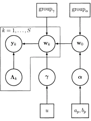
3.1 The RFX-MAR Model ...

3.1.1 Subject-separable MAR Models .. 3.1.2 Structured Inter-subject Variability .

3.1.3 A Structured Prior for the Population 3.1.4 Noninformative Precision Priors . . .

3.1.5 Exogenous Fixed Effects ... 3.2 The FFX-MAR Model ... 3.3 The IFX-MAR Model ... 3.4 Discussion ...

3.4.1 Limitations ...

3.4.2 Interpretation ...

4 Variational Population Inference

4.1 RFX-MAR Estimation ... 4.1.1 Hybrid Optimization ... 4.1.2 Update for q(w) ... 4.1.3 Update for q(A) ... 4.1.4 Update for q(-y) ... 4.1.5 Update for q(cx) ... 4.1.6 Formula for F ... 4.2 FFX-MAR Estimation ... 4.3 IFX-MAR Estimation ... 4.4 Model Selection ... . .o . . . . Coefficients . 47 49 50 52 54 57 59 59 61 62 63 65 67 68 69 . . . .72 . . . 72 . . . 73 75 . . . 76 . . . 78 . . . 80 . . . 83 . . . 85 . . . 86 . . . 87 . . . 91 . . . 93 . . . 95

4.5 Effective Connectivity Inference 4.5.1 Connectivity Statistics 4.5.2 Permutation Significance 4.6 Summary ... 5 Experimental Results 5.1 Artificial Data ... 5.1.1 One Population .... 5.1.2 Two Populations ... 5.1.3 Independent Subjects . .

5.1.4 Guidelines for Sample Siz

5.2 EEG Data ... 5.2.1 Data Description .... 5.2.2 Connectivity Analysis 5.2.3 Reproducibility ... 5.2.4 Inter-subject Regularizati 5.2.5 Discussion ... 5.3 Language fMRI ... 5.3.1 Data Description .... 5.3.2 Connectivity Analysis . 5.3.3 Discussion ... 5.4 Summary ... . . .. .. . . . e . . . .. . . . . . .. . . . .. . . . . .. . . . . .. . . . . . .. Oi . . . . . . . ... 6 Conclusion 6.1 Future Work ...

6.1.1 Open Questions for Effective Connectivity Analysis ... 6.1.2 Population Inference for Other Models ...

A Relevant Densities

A.1 The Gaussian Density ...

A.1.1 The Fisher Information Matrix ... ...

97 97 100 102 103 103 104 114 117 118 119 120 120 124 125 128 129 129 131 135 140 141 142 142 143 145 145 146

A.2 The Gamma Density ...

A.2.1 The Gamma and Digamma Functions. A.3 The Incomplete Gamma Density ...

A.4 The Wishart Density ...

B Matrix Identities and Notation

B.1 Dot Notation ... B.2 The vec Operator ...

B.3 Kronecker Product ® ... B.4 Matrix Identities ... B.5 Matrix Differentials ... B.6 Partitioned Determinants .. 151 ... . . . 151 ... . . . 151 ... . . . 152 ... . . . 152 ... . . . 153 ... . . . 153 147 148 148 149

...

...

...

...

List of Figures

1-1 Effective Connectivity Graph ... 23

1-2 EEG electrode positions and time series ... 27

1-3 EEG Ccoefficient Posterior ... ... . 31

3-1 The RFX-MAR Model ... 61

3-2 The FFX-MAR Model ... 69

3-3 The IFX-MAR Model ... 71

4-1 Pseudocode for the VB estimation of the RFX-MAR model ... . 77

4-2 Pseudocode for the VB estimation of the FFX-MAR model . ... 92

4-3 Pseudocode for the VB estimation of the IFX-MAR model ... 94

5-1 True connectivity for an artificial dataset ... 105

5-2 Population coefficient estimates ... . 107

5-3 Average coefficient estimation error ... ... . 108

5-4 Error rate of connectivity detection ... ... . 108

5-5 Variation in coefficient estimates across model structures ... . . 109

5-6 FFX-MAR vs. RFX-MAR population coefficient estimation error . . 109

5-7 FFX-MAR vs. RFX-MAR subject coefficient estimation error . . . . 110

5-8 IFX-MAR vs. RFX-MAR subject coefficient estimation error . . . 110

5-9 Inter-subject variability estimation ... ... 1... 1

5-10 Intra-subject variability estimation . . . .111

5-11 M odel order selection . . . 112

Meta-model selection ...

Two population connectivity ground-truth ...

IFX-MAR vs. RFX-MAR subject coefficient estimation error . MAP two-population RFX structuring ...

Evidence for joint vs. separate population modeling ... Detection of population differences ...

IFX-MAR vs. RFX-MAR subject coefficient estimation error . Meta-model selection for artificial independent subjects .... The RFX-MAR MAP model order p for independent subjects. 5-22 EEG electrode positions and time series

EEG Model Selection ...

EEG RFX Variability Structuring ... EEG Coefficient Posterior ...

EEG permutation null distribution ...

EEG coefficients for different subjects ... EEG reproducibility of connectivity statistics Reproducibility of EEG population connectivity EEG coefficients for a single subject ...

fMRI time series ... fMRI meta-model selection ...

fMRI RFX-MAR model-structure evidence . . . fMRI left hemisphere RFX & ARD groups . . . fMRI right hemisphere RFX & ARD groups . . fMRI coefficient posterior ...

fMRI permutation null distribution ...

fMRI connectivity graphs ... fMRI IFX-MAR connectivity ...

... . . . 121 . . . graph

...

.122

...

.123

...

.124

...

.126

...

.127

...

.127

...

.130

...

.132

...

.133

...

.133

...

.134

...

.135

...

.135

List of Tables

5.1 EEG population-level connectivity statistics ... 125

5.2 EEG reproducibility of population coefficient posterior ... . 126

Chapter 1

Introduction

Our modern view of the functional organization of the brain is based on the princi-ples of localization and connectionism: that complex cognitive function emerges from the interaction of anatomically distinct regions, each specialized to a sub-function [95, 85]. The details of this functional organization have been explored over the last few decades through a variety of methods that enable spatiotemporal measurements of brain activity under different experimental conditions [58, 48]. Historically, analysis of these functional neuro-monitoring data has focused on inference about the spatial distribution and timing of brain activity, such as in estimating the position and wave-form of an intracranial dipole based on magnetoencephalography, or in producing activation maps using functional magnetic resonance imaging. More recently, atten-tion has been drawn toward inference about the interacatten-tion among gross brain regions by viewing neural time series as the realization of a distributed random process.

In this introduction, we will discuss methods by which brain activity may be monitored, and methods which use these data to characterize the location, timing and connectivity of systems-level neural networks active during the performance of behavioral or cognitive tasks. We will also summarize the contributions of our research in the area of connectivity analysis based on functional neuroimaging data.

1.1 Methods of Functional Neuroimaging

The various methods for measuring neural activity in distributed regions of the brain differ in their spatial and temporal resolutions, and in the means by which this activ-ity is measured. Generally speaking, these methods fall into two classes: (1) those by which neural activity is observed through related physiological changes (e.g. hemo-dynamic and metabolic variations) and is sampled volumetrically or tomographically (slice-wise) with low temporal resolution; and (2) those by which activity is observed through electric or magnetic variations which are sampled sparsely in space, but finely in time. In the former class are Functional Magnetic Resonance Imaging (fMRI) and

Positron Emission Tomography (PET). In the latter class are Electroencephalogra-phy (EEG), MagnetoencephalograElectroencephalogra-phy (MEG), and intracranial electrical recording by

means of surface or depth electrodes. The different characteristics of these meth-ods have important bearing on the feasibility of activity detection and connectivity inference, so we summarize them here.

1.1.1 Functional Magnetic Resonance Imaging (fMRI)

Functional Magnetic Resonance Imaging (fMRI) assesses brain activity by monitoring

changes in blood flow and oxygenation which are referred to as the Blood Oxygen Level

Dependent (BOLD) effect [62, 92, 3]. These data may be collected tomographically

or volumetrically over time. A recent summary text of the subject [58] reports the typical in-plane linear resolution is 4 to 5 millimeters for full-brain fMRI acquisitions, and 1 to 2 millimeters for region-specific acquisitions. It also reports that 1 to 2 second temporal resolution is typical and sufficient to characterize hemodynamic variations, but that sample rates from 500 ms to 4 seconds may be useful in some contexts. Though finer temporal resolution is possible, this compromises signal strength (due to the shorter flip-angle required to reach steady-state more quickly) and/or the anatomical volume that can be scanned.

It is hypothesized that the BOLD effect is linked to changes in neural activity via the Balloon Model [13, 76, 29] which has a delayed smoothing effect in time. A

number of studies have also characterized the approximate linearity of the BOLD response to neural activity [8, 19, 100] as well as evidence of nonlinearities that may be due to saturation, habituation or other effects. Based on studies in the sensori-motor and visual cortices where neural stimulation can be quite direct, it is generally reported that the BOLD impulse response to neural activity exhibits a delayed onset of approximately 2 seconds, rises to some peak value, and returns to baseline over a total of 10 to 15 seconds [19, 100, 9, 58]. An initial and refractory dip are predicted by the Balloon Model and have been shown empirically [13, 29], but these effects are far more subtle than the primary peak. A number of studies have reported a time-to-peak interval of 4-6 seconds for visual and other BOLD impulse responses

[19, 101, 58].

Experimental protocols for fIRI experiments fall generally into three classes.

Block designs [33] refer to protocols in which experimental conditions are held constant

for an extended period of time or block. Variation between blocks may occur in a cyclic manner, such as switching back and forth between "active" and "rest" conditions so that activity under these conditions may be contrasted. Event-related designs [17] refer to protocols in which stimuli or tasks are presented or performed in a transitory manner. These cognitive or behavioral "events" may be of single or multiple types, and presented in a temporal sequence with regular or randomized spacing. Finally, a protocol may also be unstructured, for instance acquired solely while the subject is

"at rest".

1.1.2 Positron Emission Tomography (PET)

Positron Emission Tomography (PET) assesses brain activity by means of positron

emissions that are coupled to brain metabolism or blood flow by means of radioactively-tagged molecules administered intravenously [11]. Pairs of photons released by positron-electron annihilations are used to reconstruct tomographic or volumetric [2] scans of brain metabolism with spatial resolution on the order of 4mm. This spatial resolu-tion is inherently limited by the distance separating the events of positron emission and annihilation. This distance varies with isotope species, but PET resolution has

been theoretically limited to 2-3mm in general [67]. Typical temporal resolution is on the order of tens of seconds depending the time required for adequate photon counts

[109].

1.1.3 Electroencephalography (EEG)

Electroencephalography (EEG) is the measurement of electrical potential over time

by electrodes placed on the scalp. These potentials are the manifestation of the in-tegrated synaptic potentials from large populations of neurons. Event-related Brain

Potentials (ERP) refer to EEG recordings of potentials induced by an internal or

external event, such as a task or stimulus [48]. Intracranial EEG (iEEG) or

Electro-corticography (ECoG) refers to the placement of electrodes subdurally [86]. A detailed

coverage of the subject can be found in the text [90] from which information in this section is largely derived.

EEG time series are sampled with temporal resolution on the order of a few milliseconds to capture rapid electrical variations in the brain. Sites for recording have been standardized by reference to anatomical landmarks. The International

10-20 system designates 21 recording sites. The American EEG Society extended

this system to include a total of 75 locations and labels as shown in Figure 5-22 of Chapter 5. In order to sensitize the recording to different phenomena, potentials may be measured in a monopolar manner relative to a reference electrode (such as one placed on the ear), or in a bipolar manner by differencing signals from adjacent

electrodes in either the anterior-posterior or the left-right direction.

Limitations of EEG include the fact that it cannot detect activity which pro-duces "closed" electric fields, and the fact that direct inference about the location and strength of brain activity is not possible based on signals recorded at the scalp [48]. Research on intracranial source localization based on scalp EEG measurements is currently of interest. Approaches to this "inverse problem" include dipole and distributed source models which may be estimated using head models derived from anatomical MRI, or using PET/fMRI activation maps as a constraint source locations (see Chapters 7, 9 and 15 of [48] for a review).

1.1.4 Magnetoencephalography (MEG)

Magnetoencephalography (MEG) [14] refers to the measurement of magnetic fields

over time by means of SQUID magnetometers situated outside the skull. These fields arise from synchronized activity of neuronal populations and can be sampled with millisecond temporal resolution. Modern whole-head MEG scanners may contain hundreds of measurement channels. A variety of gradiometric coil configurations can be employed to adjust the sensitivity of MEG measurements. For instance, second-order axial gradiometers can improve the spatial locality of measurements by canceling magnetic fields from distant sources. The article [45] contains an excellent review of MEG technology and physiology and was the primary source for this section.

MEG is closely related to EEG and provides complementary electromagnetic infor-mation. Source localization with MEG can be performed with higher spatial accuracy since electric fields may be strongly affected by tissue inhomogeneities in the head, whereas magnetic fields are primarily influenced by currents in the brain. Approaches to the "inverse problem" of source localization based on MEG recordings are similar to those for EEG. The Equivalent Current Dipole (ECD) approach involves estima-tion of the locaestima-tion, amplitude and orientaestima-tion of one or more dipole sources which could explain the observed MEG signal [102]. Current-distribution approaches, such as Minimum-norm Estimates (MNE) [46], model MEG signals as originating from distributed sources, whose location may be informed by structural MRI and/or fMRI activation data under similar experimental conditions [68, 18].

1.2 Activity Detection

Much of the efbfort in the analysis of functional time series has been directed at

lo-calizing and characterizing the temporal structure of brain activity related to the

ex-perimental conditions under which data was collected. Source localization techniques for EEG and MEG are examples of this kind of analysis, whereby the locations and waveforms of brain activity that produced extracranial measurements are estimated over time. The waveform of raw EEG/MEG time series is also of interest but may be

corrupted by high levels of noise. This noise can be reduced, for instance, by averag-ing over repeated ERP trials. Methods of topographic analysis by which current or energy density estimates are interpolated between EEG electrodes [104, 110, 91] have been proposed and applied in a variety of ERP experiments [55, 116] to characterize the spatial distribution of electrical patterns over the scalp over time.

Localization of brain activity in fMRI and PET is performed essentially by as-sessing correlation between observations at each voxel and the experimental protocol, whose conditions vary over the functional acquisition. Many variations on this

pro-cess of protocol-dependent activity detection have been developed. For fMRI, these include modeling the BOLD response with varying degrees of elaboration [114, 17, 51, 29], accounting for local spatial correlation between voxels [12, 22, 96], and temporal noise modeling [98]. Other work has focused on the design of experimental protocols for the purpose of optimizing detection power [16, 38].

Considerable work has also been directed toward population/group analysis so that inference about the location of protocol-related neural activity may be general-ized to the greater population from which studied subjects were drawn. In the area of fMRI analysis, linear-Gaussian hierarchical models (see Section 2.2 on random effects (RFX) analysis) have been used extensively for this purpose. Early work used a sum-mary statistic approach [57], whereas application of the EM algorithm enabled more general models to be considered [34, 31]. A sampling approach is developed in [113]. Non-parametric population inference for fMRI activation detection is developed in

[56, 89] to relax the assumption of Gaussian uncertainty that characterizes typical RFX analysis.

1.3 Connectivity Inference

The techniques referenced in the previous section are unified in that they approach the problem of activity modeling in a local manner, that is, by treating distinct anatomical regions individually. This is consistent with the principle of localization in brain organization, but it avoids the principle of connectionism, which posits that

complex cognitive function arises from the interaction among distinct brain regions. Since functional time series are a manifestation of this joint operation, it is natural to try to infer that interaction based on these data.

Two classes of methods have been proposed for joint analysis of functional time series collected from different brain regions. The first, which is sometimes termed

Functional Connectivity analysis, includes exploratory methods aimed at the

identifi-cation of similar patterns of activity across regions of interest, without modeling the mechanisms by which these patterns arise [6]. The second, which is termed Effective

Connectivity [49] or Granger Causality [60, 71] analysis, includes methods by which

functional time series are modeled explicitly as the realization of a dynamical system in which local activity may affect activity in anatomically distinct regions.

1.3.1 Functional Connectivity

Techniques for functional connectivity analysis have been applied to PET, fMRI, EEG and MEG time series. The texts [37, 23, 20] review some of these techniques. They include the assessment of correlation [40, 47] and phase-locking [20], time series clustering [43], and various spatiotemporal decompositions which are specializations of principle components analysis (PCA) [35], singular value decomposition (SVD) [30, 80] and independent components analysis (ICA) [75, 82]. These last methods are also used to decompose functional time series in an exploratory manner, for instance to distinguish components related to the experimental protocol, physiological processes, and other noise.

The literature contains examples of studies in which functional connectivity anal-yses have produced sensible results using fMRI (e.g. in showing correlation between language areas [47], or in resting-state motor regions [6]). But, caution should be urged in interpreting these results as a demonstration of functionally-significant con-nectivity among brain regions. These methods essentially group signals on the basis of correlation or other measures of similarity, which could arise due to a direct interac-tion between or among regions, or due to the common influence of an exogenous factor such as the experimental protocol or non-functional physiological processes.

Further-more, since clustering by these methods implies a symmetric relationship between regions, directional network descriptions such as causal influences or information flow cannot be inferred.

1.3.2

Effective Connectivity

Effective connectivity is defined as the influence that one brain region exerts on an-other under a given interaction model [49]. Analysis of effective connectivity differs from that of functional connectivity in that it is based on estimation of a generative model of neurological time series. In particular, functional measurements made in specified brain regions are modeled as the realization of a distributed random process in which local changes may affect other regions, possibly reciprocally.

Effective connectivity analysis is motivated by the possibility of using informa-tion contained in funcinforma-tional time series collected simultaneously from multiple brain regions to address hypotheses about the interaction of these regions under particu-lar experimental conditions or due to some neurological disorder. Such hypotheses may be about the presence or temporal structure of an influence between brain re-gions, about whether that influence is conducted through an intermediary region, or about whether that influence is modulated by activity in another region or by some experimental condition.

Figure 1-1 shows a hypothetical effective connectivity analysis on a sensorimotor network based on MNE MEG time series. The graph indicates evidence from these time series that the interaction between the primary sensory cortex in the left hemi-sphere (L SI) and the primary motor cortex in the right (R MI) is mediated by the secondary sensory cortex in the left hemisphere (L SII), under the conditions of a particular experimental protocol.

Directional inference of this kind is enabled by explicitly modeling the way func-tional time series were produced, and incorporating into that model a parameter-ization of inter-regional influences. Numerous models have been proposed for this purpose to capture different phenomena present in functional time series. Notable examples include the following:

Figure 1-1: The effective connectivity inferred for a hypothetical sensorimotor network based on MEG-based dipole models. L SI = left primary sensory cortex, L SII = left secondary sensory cortex, R MI = right primary motor cortex, R SII = right secondary sensory cortex

* Structural Equation Modeling (SEM) [81] involves constrained modeling of the covariance of multivariate measurements in a time-invariant manner. Di-rectional influence in a network can be inferred by constraining some diDi-rectional influences to be zero on the basis of prior functional/anatomical knowledge. SEM has been used to analyze network interactions based on fMRI, EEG and MEG [81, 66].

* Volterra kernels [39] can describe a causal relationship between a system output and the recent past of an input by means of higher-order convolutions. They have been used to characterize non-linear (i.e. asynchronous) coupling be-tween pairs of functional time series collected by MEG. A limitation of pairwise modeling is that it may not be able to distinguish direct interactions between regions from those that are indirect and conducted through other observed brain regions.

* Multivariate Autoregressive Modeling (MAR) [71] falls in the class of "black-box" or regression approaches to system identification [70], and charac-terizes observed multivariate time series as a time-invariant linear regression of their recent past. This is described in detail in Section 2.1. It has been applied to modeling network interactions based on EEG, MEG, fMRI and intracranial

electrical monitoring [93, 60, 50].

* Dynamic Causal Modeling (DCM) [32] refers to a state-space model [70] specific to fMRI. Neural dynamics are described by a multivariate ARX(1) model which includes bilinear terms such that observed exogenous variables (e.g. experimental conditions) can modulate the interaction between brain regions. These dynamics are modeled as observed through the Balloon model for the BOLD response, whose parameters are estimated for each region of interest separately.

Volterra kernels, MAR and DCM characterize effective connectivity by model-ing particular brain regions as variables in a causal, dynamical system (cf. SEM). Interregional influence is inferred via parameters that govern the prediction of one variable/region on another under these models, so our interpretation of results such as those shown in Figure 1-1 should be interpreted accordingly. In particular, evidence of a predictive relationship between modeled regions of interest does not alone imply a causal relationship. Indeed, a predictive relationship between two variables may be observed even if a direct causal relationship is absent. For instance, two regions may both be subject to some unmodeled influence so that one region is predictive of the other, even if there is no direct interaction between them.

Connectivity analysis of this kind is closely related to the concept of Granger

Causality due to Wiener [112] and Granger [44], by which casual inference is

consid-ered from a statistical viewpoint. Specifically, it is said that one variable "Granger causes" another, if past observations of one variable reduce the prediction error of another.

It should be emphasized that these models represent gross simplifications of actual neural dynamics. They are proposed to utilize what connectivity information may be available through current neuroimaging methods and are not universally applicable. It would be theoretically useful to be able to estimate a model that is representative of actual brain function, for instance, being time-varying, involving both local and interregional neuronal dynamics, combinations of inhibitory and excitatory

interac-tions, global modulatory effects, and so forth. However, this is implausible given the present temporal and spatial resolution of methods of functional and anatomi-cal neuroimaging. The limitations of current connectivity models, while necessary, warrant care in their application and in the neuroscientific interpretation of results they produce. Caveats are similar to those mentioned in our overview of functional connectivity, and sources of bias include the potential incompleteness of the system description; the effect of non-functional noise processes (e.g. those due to physiologi-cal processing, acquisition-related artifacts, and data processing); and assumptions of linearity, stationarity and Gaussianity, among others. These biases may both obscure evidence of true inter-regional interactions, and create the appearance of erroneous ones. Nevertheless, promising results have been shown for these methods in the litera-ture [32, 60, 50, 83], and detailed analysis of the strengths and limitations of different connectivity models for different imaging modalities is an area of active research [63].

1.4 Contributions

It is of neuroscientific interest to determine which interactions between modeled brain regions are characteristic under experimental conditions, within the population from which studied subjects are drawn. Population, or group, inference of this kind has been a central topic in the localization of protocol-related brain activity based on functional time series [57, 34, 31, 113]. However, to our knowledge, models for effec-tive connectivity have been applied only in subject-independent manner. As such, statistical inference about connectivity is limited to the specific subjects included in a study. The primary aim of this thesis is the exploration of population inference about effective connectivity.

We propose a generative, or Random effects (RFX), approach to modeling multi-subject functional time series, such that the effective connectivity parameters of all subjects are estimated jointly along with a density describing the variation in those parameters across the population from which studied subjects were drawn. This en-tails the use of a strong model of inter-subject variation that enables single-population

characterization and adaptive regularization across subjects. While such joint esti-mation of connectivity under SEM, MAR, DCM or other models could be valuable for neuroimaging studies, we have chosen the MAR process as a starting point for our investigations. We made this selection primarily because of the generality of the MAR process and its demonstrated applicability to different neuroimaging modalities

[60, 93, 50].

In this work, we develop the RFX-MAR model which parameterizes the interac-tions of specified brain regions for each subject using the MAR process, and describes the variability in those subject-level models by the mean and variance of their MAR coefficients. We estimate its population- and subject-specific parameters in a Varia-tional Bayesian (VB) framework, and characterize effective connectivity at the pop-ulation level by inference on the posterior of the MAR coefficients' means, which we refer to as the population-level MAR coefficients. Specifically, we compute statistics related to evidence of non-zero directional influence between each pair of monitored brain regions under the MAR model, across the sampled population. Structural pa-rameters of the RFX-MAR model are selected by an approximate maximum evidence criterion.

In summary, the contributions of this thesis include:

* Motivation of the problem of population/group inference about effective con-nectivity.

* Development of a random effects model for MAR-based effective connectivity.

* Development of a variational Bayesian framework for estimation and inference under the proposed models.

* Analysis of inter-subject and variability in effective connectivity based on func-tion time series collected by means of EEG and fMRI.

A Vertex F5 F6 T7 T8 P3 P4 pN\~mVVlfrAA/C 250 500 750 1000 Time (msec)

Figure 1-2: (Left) Standard EEG electrode positions and labels as designated by the American EEG Society (Image Copyright 1990 American Electroencephalographic Society). (Right) EEG time series from six of these channels in one subject.

1.4.1

A Preview of RFX-MAR Analysis

To provide context for this thesis, we preview its proposed analytic methods by exam-ple. Specifically, we summarize methods of modeling and inference for EEG recordings at 64 standard electrode locations (Figure 1-2) on the scalps of 20 subjects during a picture-matching task. These data and their analysis is described in detail in Section 5.2. To facilitate this streamlined discussion, some of the notation used in this section differs slightly from that used in the remainder of the document.

Data Preparation

Functional time series are collected under experimental conditions intended to evoke activity in specific brain systems. The brain regions of these systems may be selected for connectivity analysis either on the basis of the experimenter's prior knowledge, or by activity-localization methods. Since the number of parameters for an uncon-strained connectivity model varies as the square of the number of modeled regions,

these regions must be selected to keep this number small. Otherwise, interactions may need be constrained so that model complexity conform to the amount of data available. For unconstrained connectivity analysis of the EEG data, we selected six anatomically distinct regions that showed high surface energy as indicated by the neuroscientists who collected them.

The selection of representative time series for these regions of interest (ROI) rep-resents another important modeling choice. For these analyses, we used 1 second of data from one EEG channel in each anatomical region. These are plotted for one sub-ject Figure 1-2. Alternatively, we might have averaged signals from multiple channels, or extracted multiple time series for each ROI using principle components analysis (had more channels within each ROI been available for this purpose).

MAR Connectivity Modeling

In this thesis, we use the Multivariate Autoregressive (MAR) process [71] as a model for effective connectivity. Under this model, the observed measurement of neural activity in each ROI at the present time is a linear, time-invariant function of the past observations in all ROIs. Specifically, the observed EEG measurements at time n are collected into a row vector yn and are modeled as a specialized linear regression of the p past values of these time series,

yn = v + y_lA(1) + * + Yn-pA(p) + en, n 1,...,

(1.1)

where v is an intercept, and en is temporally-white, stationary noise with Gaussian distribution K(0, A-'). The parameter p is referred to as the model order. The series of matrices A(l), I = 1, . . ., p, are referred to as the coefficient matrices and

param-eterize all causal relationships between modeled regions of interest. Specifically, the coefficients Aij(1), . . , Aij(p) parameterize the prediction of region j based on region i. When this vector is uniformly zero, Aij(l) = 0, I = 1, ... , p, there is no direct causal

relationship between these ROIs. For simplicity of reference, we sometimes collect all MAR coefficients into a single vector w _ (A(1), . . ., A(p)). Further information

about the MAR process is given in Section 2.1.

Random Effects MAR Modeling

The purpose of the Random-Effects MAR model (RFX-MAR) is to characterize ef-fective connectivity in the larger population from which subjects were drawn for the EEG study. This is accomplished by estimation of the sampling density for the stud-ied subjects. Specifically, a "population density" is estimated which characterizes the variation in subject-specific MAR coefficients, since it is these coefficients that param-eterize inter-regional connectivity under the MAR model. If the observed subjects and the assumed form of the population density are representative of a broader pop-ulation, analysis of the population density may enable generalization of connectivity

inference to that population.

Under the RFX-MAR model, the EEG time series collected from each of S - 20 subjects are modeled by a subject-specific MAR process, each with its own set of MAR coefficients wk, where k - 1,...,S indexes subjects. Each set of subject-specific MAR coefficients is assumed to be drawn independently from a Gaussian density with mean w0 and diagonal covariance r-l:

~Wk f (w J; W 0, r-1) (1.2)

The covariance has a special form such that coefficients are grouped on the basis of the degree of inter-subject variability they exhibit. This structuring of RFX variability is motivated by the fact that coefficients vary by different degrees across the population, possibly related to the fact that coefficients may have vastly different magnitude. As such, it would be inappropriate to model their inter-subject variance identically with a single parameter. On the other hand, estimation of a different variance parameter for each coefficient limits estimation power. A compromise between these extremes involves the estimation of relatively few variance parameters, each associated with a disjoint subset of all coefficients. The specific association of coefficients into RFX variability groups, and the number of groups, is a modeling choice that is formalized

as follows:

group(i) - the RFX group of

= h) (13)

vh -=

Zi1

6(group(i) = h)

r

₁

These definitions amount to the placement of inter-subject variance ah 1 on the

diag-onal of covariance matrix r-1 at the index of coefficient [Wk]_i when that index i is

associated with RFX variance group h.

The posterior of the population mean w0 is the ultimate target of population

infer-ence about MAR-based connectivity. These parameters, to which we will refer as the "population coefficients", characterize which predictive relationships are non-zero on average across the population from which studied subjects were drawn. Specifically, population inference will proceed by quantification of the posterior implausibility that the population coefficients associated with an inter-regional interaction i

j

are uniformly non-zero, i.e. A°j(1) - 0, = 1,..., p.

The RFX-MAR and other related models are developed in detail in Chapter 3.

Population Inference

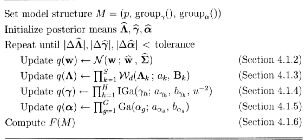
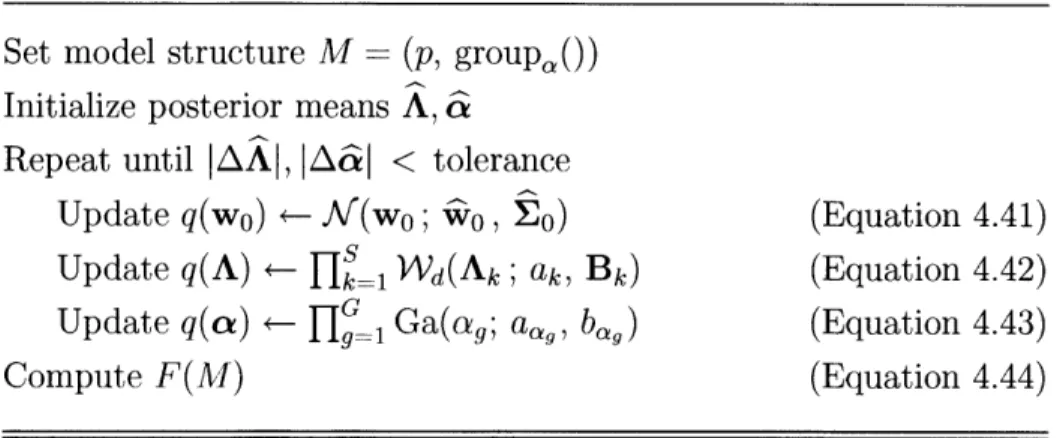
In this thesis, we propose a Bayesian framework for estimation and inference under the RFX-MAR model by specifying noninformative priors for all variance parameters. As such, inference about model parameters will proceed based on their posterior dis-tribution, which characterizes uncertainty in these parameters after having observed the data. An advantage of working in a Bayesian framework is that the likelihood (a.k.a. the "evidence") of different models of the data can be evaluated by integration over unknown parameters, and used as an objective criterion for model selection. For the RFX-MAR model, the MAR model order p and the RFX variability structuring are two modeling choices that may be selected on this basis by search over different settings.

For the proposed model, the posterior of real-valued parameters and the likelihood of different models cannot be computed in closed-form. In this work, we approximate

To: F5 To: F6 To: T7 To: T8 To: P3 To: P4 2 ~ ] 2 F 2 l I i 0 r j rýý -1 1-11 -1 1 I 1 2345 1 2345 1 23 6 2 1 0

-11

. . I

-I

l

lags lags lags lags lags lags

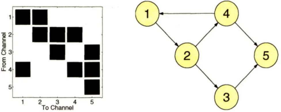
Figure 1-3: (Left) The posterior of the population-level coefficients for each inter-regional interaction plotted as marginal posterior confidence intervals, arranged in the form of a connectivity-matrix. The background of subplot (i, j) is colored black when the absence of interaction i -- j is implausible. (Right) The corresponding effective connectivity graph, in which within-channel interactions were omitted for clarity.

these quantities using the Variational Bayesian (VB) framework. The VB framework is described generally in Section 2.3, and the VB algorithm for the RFX-MAR model is developed in Chapter 4.

For the EEG data, we search over different settings of structural model parameters in a heuristic manner, and find, for example, that model order p = 5 has maximum approximate likelihood/evidence. Population inference then proceeds based on the posterior of the population coefficients wo given these maximum-likelihood structural parameters. In the VB framework, it happens that this posterior has a Gaussian form Af(W0o, (00)), with mean 0O and covariance i•(O). We can display these

suffi-cient statistics in the form of a connectivity matrix as shown in on the left side of Figure 1-3. In this representation, the posterior of population-level coefficients asso-ciated with inter-regional interaction i -- j is shown in subplot (i, j). Specifically, these coefficients are the elements of wo that are denoted A9 (1),..., A (p). For each coefficient of each interaction, a marginal posterior confidence interval is shown as a vertical bar that represents both the posterior mean and variance of that coefficient. The bar is centered at the posterior mean, and its height shows an interval that

con-L.

LL

2

-1t

1....

I

-1

1.

tains, say, 99% of the posterior probability about that mean. Therefore, a taller bar indicates greater marginal posterior uncertainty for a population coefficient. Note that each subplot in Figure 1-3 contains five posterior confidence bars. This corre-sponds to the selected MAR model order of p = 5. The marginal posterior confidence intervals are shown for the coefficients in each subplot in order of increasing lag, from left to right.

By inspection of the plotted posterior confidence intervals relative to the zero-axis, we can get a sense of whether an interaction between ROIs is plausibly non-zero a

posteriori. When all bars for a given predictive relationship i - j intersect the

zero-axis we may decide that we cannot rule out the possibility that such a relationship does not exist. One such interaction is P4--F6, whose coefficients are shown in subplot (5, 2). We can formalize this intuitive analysis by computation of a statistic based on the posterior of w0 which quantifies the posterior implausibility that its associated population coefficients are uniformly zero. In particular, the connectivity statistic for interaction i -+ j is a function of the Mahalanobis distance from the

posterior mean of its associated coefficients (A°(1),...,(p)) to the zero vector,0

,...,), Aij(P)) to the zero vector,

under the posterior distribution. Detailed development of these statistics is given in Section 4.5.1.

By thresholding these connectivity statistics, we can report the results of our con-nectivity analysis in two ways. First, we can color black the background of subplot

(i, j) in the connectivity matrix shown in Figure 1-3 when that interaction is

im-plausibly zero. Furthermore, we can draw effective connectivity graphs as shown on the right side of Figure 1-3, where displayed arrows correspond to the interactions highlighted in the connectivity matrix. For instance, the arrow from channel T7 to channel F5 indicates that T7 is predictive of F5 on average across the sampling population. The posterior of population coefficients for this interaction are shown in subplot (3,1) of the connectivity matrix representation. By close inspection of this subplot, we can find one or more posterior confidence bars which do not intersect the zero-axis. On the other hand, no arrow is shown from channel P4 to channel F5 in the connectivity graph, since the posterior mean of the coefficients for this

interac-tion was not remote enough fromn the origin (in the Mahalanobis sense) to warrant its inclusion in the connectivity graph at the selected threshold. The posterior of those coefficients is represented in subplot (5, 1).

In a Bayesian framework, the described posterior analysis is sufficient for the purpose of connectivity inference. However, since we are thresholding statistics to test for interactions between ROIs, questions inevitably arise about the specificity of this inference. To address these questions, we estimate this specificity by means of permutation approximations to the null distribution of connectivity statistics, i.e. the distribution that arises by assuming an interaction is zero at the population level. This method is detailed in Section 4.5.2.

1.5 Thesis Overview

In the next chapter, we review background material of central importance to the thesis. This includes information about the multivariate autoregressive (MAR) pro-cess, random effects (RFX) analysis, and the variational Bayesian (VB) method for posterior estimation and maximum evidence model selection.

Chapter 3 details three models we have proposed for the purpose of MAR mod-eling of multi-subject neurological time series. They are the RFX-MAR, FFX-MAR and IFX-MAR models which represent random effects, identical and subject-independent MAR modeling, respectively. We estimate these models in a Bayesian framework, so this description also includes motivation for and specification of all priors employed.

Chapter 4 discusses aspects of Bayesian inference for the multi-subject MAR mod-els defined in Chapter 3. In it, we describe a specialized version of the VB algorithm for estimation of the posterior on all real-valued model parameters. We also dis-cuss a method for selection of structural parameters in an approximate maximum evidence framework, using the VB model selection criterion. Finally, we show an approach to connectivity inference at the population and subject levels based on the estimated posterior of population- and subject-level MAR model coefficients.

Per-mutation methods are also proposed to estimate the significance of this connectivity inference.

Chapter 5 describes experiments conducted using the RFX-MAR, FFX-MAR and IFX-MAR models. We begin with a validation section which details performance of our methods based on synthetically-generated data for which the underlying model is known. We also show results of our connectivity analysis on a variety of functional time series, including:

* EEG time series collected in an event-related protocol. We use the relatively large number of subjects contained in this study to investigate the reproducibil-ity of our methods.

* fMRI time series collected during a language task from multiple subjects. We show evidence of lateralization in connectivity patterns, and provide detailed discussion pertaining the effective connectivity analysis using fMRI time series

in general.

Chapter 2

Technical Background

In this chapter we discuss technical concepts and background central to the thesis. These include the MAR process, population inference, and variational Bayesian esti-Imation.

2.1 The Multivariate Autoregressive Process

The Multivariate Autoregressive (MAR) process models the temporal dynamics of multivariate systems causally and without hidden state variables, such that multi-variate measurements at the present time are a linear function of measurements in the past. This kind of parametric process has been used to identify the linear, time-invariant (LTI) system dynamics and spectra of multichannel time-series data in a

mnumber of contexts, including economics and neuroimaging [71, (60, 93, 50]. I

neu-roimaging, the MAR process has been used to model and test effective connectivity based on neurological data collected by fMRI, EEG and direct electrical recording. Since the MAR process is strictly causal, it can model directional influence between channels, and elucidate causal chains and loops.

This section contains background information about the MAR process relevant to this thesis. For a thorough classical treatment of the MAR process, we direct the reader to the text [71]. The text [70] presents the MAR model set in the larger context of system identification. Note that the MAR process is also known by the

abbreviations VAR and MVAR.

2.1.1

Definitions

The real-valued, d-dimensional sample y E Rd of a MAR(p) process at time n is a linear combination of the past p samples, a fixed intercept v, and temporally-white,

stationary noise en c ad distributed as

F(0,

Yn

= v + Alyn-l

- +

+

2.1.2 MAR(1) Representation

Any MAR(p) process with p > 1 can be represented as a MAR(1) process by the

transformation [71, 88], Yn Yn-1 Yn-p+l E Rdp _{V =}

v

A=

[

Al

.- Ap_

1

A]

where n E Rd is sample from a MAR(p) process, n E

equivalent MAR(1) process, and Id(p-1) is the d(p- 1) x

This transformation allows us to apply the properties of MAR process of arbitrary order.

Rdp is a sample from the

d(p- 1) identity matrix.

the MAR(1) process to a

A4-

Ed-Lo 0

-2.1.3 Stability, Stationarity and Spectrum

This section is adapted, in part, from the text [71]. By recursive substitution using Equation 2.11, and denoting the multiplication of i copies of A1 as A', a MAR(1)

process can be written in moving-average (MA) form,

i j-1

yn

- (I +

E

A')v

+ Alyj +

E-

Ae

i

i=O i=O

j-o

(i

-Al)-lv +

e-i

(2.3)

i=O

if either of the following equivalent conditions holds:

(a) IAi < for all eigenvalues Ai, i = 1, . . , d of A1 (2.4)

(b) Id-A1q[ z 0 for q < 1 (2.5)

A MAR(1) process which satisfies these conditions is called stable, and has Ai - 0 as j - oo. The mean and autocovariance of a stable MAR(1) process are

Y

- {y } = (Id- Al)- (2.6)

Oy(m)

-

{(yn-

£{)(ym - -t)'}

=

E

A7+A--1Al'

(2.7)

i=O

Therefore a stable MAR(1) process is also stationary.

To investigate the effect that one variable has on another in the context of the whole system, one may inspect the impulse response of the system whose input is en, and whose output is Yn. The response evoked in variable i due to a unit change in variable j at n = 0 is the (i, j)th element of the matrix hn = Anun, where u is the discrete unit step function. This can be seen by setting e = uj6(n) in the MA representation (Equation 2.3), where uj is the jth coordinate vector in Rd (or simply

by interpreting that equation as a convolution):

00

n-H A

= (h

(2.8)

i=O

The directed transfer function H(z) is defined as the (component-wise) z-transform of the impulse response h and characterizes the spectral characteristics of the di-rected interaction between variables in a MAR(1) system [60]. By eigendecomposition of Al, the z-transform converges for zl > maxi Ai, and thus is defined on the unit circle z ej27rf precisely when the corresponding MAR(1) system is stable:

H(z) = (Id- Alz-1) -1 (2.9)

The (cross-)spectrum Sy(z) of a MAR(1) process is the z-transform of the autoco-variance function

4by(m).

Sy(z) = Z{qy(m)} - H(z)A-1H(z)' (2.10)

Autoregressive Spectral Estimation is performed by estimating the parameters of

a MAR process for a sample of a multivariate random process, and then computing its spectrum at frequency f by setting z - ej 2,f _{[61, 105].}

Using the equivalent of the MAR(1) representation for a MAR(p) process (Section 2.1.2), it is straightforward to show equivalent properties for MAR(p) process. In particular, a MAR(p) process is stable iff either of the following equivalent properties hold:

(a) AiI< 1 for all eigenvalues A, i - 1, .. , d of A (2.11)

(b) ApqPl . #id-Alq- 0 for ql < 1 (2.12)

The impulse response for a stable MAR(p) process can be written h = JAnJ' by

Y

=

J(Y" -

) =

JAlJ'en-l

-

'JAiJ'Jen1

(2.13)

i=O i=O

Similarly, its directed transfer function and spectrum are

H(z)

=

Sy(z) H(z)A-'H(z)' (2.15)

and its mean and autocovariance are

u = J(Id-Al)-'J'v

(2.16)

00

y (m) ZEhm±iA-1 h'

(2.17)

i=O

2.1.4 Likelihood Function

Though it was convenient to treat the MAR process as defined for all time, only a finite sample will be available to estimate unknown MAR parameters for real data. In this section, we present a finite-sample likelihood function for the MAR process for the purpose of such estimation. Note that we change notation slightly to write this function in standard regression form and to disambiguate indexing over time with that over subject for the purpose of multi-subject MAR modeling in Chapter 3.

We rewrite the zero-mean MAR(p) process for discrete time samples n = 1, .. , N,

~~P ~ ~ ~ ~ ~ ~~[A(1)

Yn.

=

Y(-p).

+E.

(2.18)

1=1[

I=n LA(p)

wW

A(l) E Rdxd, = 1,.. .,p, is a series of matrices comprising the coefficients of the MAR model; and En. E Rd is temporally-white, stationary noise with distribution A/(0, A-1). We replace a matrix or sequence index with a large dot to refer collec-tively to elements corresponding to all values of that index. The coefficient matrix A(l) is the transpose of Al defined in Equation 2.1, and the sequence of these matrices is combined into a single coefficient matrix W. The past p multivariate samples at time n are collected into a single row vector Xn..

Stacking these equation for every sample n = 1, . . , N, we get a matrix regression:

Y=XW+E (2.19)

We denote the p coefficients which parameterize the direct influence that channel i has on channel j as Aij(.) E RP, and refer to this as the Direct Influence Function (DIF) from channel i to j. When the purpose of MAR-based effective connectivity analysis is inference about the presence of non-zero interactions between channels, the relevant tests are of whether the DIF for each pair of channels is non-zero Aij(.) 7 0. The covariance A-1 E Rdxd characterizes an instantaneous interaction between each

pair of channels, or the common influence on pairs of channels by some exogenous influence.

Since each row of Y is independent and identically distributed (D), the likelihood function for MAR models can be written as follows.

N

p(Y

I

A(Yn.;

A-')

n=1

1 N

(2) rNd/2

AIN/

exp - 2

(Yn. -Xn.W)A(Yn.

-XnW)}

(2.20)

n=l

(2,r) J/2A / exp

{-

use its vectorized form,

p(y I w,A) A(y; (Id X)w, A-1 ® IN) (2.21)

where we define y vec(Y) E RNd, w vec(W) E RM. We accomplished this by

vectorizing Equation 2.19 using the identity in Equation B. 11, and by computing the covariance of vec(E) as follows, where (Z)ij denotes the (i, j)th jNXN block of an

arbitrary matrix Z:

(cov(vec(E)))i j - {E.iE'.j} [A-1]ijIN E NxN (2.22)

(2.22)

cov(vec(E)) -= A-1 IN

2.1.5 Generalizations

Neuroimaging experiments are commonly associated with time-varying stimuli or tasks. Or, it may be known that recorded time-series are influenced by a noise process which is not temporally white. For example, low-frequency baseline shifts are common in fMRI data. Encodings of such exogenous influences can be added as additional columns U C Rrxd in regression matrix X of Equation 2.18 without affecting analysis, except to change the number of coefficients d2_{p- + dr in W.}

X. - [Y( Y(n) -l. .. (n-p). Un.] (2.23)

These additional regressors account for bias in the noise process, and do not influence system dynamics per se, which remain time-invariant as parameterized by A(*). This kind of specialized model is referred to as a multiariate ARX model, where the "X" stands for "exogenous" [70].

It may be of interest to model nonlinear coupling between regions of interest. This can be approximated in the MAR framework by adding new variables which are nonlinear functions of data from other variables. For instance, bilinear influences can be modeled by adding a channel whose time-series is composed of the product of two other channels. Thus, the correlation between two brain regions may influence a

third, or vice-versa [50].

Lastly, it need not be the case that the regressors for each channel are identical, as presented above (Equation 2.19). For instance, some of the coefficients governing the interaction between two channels might be set to zero a priori, a higher model order might be required for some interactions, or different exogenous influences may be specified for different channels. If this is the case, Equation 2.21 takes a slightly different form, in which Xi contains the regressors for channel i:

p(y

J(y;

A

0

2.1.6 Maximum Likelihood Estimation

In this section, we derive the ML estimates for the parameters of the MAR pro-cess, whose likelihood is given in Equation 2.20. While the ML framework often has been used for MAR estimation [60], its utility is limited by the large amount of data required to fit these (d2) parameters reliably. A Variational Bayesian frame-work for MAR estimation has been proposed which relieves this data requirement to some degree, by means of a prior that regularizes coefficient magnitudes, preventing overfitting [93].

The log-likelihood L of a MAR process follows directly from Equation 2.20,

Nd

N

L

---

₂

log27r

+

-log

₂₂

A -

tr (AZ'Z)

(2.25)

where we define Z Y - XW. We can write the first differential in a useful form by defining A = C'C, with C arbitrary, to constrain A to be symmetric and positive definite, and by using facts of matrix calculus in Appendices B.4 and B.5.