Are Consumers Poorly Informed about Fuel
Economy? Evidence from Two Experiments
The MIT Faculty has made this article openly available.
Please share
how this access benefits you. Your story matters.
Citation
Allcott, Hunt and Christopher Knittel. "Are Consumers Poorly
Informed about Fuel Economy? Evidence from Two Experiments."
AEJ: Economic Policy 11, 1 (February 2019): 1-37. © 2019 American
Economic Association
As Published
http://dx.doi.org/10.1257/pol.20170019
Publisher
American Economic Association
Version
Final published version
Citable link
https://hdl.handle.net/1721.1/130334
Terms of Use
Article is made available in accordance with the publisher's
policy and may be subject to US copyright law. Please refer to the
publisher's site for terms of use.
1
Are Consumers Poorly Informed about Fuel Economy?
Evidence from Two Experiments
†By Hunt Allcott and Christopher Knittel*
It is often asserted that consumers are poorly informed about and inattentive to fuel economy, causing them to buy low-fuel economy vehicles despite their own best interest. This paper presents evidence on this assertion through two experiments providing fuel economy information to new vehicle shoppers. Results show zero statistical or economic effect on average fuel economy of vehicles purchased. In the context of a simple optimal policy model, the estimates suggest that current and proposed US fuel economy standards are significantly more stringent than needed to address the classes of imperfect information and inattention addressed by our interventions. (JEL C93, D12, D83, D91, L62, Q48)
C
onsumers constantly choose products under imperfect information. Most goods people buy have many attributes, and it is difficult to pay attention to and learn about all of them. This opens the door to the possibility that people might make mis-takes: maybe they should have signed up for a better health insurance plan with a wider network and lower copays, and maybe they wouldn’t have bought that coffee if they knew how many calories it has. Indeed, there is significant evidence that consum-ers can make systematic mistakes when evaluating products, either due to imperfect information about costs and benefits or by failing to pay attention to some attributes.1These issues are particularly important in the context of buying cars. Academics and policymakers have long argued that consumers are poorly informed and cognitively constrained when evaluating fuel economy. Turrentine and Kurani’s (2007, 1213) structured interviews reveal that “when consumers buy a vehicle,
1 See, for example, Abaluck and Gruber (2011); Bollinger, Leslie, and Sorensen (2011); Barber, Odean,
and Zheng (2005); Grubb (2009); Handel and Kolstad (2015); Hossain and Morgan (2006); Jensen (2010);
Kling et al. (2012); and others.
* Allcott: Department of Economics, New York University, 19 West 4th Street, 6th floor, New York, NY 10012,
NBER, and E2e (email: hunt.allcott@nyu.edu); Knittel: Sloan School of Management and Center for Energy and
Environmental Policy Research, MIT, 100 Main Street, Cambridge, MA 02142, NBER, and E2e (email: knittel@
mit.edu). We are grateful to Will Tucker, Jamie Kimmel, and others at ideas42 for research management and to Skand Goel for research assistance. We thank Catherine Wolfram and seminar participants at the 2017 ASSA meet-ings, the MIT Center for Energy and Environmental Policy Research, and the University of California Energy Institute for comments. Funding was provided by the Ford-MIT Alliance, and we are grateful to Fords Emily Kolinski Morris for her collaboration and support of the experiments. Notwithstanding, Ford had no control over the data, analysis, interpretation, editorial content, or other aspects of this paper. This RCT was registered in the American Economic Association Registry for randomized control trials under trial number AEARCTR-0001421. Screen shots of the interventions and code to replicate the analysis are available from Hunt Allcott’s website: https:// sites.google.com/site/allcott/research.
† Go to https://doi.org/10.1257/pol.20170019 to visit the article page for additional materials and author
they do not have the basic building blocks of knowledge assumed by the model of economically rational decision-making, and they make large errors estimating gasoline costs and savings over time.” Many have further argued that these errors systematically bias consumers against high fuel economy vehicles. For example, Kempton and Montgomery (1982, 826) describe “folk quantification of energy,” arguing that “[measurement inaccuracies] are systematically biased in ways that cause less energy conservation than would be expected by economically rational response to price.”2 Such systematic consumer bias against energy conservation
would exacerbate environmental externalities from energy use. As we discuss below, assertions of systematic bias have become one of the core motivations for Corporate Average Fuel Economy (CAFE) standards: the standards are justi-fied largely on the grounds that inducing consumers to buy higher fuel economy vehicles will make them better off, independently of the additional externality reductions.
This important argument suggests a simple empirical test: does providing fuel economy information cause consumers to buy higher fuel economy vehicles? If consumers are indeed imperfectly informed about fuel costs or do not pay attention to fuel economy, then an informational intervention should cause people to buy higher fuel economy vehicles. If an informational intervention does not increase the average fuel economy of vehicles purchased, then the forms of imperfect information and inattention addressed by the intervention cannot be systematically relevant. Despite the importance of this debate and the CAFE regulation, such an experiment has not previously been carried out, perhaps because of the significant required scale and cost.
This paper presents the results of two experiments. The first provided fuel economy information to consumers via in-person intercepts at seven Ford dealerships nationwide. The second provided similar information to consumers in a nationwide online survey panel who reported that they were in the market to buy a new car. We later followed up with consumers to record what vehicles they bought. Our final samples for the dealership and online experiments comprise 375 and 1,489 vehicle buyers, respectively.
The core of the intervention was to provide individually tailored annual and lifetime fuel cost information for the several vehicles that the consumer was most closely considering, i.e., his or her “consideration set.” To make the cost information more salient, we also provided comparisons to common purchases: “that’s the same as it would cost for 182 gallons of milk” or for “8.7 tickets to Hawaii.” We designed the interventions to provide only hard information, minimizing demand effects and non-informational persuasion. We also took steps to ensure that the treatment group
2 It is easy to find other examples of these arguments. For example, Greene et al. (2005, 758) write that “It could
well be that the apparent undervaluing of fuel economy is a result of bounded rational behavior. Consumers may not find it worth the effort to fully investigate the costs and benefits of higher fuel economy.” Stern and Aronson (1984, 36) write that “The low economic cost and easy availability of energy made energy users relatively unaware of energy. As a result, energy was not a salient feature in family decisions about purchasing homes and automobiles… Energy has became invisible to consumers, so that even with some heightened awareness, they may be unable to take effective action.” Sanstad and Howarth (1994, 811) write that “problems of imperfect information and bounded rationality on the part of consumers, for example, may lead real world outcomes to deviate from the dictates of efficient resource allocation. ”
understood and internalized the information provided, and recorded if they did not. In the dealership experiment, our field staff recorded that about 85 percent of the treatment group completed the intervention. In the online experiment, we ensured comprehension by requiring all respondents to correctly answer a quiz question about the information before advancing.
In the online experiment, we asked stated preference questions immediately after the intervention. Fuel cost information causes statistically significant but economically small shifts in stated preferences toward higher fuel economy vehicles in the consideration set, but interestingly, the information robustly causes consumers to decrease the general importance they report placing on fuel economy. In the follow-up surveys for both experiments, we find no statistically significant effect of information on average fuel economy of purchased vehicles. There are also no statistically significant fuel economy increases in subgroups that one might expect to be more influenced by information: consumers that were less certain about what vehicle they wanted, had spent less time researching, had more variation in fuel economy in their consideration set, or made their pur-chase sooner after receiving our intervention. The sample sizes deliver enough power to conclude that the treatment effects on fuel economy are also economi-cally insignificant, in several senses. For example, we can reject with 90 percent confidence (in a two-sided test) that the interventions induced more than about 6 percent of consumers to change their purchases from the lower fuel economy vehicle to the higher fuel economy vehicle in their consideration sets.
Our results also help to evaluate part of the motivation for Corporate Average Fuel Economy standards, which are a cornerstone of energy and environmental regulation in the United States, Japan, Europe, China, and other countries. As we discuss in Section V, both regulators and academics have long argued that along with reducing carbon emissions and other externalities, an important possible motivation for CAFE standards is that they help to offset consumer mistakes such as imperfect information and inattention. In Section V, we formalize this argument in a simple optimal policy model. We then show formally that if an intervention that corrects misperceptions increases fuel economy by Q miles per gallon (MPG), but it’s not practical to implement that intervention at scale, then the second-best optimal fuel economy standard to address misperceptions also increases fuel economy by Q MPG.
Our 90 percent confidence intervals rule out that the interventions increased fuel economy by more than 1.08 and 0.29 MPG, respectively, in the dealership and online experiments. Estimates are naturally less precise when reweighting the samples to match the nationwide population of new car buyers on observables, but the confidence intervals still rule out increases of more than 3.14 and 0.62 MPG. By contrast, CAFE standards are expected to require increases of 5.7 and 16.2 MPG by 2016 and 2025, respectively, relative to 2005 levels, after accounting for various alternative compliance strategies. Thus, in our samples, the CAFE regulation is significantly more stringent than can be justified by the classes of imperfect information and inattention addressed by our interventions.
The interpretation of the above empirical and theoretical results hinges on the following question: how broad are “the classes of imperfect information and
inattention addressed by our interventions?” On one extreme, one might argue that our interventions did provide the exact individually tailored fuel cost information that consumers would need, and the interventions did literally “draw attention” to fuel economy for at least a few minutes. On the other hand, there are many models of imperfect information and inattention, including models where cognitive costs prevent consumers from taking into account all information that they have been given; memory models in which consumers might forget information if it is not provided at the right time; and models where the presentation or trust of information matters, not just the fact that it was presented. Our interventions might not address the informational and attentional distortions in these models, so such distortions, if they exist, could still systematically affect fuel economy. This question is especially difficult to resolve if one believes that nuances of how the interventions were implemented could significantly impact the results. At a minimum, these results may move priors at least slightly toward the idea that imperfect information and inattention do not have large systematic effects on fuel economy, although it is crucial to acknowledge the possibility that the interventions could have been ineffective for various reasons.
The paper’s main contribution is to provide the first experimental evidence on the effects of fuel economy information on vehicle purchases, and to draw out the potential implications for optimal policy. Our work draws on several literatures. First, it is broadly related to randomized evaluations of information provision in a variety of contexts, including Choi, Laibson, and Madrian (2010) and Duflo and Saez (2003) on financial decisions; Bhargava and Manoli (2015) on takeup of social programs; Jin and Sorensen (2006), Kling et al. (2012), and Scanlon et al. (2002) on health insurance plans; Bollinger, Leslie, and Sorensen (2011) on calorie labels; Dupas (2011) on HIV risk; Hastings and Weinstein (2008) on school choice; Jensen (2010) on the returns to education; Ferraro and Price (2013) on water use; and many others; see Dranove and Jin (2010) for a review. There are several large-sample randomized experiments measuring the effects of energy cost information for durable goods other than cars, including Allcott and Sweeney (2017), Allcott and Taubinsky (2015), Davis and Metcalf (2016), and Newell and Siikamäki (2014), as well as total household energy use, including Allcott (2011b), Dolan and Metcalfe (2013), and Jessoe and Rapson (2015).
Second, one might think of energy costs as a potentially “shrouded” product attribute in the sense of Gabaix and Laibson (2006), and information and inattention as one reason why “shrouding” arises. There is thus a connection to the empirical literatures on other types of potentially shrouded attributes, including out-of-pocket health costs (Abaluck and Gruber 2011), mutual fund fees (Barber, Odean, and Zheng 2005), sales taxes (Chetty, Looney, and Kroft 2009), and shipping and handling fees (Hossain and Morgan 2006). An earlier literature on energy efficiency, including Dubin and McFadden (1984) and Hausman (1979), studied similar issues using the framework of “implied discount rates.”
Third, our simple model of optimal taxation to address behavioral biases builds on work by Farhi and Gabaix (2015); Gruber and Köszegi (2004); Allcott, Lockwood, and Taubinsky (2018); Mullainathan, Schwartzstein, and Congdon (2012); and O'Donoghue and Rabin (2006). Energy efficiency
policy evaluation has been an active subfield of this literature, including work by Allcott, Mullainathan, and Taubinsky (2014); Allcott and Taubinsky (2015); Heutel (2015); and Tsvetanov and Segerson (2013).
Finally, we are closely connected to the papers estimating behavioral bias in automobile purchases. There is significant disagreement in this literature. A 2010 literature review found 25 studies, of which 12 found that consumers “ undervalue” fuel economy, 5 found that consumers overvalue fuel economy, and 8 found no systematic bias (Oak Ridge National Laboratory 2010). The recent lit-erature in economics journals includes Allcott (2013); Allcott and Wozny (2014); Busse, Knittel, and Zettelmeyer (2013); Goldberg (1998); Grigolon, Reynaert, and Verboven (2017); and Sallee, West, and Fan (2016). These recent papers use different identification strategies in different samples, and some conclude that there is no systematic consumer bias, while others find mild bias against higher fuel economy vehicles. Our work complements this literature by using experimen-tal designs instead of observational data, by focusing primarily on new car sales instead of used car markets, and slightly strengthening the case that informational and behavioral distortions may not have large systematic effects on fuel economy.
Sections I–VI present the experimental design, data, baseline beliefs about fuel costs, treatment effects, theoretical model of optimal policy, and conclusion, respectively.
I. Experimental Design
Both the dealership and online experiments were managed by ideas42, a behavioral economics think tank and consultancy. While the two interventions differed slightly, they both had the same two key goals. The first was to deliver hard information about fuel costs to the treatment group, without attempting to persuade them in any particular direction, and also without affecting the control group. The second was to make sure that people understood the interventions, so that null effects could be interpreted as “information didn’t matter” instead of “people didn’t understand the information” or “the intervention was delivered poorly.”
The two experiments had the same structure. Each began with a baseline survey, then the treatment group received fuel economy information. Some months later, we delivered a follow-up survey asking what vehicle consumers had bought.
A. Dealership Experiment
We implemented the dealership experiment at seven Ford dealerships across the United States: in Baltimore, MD; Broomfield, CO; Chattanooga, TN; Naperville, IL (near Chicago); North Hills, California (near Los Angeles); Old Bridge Township, NJ (near New York City); and Pittsburgh, PA. In each case, Ford’s corporate office made initial introductions, then ideas42 met with dealership management and recruited them to participate. We approached nine dealerships in different areas of the country chosen for geographic and cultural diversity, and
these were the seven that agreed to participate.3 This high success rate reduces
the likelihood of site selection bias (Allcott 2015). Online Appendix Figure A1 presents a map of the seven dealership locations.
In each dealership, ideas42 hired between one and three research assistants (RAs) to implement the intervention. Ideas42 recruited the RAs through Craigslist and university career services offices. Of the 14 RAs, ten were male and four were female. The median age was 25, with a range from 19 to 60. Nine of the 14 (64 percent) were White, and the remainder were Indian, Hispanic, and African American.
Ideas42 trained the RAs using standardized training materials, which included instructions on what to wear and how to engage with customers. Importantly, the RAs were told that their job was to provide information, not to persuade people to buy higher (or lower) fuel economy vehicles. For example, the RA training manual stated that “our explicit goal is not to influence consumers to pursue fuel-efficient vehicles. Rather, we are exploring the ways in which the presentation of information affects ultimate purchasing behavior.”
The RAs would approach customers in the dealerships and ask them if they were interested in a gift card in exchange for participating in a “survey.” 4 If they refused,
the RA would record the refusal. The RAs recorded visually observable demographic information (gender, approximate age, and race) for all people they approached.
For customers who agreed to participate, the RAs would engage them with a tablet computer app that asked baseline survey questions, randomized them into treatment and control, and delivered the intervention. The tablet app was designed by a private developer hired by ideas42. The baseline survey asked people the make, model, submodel, and model year of their current car and at least two vehicles they were considering purchasing; we refer to these vehicles individually as “ first-choice” and “second-choice,” and collectively as the “consideration set.” The tablet also asked additional questions, including two questions measuring how far along they are in the purchase process (“how many hours would you say you’ve spent so far researching what car to buy?” and “how sure are you about what car you will purchase?”) and three questions allowing us to calculate annual and “lifetime” fuel costs (“if you purchase a car, how many years do you plan to own it?,” “how many miles do you expect that your vehicle will be driven each year?,” and “what percent of your miles are City versus Highway?”) The baseline survey concluded by asking for contact information.
The tablet computer randomly assigned half of participants to treatment versus control groups. For the control group, the intervention ended after the baseline survey. The treatment group first received several additional questions to cue them to start thinking about fuel economy, including asking what they thought the price of gas will be and how much money it will cost to buy gas for each vehicle in the consideration set. We use these fuel cost beliefs in Section IIIB, along with similar fuel cost belief questions from the follow-up survey.
3 We failed to engage one dealership in Massachusetts that was under construction, and our Colorado location
was a replacement for another Colorado dealership that declined to participate.
4 For the first few weeks, we did not offer any incentive, and refusals were higher than we wanted. We then
experimented with $10 and $25 Amazon or Target gift cards and found that both amounts reduced refusals by a similar amount, so we used $10 gift cards for the rest of the experiment.
The treatment group then received three informational screens. The first was about MPG Illusion (Larrick and Soll 2008), describing how a two-MPG increase in fuel economy is more valuable when moving from 12 to 14 MPG than when moving from 22 to 24 MPG. The second provided individually tailored annual and lifetime fuel costs for the consumer’s current vehicle and each vehicle in the consideration set, given the participant’s self-reported years of ownership, driving patterns, expected gas price. To make these costs salient, the program compared them to other purchases. For example, “A Ford Fiesta will save you $8,689 over its lifetime compared to a Ford Crown Victoria. That’s the same as it would cost for 8.7 tickets to Hawaii.” Figure 1 presents a picture of this screen. The third screen pointed out that “fuel costs can vary a lot within models,” and presented individually tailored comparisons of annual and lifetime fuel costs for each submodel of each vehicle in the consideration set. After the intervention, we emailed a summary of the information to the participant’s e-mail address.
Figure 2 presents a Consort diagram of the dealership experiment and sample sizes.5 The dealership intercepts happened from December 2012 to April 2014.
The follow-up surveys were conducted via phone from August 2013 to September 2014. Of the 3,981 people who were initially approached, 1,740 refused, and 252 accepted but had already purchased a vehicle. Of the remaining 1,989 people, 958 were allocated to treatment and 1,031 to control. Of those allocated to treatment or control, 1,820 people (92 percent) completed the baseline survey.
A subcontractor called QCSS conducted the follow-up survey by phone in three batches: August 2013, January–April 2014, and August–September 2014. There was significant attrition between the baseline and follow-up surveys — some people gave incorrect phone numbers, and many others did not answer the phone. Of those who completed the baseline survey, 399 people (22 percent) completed the follow-up survey. While high, this attrition rate was not unexpected, and 22 percent is a relatively high completion rate for a phone survey. Twenty-four people had not purchased a new vehicle, leaving a final sample of 375 for our treatment effect estimates.
Especially given that we will find a null effect, it is crucial to establish the extent to which the treatment group engaged with and understood the informational intervention. We designed the tablet app to measure completion of the treatment in two ways. First, the participants had to click a “Completed” button at the bottom of the Fuel Economy Calculator screen (the top of which is pictured in Figure 1) in order to advance to the final informational screen. Second, after the intercept was over, the tablet app asked the RA, “Did they complete the information intervention?” Of the treatment group consumers who also completed the follow-up survey and thus enter our treatment effect estimates, 87 percent clicked “completed,” and the RAs reported that 85 percent completed the information.
RA comments recorded in the tablet apps suggest that for the 13 to 15 percent of the treatment group that did not complete the intervention, there were two main
5 The CONsolidated Standards Of Reporting Trials (Consort) diagram is a standardized way of displaying
experimental designs and sample sizes. See http://www.consort-statement.org/consort-statement/flow-diagram for more information.
reasons: distraction (example: “we’re in a hurry to leave the dealership”) and indifference (example: “was not very concerned with fuel efficiency, was looking to purchase a new Mustang for enjoyment”). If non-completion is driven by distraction, we should think of our treatment effects estimates as intent-to-treat, and the local average treatment effect would be 1/0.85 to 1/0.87 times larger. On the other hand, if non-completion is because people are already well-informed or know that their purchases will be unaffected by information, our estimates would reflect average treatment effects.
Figure 1. Dealership Treatment Screen
Notes: This is a screen capture from part of the dealership informational intervention, which was delivered via tablet computer. Vehicles #1, #2, and #3 were those that the participant had said he/she was considering purchasing, and fuel costs were based on self-reported driving patterns and expected gas prices.
In the follow-up survey, we also asked, “did you receive information from our researchers about the gasoline costs for different vehicles you were considering?” We would not expect the full treatment group to say “yes,” both because they might have forgotten in the months since the dealership interaction and because someone else in the household could have spoken with the RA. We also might expect some people in the control group to incorrectly recall the interaction. We find that 48 percent of the treatment group recalls receiving information many months later, against 16 percent of the control group.
B. Online Experiment
For the online experiment, we recruited subjects using the ResearchNow market research panel. The ResearchNow panel includes approximately 6 million members worldwide, who have been recruited by email, online marketing, and customer loyalty programs. Each panelist provides basic demographics upon enrollment, then takes up to six surveys per year. They receive incentives of approximately $1 to $5 per survey, plus prizes. We began with a subsample that were US residents at least 18 years old who reported that they are intending to purchase a car within the next six months.
Enrollment
Follow-up
Analysis Recruited to take survey
(n = 3,981) December 2012 to April 2014
Valid observations allocated to treatment or control
(n = 1,989) Began tablet computer app
(n = 2,241)
August 2013 to September 2014
Refused to participate (n = 1,740)
Already purchased vehicle (n = 252) Completed follow-up (n = 192) Allocated to treatment (n = 958) • Completed baseline (n = 885) ◦ Completed treatment (n = 740) Allocated to control (n = 1,031) • Completed baseline (n = 935) Completed follow-up (n = 207) Analyzed (n = 180)
Had not purchased vehicle (n = 12)
Analyzed (n = 195)
Had not purchased vehicle (n = 12) Allocation
By tablet computer application
The online experiment paralleled the dealership experiment, with similar baseline survey, informational interventions, and a later follow-up survey. As in the dealership experiment, we elicited beliefs about annual fuel costs for each vehicle in the consideration set, in both the baseline and follow-up surveys. However, the online experiment offered us the opportunity to ask additional questions that were not feasible in the more time-constrained dealership environment. In the initial survey, before and after the informational interventions, we asked participants the probability that they would buy their first- versus second-choice vehicles if they had to choose between only those two vehicles, using a slider from 0 to 100 percent. Also immediately after the informational interventions and on the follow-up survey, we asked participants to rate the importance of five attributes on a scale of one to ten, as well as how much participants would be willing to pay for four additional features. These questions allow us to construct stated preference measures of the intervention’s immediate and long-term effects.
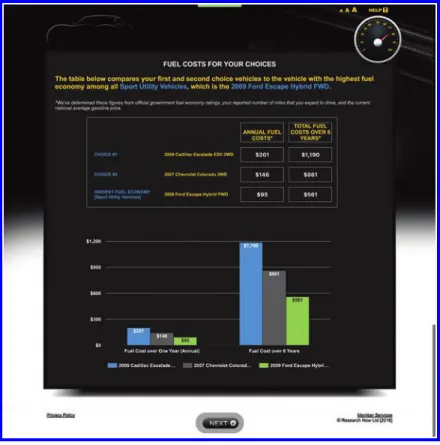
The ResearchNow computers assigned 60 percent of people to treatment and 40 percent to control using an algorithm that we discuss below. The base treatment was to provide information similar to the dealership experiment tablet app, including annual and “lifetime” (over the expected years of ownership) costs for the first-choice and second-choice vehicles, as well as for the highest-MPG vehicle in the same class as the first choice. Figure 3 presents a picture of the key information treatment screen. As in the dealership experiment, we compared these fuel costs to other tangible purchases: “that’s the same as it would cost for 182 gallons of milk” or for “16 weeks of lunch.”
Because we had fully computerized experimental control instead of delivering the treatment through RAs, we decided to implement four information treatment arms instead of just one. The “Base Only” treatment included only the above information, while the other three treatments included additional information. The “Base + Relative” treatment used the self-reported average weekly mileage to compare fuel savings to those that would be obtained at the national average mileage of about 12,000 miles per year. The “Base + Climate” treatment compared the social damages from carbon emissions (monetized at the social cost of carbon) for the same three vehicles as in the Base sub-treatment. The “Full” treatment included all of the Base, Relative, and Climate treatments. There were also four control groups, each of which paralleled one of the treatment arms in length, graphics, and text, but contained placebo information that was unrelated to fuel economy and would not plausibly affect purchases.6
To ensure that people engaged with and understood the information, participants were given a four-part multiple choice question after each of the treatment and control screens. For example, after the base treatment screen in Figure 3, participants were asked, “What is the difference in total fuel costs over [self-reported own-ership period] years between the best-in-class MPG model and your first choice
6 The Base control group was informed about worldwide sales of cars and commercial vehicles in 2007, 2010,
and 2013. The second control group received the Base information plus information on average vehicle-miles traveled in 2010 versus 1980. The third control group received the Base information plus data on the number of cars, trucks, and buses on the road in the United States in 1970, 1990, and 2010. The fourth control group received all control information.
vehicle?” Four different answers were presented, only one of which matched the information on the previous screen. Sixty-nine, 79, and 79 percent of the treatment group answered the Base, Relative, and Environment quiz questions correctly on the first try. Seventy-seven, 66, and 84 percent of the control group answered the three control group quiz questions correctly on the first try. Every participant was required to answer the questions correctly before advancing.
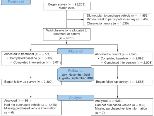
Figure 4 presents a Consort diagram for the online experiment. The baseline survey and intervention were delivered in March 2015. We conducted the follow-up surveys in two rounds, the first from July to November 2015 and the second in August and September 2016. Here, 6,316 people planned to purchase vehicles and agreed to participate in the survey, of whom 5,014 finished the baseline sur-vey and treatment or control intervention. There is natural attrition over time in the ResearchNow panel, and 3,867 people began the follow-up survey when it was fielded. Of those who began the follow-up survey, 2,378 had not bought a new vehi-cle or had incomplete data, leaving a final sample of 1,489 people for our treatment effect estimates.
Figure 3. Online Treatment Screen
Notes: This is a screen capture from part of the online informational intervention. Choices #1 and #2 were the participant’s first-choice and second-choice vehicles, and fuel costs were based on self-reported driving patterns and expected gas prices.
II. Sample Characteristics
A. Summary Statistics
Table 1 presents summary data for the samples that began the dealership and online experiments —specifically, the samples of valid observations that were randomized into treatment or control. For the dealership experiment, age, gender, and race were coded by the RAs at the end of the tablet survey, and income is the median income in the consumer’s zip code. For the online experiment, demographics are from basic demographics that the respondent provided to ResearchNow upon entering the panel. We impute missing covariates with sample means. See online Appendix A for additional details on data preparation.
Given that the dealership sample was recruited at Ford dealerships, it is not surprising that 40 percent of that sample currently drove a Ford, and 67 percent eventually purchased a Ford. By contrast, 12 percent of the online sample currently drove a Ford, and 11 percent purchased a Ford, closely consistent with the national average.
Fuel intensity (in gallons per mile (GPM)) is the inverse of fuel economy (in miles per gallon). For readability, we scale fuel intensity in gallons per 100 miles. The average vehicles use 4 to 5 gallons per 100 miles, meaning that they get 20 to 25 miles per gallon. We carry out our full analysis using fuel intensity instead of fuel economy because fuel costs are a key eventual outcome, and fuel costs scale
Allocated to treatment (n = 3,771) • Completed baseline (n= 3,109) ◦ Completed intervention (n= 3,011) Allocated to control (n= 2,545) • Completed baseline (n= 2,093) ◦ Completed intervention (n= 2,003) Enrollment Began survey (n = 23,203) March 2015
Valid observations allocated to treatment or control
(n= 6,316)
Did not plan to purchase vehicle (n = 14,855) Did not want to participate in survey (n = 402) Observation errors (n= 1,630)
Allocation
Analyzed (n= 861)
Had not purchased vehicle (n= 1,435) Missing purchased vehicle information (n= 6)
Analyzed (n= 628)
Had not purchased vehicle (n= 930) Missing purchased vehicle information (n = 7)
Analysis Follow-up
July–November 2015 August– September 2016
Began follow-up survey (n= 2,302) Began follow-up survey (n= 1,565)
linearly in GPM. “Consideration set fuel intensity” is the mean fuel intensity in the consumer’s consideration set.7
The final row reports that 67 to 68 percent of vehicle purchases in the two experiments were “new,” as defined by having a model year of 2013 or later (in the dealership experiment) or 2015 or later (in the online experiment). The third column in Table 1 presents the same covariates for the national sample of new car buyers from the 2009 National Household Travel Survey (NHTS), weighted by the NHTS sample weights. For the NHTS, we define “new car buyers” as people who own a model year 2008 or later vehicle in the 2009 survey. Unsurprisingly, neither of our samples is representative of the national population of new car buyers. Interestingly, however, they are selected in opposite ways for some covariates: the online sample is slightly older, significantly wealthier, and drives less than the national comparison
7 A small share of vehicles (0.2 to 0.3 percent of purchased and first choice vehicles) are electric. For electric
vehicles, the EPA calculates MPG equivalents using the miles a vehicle can travel using the amount of electricity that has the same energy content as a gallon of gasoline. We omit electric vehicles from the descriptive analyses of gasoline cost beliefs, but we include electric vehicles in the treatment effect estimates.
Table 1— Comparison of Sample Demographics to National Averages Dealership
sample
Online sample
National (new car buyers)
(1) (2) (3) Male 0.64 0.60 0.48 (0.47) (0.49) (0.26) Age 41.37 54.83 54.01 (12.87) (13.64) (13.14) White 0.77 0.86 0.91 (0.41) (0.35) (0.29) Income ($000s) 73.51 121.93 82.08 (25.69) (138.33) (35.68)
Miles driven/year (000s) 15.29 11.68 13.38
(11.80) (7.94) (9.91)
Current vehicle is Ford 0.40 0.12 0.11
(0.48) (0.32) (0.31)
Current fuel intensity
(gallons/100 miles) (1.15)4.70 (1.08)4.57 (1.50)4.58
Consideration set fuel intensity
(gallons/100 miles) (1.20)4.35 (0.96)4.15 —
Purchased fuel intensity
(gallons/100 miles) (1.26)4.34 (1.00)4.08 — Purchased new/ late-model vehicle 0.67 0.68 — (0.47) (0.47) Observations 1,989 6,316 18,053
Notes: This table shows sample means, with standard deviations in parentheses. The first two columns are the samples of valid observations that were randomized into treatment or control in the dealership and online experiments, respectively. “Purchased new/late-model vehicle” is an indicator for whether the purchased vehicle is model year 2013 (2015) or later in the dealership (online) sample. The national sample is the sample of households with model year-2008 or later vehicles in the 2009 National Household Travel Survey (NHTS), weighted by the NHTS sample weights.
group, while the dealership sample is younger, less wealthy, and drives more than the national population.
For some regressions, we re-weight the final samples to be nationally representative on observables using entropy balancing (Hainmueller 2012). We match sample and population means on the six variables in Table 1 that are available in the NHTS: gender, age, race (specifically, a White indicator variable), income, miles driven per year, whether the current vehicle is a Ford, and current vehicle fuel intensity. By construction, the mean weight is one. For the dealership and online samples, respectively, the standard deviations of weights across observations are 1.28 and 0.73, and the maximum observation weights are 12.0 and 9.2.
B. Balance and Attrition
ResearchNow allocated observations to the four treatment and four control groups using a modification of the least-fill algorithm.8 In the standard least-fill
algorithm, a survey respondent is allocated to the group with the smallest number of completed surveys. A treatment or control group closes when it reaches the requested sample size, and the survey closes when the last group is full. In this algorithm, between the times when the groups close, group assignment is arbitrary and highly likely to be exogenous, as it depends only on an observation’s exact arrival time. Over the full course of the survey, however, group assignment may be less likely to be exogenous, as some treatment or control groups close before others, and different types of people might take the survey earlier versus later. To address this possible concern, we condition regressions on a set of “treatment group closure time indicators,” one for each period between each group closure time.9 While we
include these indicators to ensure that it is most plausible to assume that treatment assignment is unconfounded, it turns out that their inclusion has very little impact on the results.
The first eight variables in Table 1 were determined before the information treatment was delivered. Online Appendix Table A2 shows that F-tests fail to reject that these eight observables are jointly uncorrelated with treatment status. In other words, treatment and control groups are statistically balanced on observables. By chance, however, several individual variables are unbalanced at conventional levels of statistical significance: current vehicle and consideration set fuel intensity in the dealership experiment, and income in the online experiment. We use the eight predetermined variables as controls to reduce residual variance and ensure condi-tional exogeneity in treatment effect estimates.
As we had expected, attrition rates are high. However, this does not appear to threaten internal validity. Online Appendix Table A3 shows that attrition rates are
8 We had instructed ResearchNow to use random assignment, but they did not do this, and we did not discover
the discrepancy until we analyzed the data.
9 We say a “modification” of the least-fill algorithm because there were also some deviations from the above
procedure. In particular, had the procedure been followed exactly, the last 20 percent of surveys would all be assigned to a treatment group, as 60 percent of observations were assigned to treatment versus 40 percent for control. However, ResearchNow modified the algorithm in several ways, and we thus have both treatment and control observations within each of the treatment group closure time indicators.
balanced between treatment and control groups in both experiments, and online Appendix Table A4 shows that attrition rates in treatment and control do not differ on observables. On the basis of these results, we proceed with the assumption that treatment assignment is unconfounded.
III. Consideration Sets
Before presenting results in Section IV, we first present data that help to understand the possible scope for fuel economy information to affect purchases. We first study the variation in fuel economy within each consumer’s consideration set, as well as the probability that consumers eventually purchase a vehicle from the consideration set instead of some other vehicle that was not in the consideration set. If consideration sets have little variation and consumers mostly buy vehicles from their consideration sets, this suggests that there will be little scope for the information treatments to affect purchased vehicle fuel economy. On the other hand, if consideration sets have substantial variation in fuel economy, or if consumers often buy vehicles from outside their consideration sets, this suggests that there could be significant scope for the treatments to affect purchases.
We then study the extent to which consumers report incorrect beliefs about fuel costs for vehicles in their consideration sets. If consumers’ fuel cost beliefs are already largely correct, this suggests that there is little need for additional information. If consumers’ fuel cost beliefs are noisy but unbiased, this suggests that information provision could increase allocative efficiency but might not affect average fuel economy of vehicles purchased. If consumers systematically overestimate ( underestimate) fuel costs, this suggests that information provision could decrease (increase) the average fuel economy of vehicles purchased.
A. Characterizing Consideration Sets
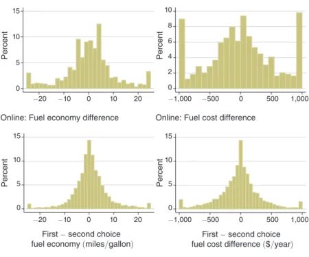
Figure 5 presents information on the fuel economy variation in consumers’ consideration sets, with the dealership and online experiments on the top and bottom, respectively. The left two panels show the distributions of MPG differences between consumers first- and second-choice vehicles. For the right two panels, we define G ij⁎ as the annual fuel cost for consumer i in vehicle j , given the vehicle’s fuel economy rating and the consumer’s self-reported miles driven, city versus highway share, and per gallon gasoline price. The right two panels present the distribution of fuel cost differences between first- and second-choice vehicles, i.e., G i⁎1 − G i⁎2 .
All four histograms demonstrate substantial variation fuel economy in consumers’ consideration sets. This implies that there could be significant scope for fuel economy information to affect purchased vehicle fuel economy, even if all consumers were to choose only from the consideration sets they reported at baseline.
The top part of Table 2 compares consumers’ eventual purchases to the vehicles they were considering at baseline. In the dealership and online experiments, respectively, 49 and 35 percent of consumers ended up purchasing a vehicle of the same make and model as either the first or second choice from the baseline survey. In the dealership experiment, 73 percent of people purchased vehicles of the same
make as one of the two vehicles in their consideration set; this high proportion is unsurprising given that the participants were recruited from Ford dealerships. The final row of that part of the table shows a strong correlation between consideration set average fuel intensity and purchased vehicle fuel intensity.
The bottom part of Table 2 presents basic facts about the variation in fuel economy within consumers’ consideration sets. The first row shows that the average consumers in the dealership and online experiments, respectively, were considering two vehicles that differed by 8.5 and 5.4 miles per gallon, or 1.1 and 0.7 gallons per 100 miles. The third row shows that the average consumers in the two experiments would have increased fuel economy by 3.9 and 2.3 MPG by switching from the first-choice vehicle to the vehicle with the highest MPG in the consideration set. This is about half of the previous number because for about half of consumers, the first-choice vehicle already is the highest-MPG vehicle in the consideration set. Finally, the average consumers in the two experiments were considering two vehicles with fuel costs that differed by $523 and $245 per year, at their self-reported miles driven, city versus highway share, and per gallon gasoline price.
Figure 5. Distributions of Annual Fuel Cost Differences between First- and Second-Choice Vehicles
Notes: The left two histograms present the distributions of fuel economy differences between consumers’ first- and second-choice vehicles. The right two histograms present the distributions of fuel cost differences between consumers’ first- and second-choice vehicles, given the vehicles’ fuel economy ratings and consumers’ self-reported miles driven, city versus highway share, and per gallon gasoline price. Outlying observations are collapsed into the outermost bars. 0 5 10 15 Percent −20 −10 0 10 20 −20 −10 0 10 20 Dealership: Fuel economy difference
0 2 4 6 8 10 Percent Percent Percent −1,000 −500 0 500 1,000 −1,000 −500 0 500 1,000 Dealership: Fuel cost difference
0 5 10 15
First − second choice fuel economy (miles/gallon) Online: Fuel economy difference
0 5 10 15
First − second choice fuel cost difference ($/year) Online: Fuel cost difference
While there is considerable variation within consideration sets, this is of course still smaller than the variation between consumers. In the dealership experiment consideration sets, the within- and between-consumer standard deviations in fuel economy are 6.5 and 9.7 MPG, respectively. For the online experiment consideration sets, the within- and between-consumer standard deviations are 5.0 and 8.7 MPG, respectively.
B. Beliefs about Consideration Set Fuel Costs
Above, we described the actual fuel costs for vehicles in consumers’ consideration sets. We now examine a different question: what were consumers’ beliefs about fuel costs? To do this, we follow Allcott (2013) in constructing “valuation ratios.” We define G ̃ ij as consumer i ’s belief about annual gas costs of vehicle j , as elicited in the baseline survey. As above, G ij⁎ is the “true” value given the vehicle’s fuel economy rating and the consumer’s self-reported miles driven, city versus highway share, and per-gallon gasoline price. For a given vehicle j , consumer i ’s valuation ratio is the share of the true fuel cost that is reflected in beliefs:
(1) ϕ ij =
G ̃ ij
___
G ij⁎ .
Table 2— Consideration Sets
Dealership experiment
Online experiment
(1) (2)
Panel A.Consideration sets versus final purchases
Share with …
purchased model = first-choice model 0.42 0.30
purchased make = first-choice make 0.70 0.53
purchased model = second-choice model 0.12 0.06
purchased make = second-choice make 0.70 0.25
purchased model = first- or second-choice model 0.49 0.35
purchased make = first- or second-choice make 0.73 0.63
Correlation between consideration set average MPG
and purchased MPG 0.52 0.44
Panel B. Variation in consideration sets
Average of …
|first-choice − second-choice MPG| 8.5 5.4
|first-choice − second-choice gallons/100 miles| 1.1 0.7
max {consideration set MPG} − First-choice MPG 3.9 2.3
max {consideration set gallons/100 miles} −
First-choice gallons/100 miles 0.59 0.39
|first-choice − second-choice fuel cost| ($/year) 523 245
Notes: Panel A of this table compares consideration sets (first- and second-choice vehicles) from the baseline surveys with the purchased vehicles reported in the follow-up surveys. Panel B presents variation in fuel economy and fuel costs within consumers’ consideration sets.
For any pair of vehicles j ∈ {1, 2} , consumer i ’s valuation ratio is the share of the true fuel cost difference that is reflected in beliefs:
(2) ϕ i =
G ̃ i1 − G ̃ i2
________
G i⁎1 − G i⁎2 .
For both ϕ ij and ϕ i , the correct benchmark is ϕ = 1 . Note, ϕ > 1 if the con-sumer perceives larger fuel costs, and ϕ < 1 if the consumer perceives smaller fuel costs. Larger
|
ϕ − 1|
reflects more “noise” in beliefs.For example, consider two vehicles, one that gets 25 MPG (4 gallons per 100 miles) and another that gets 20 MPG (5 gallons per 100 miles). For a consumer who expects to drive 10,000 miles per year with a gas price of $3 per gallon, the two cars would have “true” annual fuel costs G i⁎1 = $1,200 and G i⁎2 = $1,500 . If on the survey, the consumer reports G ̃ i1 = $1,400 and G ̃ i2 = $1,250 , we would calculate ϕ i = 1,400 − 1,250__________1,500 − 1,200 = 0.5 . In other words, the consumer responds as if she recognizes only half of the fuel cost differences between the two vehicles.
The fuel cost beliefs elicited in the surveys are a combination of consumers’ actual beliefs plus some survey measurement error. Survey measurement error is especially important due to rounding (most responses are round numbers) and because we did not incentivize correct answers.10 Online Appendix Table A6, however, shows that
elicited beliefs appear to be meaningful, i.e., not just survey measurement error: the results suggest both that ϕ ij , ϕ i , and
|
ϕ i − 1|
are correlated within individual between the baseline and follow-up surveys, and that people who perceive larger fuel cost differences (higher ϕ i ) also buy higher MPG vehicles, although the results from the dealership experiment are imprecise due to the smaller sample.Figure 6 presents the distributions of valuation ratios in the baseline dealership and online surveys. The left panels show ϕ ij from equation (1) for the first-choice vehicles, while the right panels show ϕ i from equation (2) for the first- versus second-choice vehicles. Since there can be significant variation in ϕ i , especially for two vehicles with similar fuel economy, we winsorize to the range − 1 ≤ ϕ ≤ 4 .11
The figure demonstrates three key results. First, people’s reported beliefs are very noisy. Perfectly reported beliefs would have a point mass at ϕ = 1 . In the dealership and online experiments, respectively, 24 and 32 percent of ϕ ij in the left panels are off by a factor of two or more, i.e., ϕ ij ≤ 0.5 or ϕ ij ≥ 2 . This reflects some combination of truly noisy beliefs and survey reporting error.
Second, many people do not correctly report whether their first- or second-choice vehicle has higher fuel economy, let alone the dollar value of the difference in fuel costs. Forty-five and 59 percent of respondents in the dealership and online data, respectively, have ϕ i = 0 , meaning that they reported the same expected fuel costs for vehicles with different fuel economy ratings. In both surveys, 8 percent have
10 Allcott (2013) shows that incentivizing correct answers does not affect estimates of belief errors in a related
context.
11 In the dealership experiment, this winsorization affects 5.2 and 13.2 percent of the observations of ϕ
ij and ϕ i ,
ϕ i < 0 , meaning that they have the MPG rankings reversed. Thus, in the dealership
and online surveys, respectively, only 47 and 33 percent of people correctly report which of their first- versus second-choice vehicle has higher fuel economy. This result also reflects some combination of incorrect beliefs and survey reporting error.
Third, it is difficult to argue conclusively whether people systematically overstate or understate fuel costs. The thin vertical lines in Figure 6 mark the median of each distribution. The top left figure shows that the median person in the dealership survey overestimated fuel costs by 20 percent ( ϕ ij = 1.2 ), which amounts to approximately $200 per year. The median person in the online survey, by contrast, has ϕ ij = 0.99 . In the histograms on the right, the median ϕ i is zero in both surveys, reflecting the results of the previous paragraph. All four histograms show significant dispersion, making the means harder to interpret.
IV. Empirical Results
We estimate the effects of information by regressing purchased vehicle fuel intensity on a treatment indicator, controlling for observables. Define Y i as the fuel intensity of the vehicle purchased by consumer i , measured in gallons per 100 miles. Define T i as a treatment indicator, and define X i as a vector of controls for the eight predetermined variables in Table 1: gender, age, race, natural log of income, miles
Figure 6. Distributions of Fuel Cost Beliefs: Valuation Ratios
Notes: These figures present the distribution of valuation ratios in the baseline surveys for the dealership and online experiments. The left panels present the valuation ratio from equation (1) for the first-choice vehicles. The right panels present the valuation ratios from equation (2) for the first- versus second-choice vehicles. In the right panels, a valuation ratio of zero means that the consumer reported the same expected fuel costs for both vehicles.
0 2 4 6 8 10 Percent 0 1 2 3 4
Dealership: First choice
0 10 20 30 40 50 Percent −1 0 1 2 3 4
Dealership: First − second choice
0 2 4 6 8 10 Percent 0 1 2 3 4
Fuel cost valuation ratio Online: First choice
0 20 40 60 Percent −1 0 1 2 3 4
Fuel cost valuation ratio Online: First − second choice
driven per year, an indicator for whether the current vehicle is a Ford, current vehicle fuel intensity, and consideration set average fuel intensity. The latter two variables soak up a considerable amount of residual variance in Y i . For the online experiment,
X i also includes the treatment group closure time indicators. The primary estimating
equation is
(3) Y i = τ T i + β X i + ε i .
We first study effects on stated preference questions in the online experiment, both immediately after the intervention and in the follow-up survey. The immediate stated preference questions are useful because they show whether the intervention had any initial impact. By comparing effects on the exact same questions asked months later during the follow-up, we can measure whether the intervention is forgotten. We then estimate effects on the fuel economy of purchased vehicles, for the full sample and then for subgroups that might be more heavily affected.
A. Effects on Stated Preference in the Online Experiment
We first show immediate effects on stated preference questions asked just after the online intervention. To increase power, we use the full sample available from the baseline survey, which includes many participants who do not appear in the follow-up survey. Table 3 reports results for three sets of questions. Panel A reports estimates of equation (3) where the dependent variable is the response to the ques-tion, “How important to you are each of the following features? (Please rate from 1–10, with 10 being “most important.)” Panel B reports estimates where the depen-dent variable is the answer to the question, “Imagine we could take your most likely choice, the [first-choice vehicle], and change it in particular ways, keeping every-thing else about the vehicle the same. How much additional money would you be willing to pay for the following?” In both panels, the feature is listed in the column header. Panel C presents the expected fuel intensity, i.e., weighted average of the first- and second-choice vehicles, weighted by the post-intervention reported pur-chase probability. In panel C, the R 2 is very high, and the estimates are very precise.
This is because X i includes the consideration set average fuel intensity, which is the same as the dependent variable except that it is not weighted by post-intervention reported purchase probability.
Results in panels A and B show that the information treatment actually reduced the stated importance of fuel economy. The treatment group rated fuel economy 0.56 points less important on a scale of 1–10 and was willing to pay $92.18 and $237.96 less for five and 15 MPG fuel economy improvements, respectively. The treatment also reduced the stated importance of price, although the effect size is less than half of the effect on fuel economy. Preferences for power, leather interior, and sunroof are useful placebo tests, as the intervention did not discuss these issues. As expected, there are no effects on preferences for these attributes.12
12 We thank a referee for pointing out that a WTP of only $242 for a one-second improvement in 0–60 time
Why might the intervention have reduced the importance of fuel economy? One potential explanation is that people initially overestimated fuel costs and fuel cost differences, and the quantitative information in the treatment helps to correct these biased beliefs. As we saw in Figure 6, however, there is no clear evidence that this is the case for the online experiment sample. Furthermore, we can calculate the
usual concerns about taking unincentivized stated preference questions too seriously; our main focus is the effects on actual purchases in Tables 5 and 6.
Table 3—Immediate Effect of Information on Stated Preference in Online Experiment
Power Fuel economy Price Leather interior Sunroof (1) (2) (3) (4) (5)
Panel A. Importance of features, from 1 (least important) to 10 (most important)
Treatment −0.04 −0.56 −0.24 −0.06 0.10
(0.06) (0.06) (0.05) (0.09) (0.08)
Observations 5,036 5,036 5,036 5,036 5,036
R 2 0.04 0.13 0.06 0.07 0.04
Dependent variable mean 6.62 7.68 8.31 4.65 3.80
Leather interior 5 MPG improvement 15 MPG improvement Power: 0–60 MPH 1 second faster (1) (2) (3) (4)
Panel B. Willingness-to-pay for additional features
Treatment 4.49 −92.18 −237.96 16.89
(16.77) (15.81) (35.14) (19.35)
Observations 4,609 4,512 4,512 4,609
R 2 0.06 0.06 0.07 0.05
Dependent variable mean 380 409 1,043 242
Expected fuel intensity (gallons/100 miles)
(1) Panel C. Expected fuel intensity
Treatment −0.032
(0.004)
Observations 5,018
R 2 0.97
Dependent variable mean 4.12
Notes: This table presents estimates of equation (3). The dependent variables in panel A are responses to the
ques-tion, “How important to you are each of the following features? (Please rate from 1–10, with 10 being “most
important).” Dependent variables in panel B are responses to the question, “Imagine we could take your most likely choice, the [first choice vehicle], and change it in particular ways, keeping everything else about the vehicle the same. How much additional money would you be willing to pay for the following?” In both panels, the feature is listed in the column header. In panel C, the dependent variable is the weighted average fuel intensity (in gallons per 100 miles) of the two vehicles in the consideration set, weighted by post-intervention stated purchase probability. Data are from the online experiment, immediately after the treatment and control interventions. All columns control for gender, age, race, natural log of income, miles driven per year, an indicator for whether the current vehicle is a Ford, current vehicle fuel intensity, consideration set average fuel intensity, and treatment group closure time indicators. Robust standard errors are in parentheses.
actual annual savings from 5 and 15 MPG fuel economy improvements given each consumer’s expected gasoline costs and driving patterns and the MPG rating of the first-choice vehicle. The control group has average willingness-to-pay of $464 and $1,186 for 5 and 15 MPG improvements, respectively. The actual annual savings are $266 and $583. This implies that the control group requires a remarkably fast pay-back period—approximately two years or less—for fuel economy improvements. It therefore seems unlikely that the control group overestimated the value of fuel econ-omy improvements. Notwithstanding, the results in panels A and B are very robust: for example, they are not driven by outliers, and they don’t depend on whether or not we include the control variables X i .
Panel C of Table 3 shows that the treatment shifted purchase probabilities toward the higher MPG vehicle in consumers’ consideration set. This effect is small: a 25-MPG car has a fuel intensity of 4 gallons per 100 miles, so a decrease of 0.032 represents only a 0.8 percent decrease. In units of fuel economy, this implies moving from 25 to 25.2 miles per gallon.
It need not be surprising that the intervention shifted stated preference toward higher MPG vehicles in the consideration set while also reducing the stated gen-eral importance of fuel economy. As we saw in Figure 6, about two-thirds of online survey respondents do not correctly report which vehicle in their consid-eration set has higher MPG. Thus, even if the treatment makes fuel economy less important in general, it is still a positive attribute, and the treatment can shift pref-erences toward higher-MPG vehicles by clarifying which vehicles are in fact higher MPG. Furthermore, even consumers who do correctly report which vehicle in their consideration has lower fuel costs may be uncertain, and the treatment helps make them more certain.
We also asked the same stated preference questions from panels A and B on the follow-up survey, which respondents took 4 to 18 months later. Table 4 parallels panels A and B of Table 3, but using these follow-up responses. Only one of the nine variables (importance of price from 1–10) demonstrates an effect that is statistically significant with 90 percent confidence. For the fuel economy variables, there are zero remaining statistical effects, and we can reject effects of the sizes reported in Table 3. This suggests that the effects of information wear off over time, perhaps as people forget.
B. Effects on Vehicle Purchases
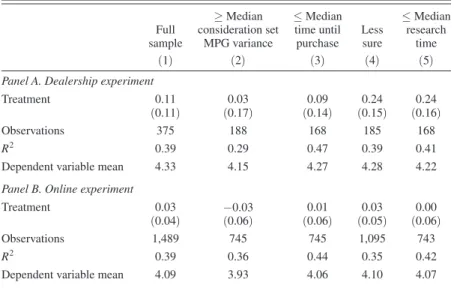
Did the interventions affect only stated preference, or did they also affect actual purchases? Table 5 presents treatment effects on the fuel intensity of purchased vehicles. Columns 1–3 present dealership experiment results, while columns 4 – 6 present online experiment results. Columns 1 and 4 omit the X i variables, while columns 2 and 5 add X i ; the point estimates change little. Columns 3 and 6 are
weighted to match US population means, as described in Section II. In all cases, information provision does not statistically significantly affect the average fuel intensity of the vehicles consumers buy.
The bottom row of Table 5 presents the lower bounds of the 90 percent confidence intervals of the treatment effects. Put simply, these are the largest
statistically plausible effects of information on fuel economy. With equally weighted observations in columns 2 and 5, the confidence intervals rule out fuel intensity decreases of 0.06 and 0.04 gallons per 100 miles in the dealership and
Table 4 — Effect of Information on Stated Preference in Online Experiment Follow-up Survey
Power Fuel economy Price Leather interior Sunroof (1) (2) (3) (4) (5)
Panel A. Importance of features, from 1 (least important) to 10 (most important)
Treatment 0.12 −0.10 −0.17 0.15 0.07
(0.12) (0.11) (0.10) (0.17) (0.16)
Observations 1,542 1,544 1,543 1,542 1,541
R 2 0.03 0.07 0.03 0.05 0.03
Dependent variable mean 6.90 7.76 8.49 4.95 4.02
Leather
interior improvement5 MPG improvement15 MPG Power: 0–60 MPH 1 second faster
(1) (2) (3) (4)
Panel B. Willingness-to-pay for additional features
Treatment −37.41 2.66 20.31 13.48
(29.38) (23.97) (56.25) (27.76)
Observations 1,359 1,329 1,329 1,359
R 2 0.06 0.04 0.04 0.03
Dependent variable mean 316 346 940 168
Notes: This table presents estimates of equation (3). The dependent variables in panel A are responses to the ques-tion, “How important to you are each of the following features? (Please rate from 1–10, with 10 being “most import-ant).” Dependent variables in panel B are responses to the question, “Imagine we could take your most likely choice, the [first choice vehicle], and change it in particular ways, keeping everything else about the vehicle the same. How much additional money would you be willing to pay for the following? ” In both panels, the feature is listed in the column header. Data are from the follow-up survey for the online experiment. All columns control for gender, age, race, natural log of income, miles driven per year, an indicator for whether the current vehicle is a Ford, current vehicle fuel intensity, consideration set average fuel intensity, and treatment group closure time indicators. Robust standard errors are in parentheses.
Table 5—Effects of Information on Fuel Intensity of Purchased Vehicles
Dealership Online
(1) (2) (3) (4) (5) (6)
Treatment 0.07 0.11 −0.21 0.05 0.03 0.01
(0.13) (0.11) (0.17) (0.05) (0.04) (0.06)
90% confidence interval lower bound −0.15 −0.06 −0.49 −0.03 −0.04 −0.08
Observations 375 375 375 1,489 1,489 1,489
R 2 0.00 0.39 0.29 0.00 0.39 0.38
Dependent variable mean 4.33 4.33 4.33 4.09 4.09 4.09
Controls No Yes Yes No Yes Yes
Weighted No No Yes No No Yes
Notes: This table presents estimates of equation (3). The dependent variable is the fuel intensity (in gallons per 100 miles) of the vehicle purchased. All columns control for gender, age, race, natural log of income, miles driven per year, an indicator for whether the current vehicle is a Ford, current vehicle fuel intensity, and consideration set average fuel intensity. Columns 4–6 also control for treatment group closure time indicators. Samples in columns 3 and 6 are weighted to match the national population of new car buyers.