Ionomer self-assembly in dilute solution studied by coarse-grained molecular dynamics

Publisher’s version / Version de l'éditeur:

Macromolecules, 49, 4, pp. 1479-1489, 2016-02-02

READ THESE TERMS AND CONDITIONS CAREFULLY BEFORE USING THIS WEBSITE.

https://nrc-publications.canada.ca/eng/copyright

Vous avez des questions? Nous pouvons vous aider. Pour communiquer directement avec un auteur, consultez la première page de la revue dans laquelle son article a été publié afin de trouver ses coordonnées. Si vous n’arrivez pas à les repérer, communiquez avec nous à PublicationsArchive-ArchivesPublications@nrc-cnrc.gc.ca.

Questions? Contact the NRC Publications Archive team at

PublicationsArchive-ArchivesPublications@nrc-cnrc.gc.ca. If you wish to email the authors directly, please see the first page of the publication for their contact information.

NRC Publications Archive

Archives des publications du CNRC

This publication could be one of several versions: author’s original, accepted manuscript or the publisher’s version. / La version de cette publication peut être l’une des suivantes : la version prépublication de l’auteur, la version acceptée du manuscrit ou la version de l’éditeur.

For the publisher’s version, please access the DOI link below./ Pour consulter la version de l’éditeur, utilisez le lien DOI ci-dessous.

https://doi.org/10.1021/acs.macromol.5b02158

Access and use of this website and the material on it are subject to the Terms and Conditions set forth at

Ionomer self-assembly in dilute solution studied by coarse-grained

molecular dynamics

Ghelichi, Mahdi; Malek, Kourosh; Eikerling, Michael H.

https://publications-cnrc.canada.ca/fra/droits

L’accès à ce site Web et l’utilisation de son contenu sont assujettis aux conditions présentées dans le site LISEZ CES CONDITIONS ATTENTIVEMENT AVANT D’UTILISER CE SITE WEB.

NRC Publications Record / Notice d'Archives des publications de CNRC:

Ionomer Self-Assembly in Dilute Solution Studied by Coarse-Grained

Molecular Dynamics

Mahdi Ghelichi,

Kourosh Malek,

and Michael H. Eikerling

*

†

Department of Chemistry, Simon Fraser University, 8888 University Drive, Burnaby, BC V5A 1S6, Canada

‡

Energy, Mining, and Environment, National Research Council of Canada, 4250 Wesbrook Mall, Vancouver, BC V6T 1W5, Canada ABSTRACT: Coarse-grained molecular dynamics simulations,

reported in this article, elucidate the self-assembly of semiflexible ionomer molecules into cylindrical bundle-like aggregates. Ionomer chains are composed of hydrophobic backbones, grafted with pendant side chains that are terminated by anionic headgroups. Bundles have a core of backbones surrounded by a surface layer of charged anionic headgroups and a diffuse halo of counterions. Parametric studies of bundle properties unravel the interplay of backbone hydrophobicity, strength of electrostatic interactions between charged moieties, side chain content, and counterion valence: expectedly, the size of bundles increases with backbone

hydrophobicity; the aggregate size depends nonmonotonically on the Bjerrum length; increasing the grafting density of pendant side chains results in smaller bundles; and the counterion valence exerts a strong effect on bundle size and counterion localization in the near-bundle region. Results reveal how the ionomer architecture and solvent properties influence the ionomer aggregation and associated electrostatic and mechanical bundle properties. These properties of ionomer aggregates are vital for rationalizing the water sorption behavior and transport phenomena as well as the chemical and mechanical stability of ionomer membranes.

■

Ionomers are moderately charged polymers with an ion content of approximately 15 mol % with respect to the amount of polymer repeat units of the backbone. The molecular architecture of ionomer moieties, ionomer density, and solvent properties determine the strengths of hydrophobic, dipolar, and ionic interactions in these systems. The interplay of these interactions results in a rich variety of structural conformations that can be classified as solution, hydrated, and melt forms. Ionomer solutions find application in paint suspensions and coating materials.1,2 The hydrated state is encountered in electrochemical cells such as chlor-alkali cells, redox flow batteries, and polymer electrolyte fuel cells (PEFCs), where the ionomer needs to provide highly efficient and selective proton or ion transport.3,4 Ionomer melts find major applications in battery electrolytes but also in coating technologies.4,5

In low-polarity solvents,1,2 association of acid headgroups occurs due to dipolar interactions that form ionic multiples. In high-polarity solvents, acidic groups dissociate completely leading to two types of ionomer behavior based on the strength of polymer−solvent interactions. Under good solvent conditions for the polymer backbone, i.e., in a solvent that dissolves the backbone chains, solvated ionomer molecules exhibit polyelectrolyte-type behavior, forming loose ionic aggregates. In sufficiently polar solvents, ionomer backbones undergo aggregation and phase separation. This process results in the formation of a solid polymer electrolyte membrane (PEM) at high ionomer concentration.6

The best known PEM materials that are employed in PEFCs and PEM electrolyzers belong to the family of perfluorosulfonic acid (PFSA) ionomers, such as the famous Nafion of DuPont.6,7 These materials consist of a strongly hydrophobic backbone with the chemical structure of Teflon and randomly attached pendant side chains of perfluorinated vinyl ethers. Side chains are terminated with sulfonic acid headgroups that are similar in acid strength to trifluoromethanesulfonic acid (“triflic” acid).8 Under sufficiently hydrated conditions, PEMs exhibit high mechanical robustness, warranted by apolar backbone segments, as well as good water retention and high proton conductivity, conferred by the high volumetric ion density.

Studies of the structure of Nafion and assorted materials have primarily focused on the solid membrane state (with water volume fraction significantly below 50%). Using a large variety of experimental techniques, a suite of structural models have been proposed, including parallel cylinder model,9 cluster-channel model,10,11_lamellar12,13_{or skin-type model,}14_{and rod} network model.15,16 _{However, none of these simplified} modelistic views captures the realistic membrane structure. From a fundamental perspective, solution studies of ionomer aggregation should be highly insightful in this regard.

Based on SAXS, SANS, ESR, and 19_{F NMR}

experi-ments,17−22 _{it was conjectured that hydrophobic backbones}

Received: September 30, 2015 Revised: November 27, 2015 Published: February 2, 2016

of Nafion form the core of self-assembled ionomer structures while ionic units are located at the periphery of this configuration. Jiang et al.21employed dynamic light scattering (DLS) to study the self-assembly of Nafion chains in dilute aqueous solution. Observation of stable aggregates supported the fringed-rod ionomer model proposed by Szajdzinska-Pietek et al.23,24 _{These structures are similar in nature to the} cylindrical-like micelles formed in solutions of semirigid synthetic polyelectrolytes such as sulfonated poly(p-phenyl-ene).25−27 Loppinet, Gebel, and others19,20,28 studied the influence of various parameters on the self-assembling behavior in ionomer solutions. They observed that the dielectric constant of the solvent and the grafting density of pendant side chains influence the size of ionomer bundles. Using a combination of scattering and microscopy, Rubatat et al.15,16,29 provided evidence of fibrillar (rodlike) aggregates in well-hydrated PEMs. The proton conductivity and mechanical strength of solution-cast membranes, formed from different solvents, were correlated with the properties of polymeric bundles formed in Nafion solutions.30 Rod-like bundles have also been reported for hydrated sulfonated polyphenylene ionomers.31 Recent studies identified aggregates of Nafion ionomer as key structure-forming elements in skin-type ionomer films, forming during self-assembly in ink mixtures of PEFC catalyst layers (CLs).32−34

Obviously, relatively stiff bundle-like aggregates of ionomer backbones control the properties of solid state PEMs and CLs;6 their presence was seen to affect water sorption behavior,35 proton conductivity,36−38 and chemical durability.39,40 Thus, understanding the self-assembling process of ionomers in dilute solution seems invaluable in gaining a deep insight into fundamental structure and transport properties of ionomer membranes. This insight in turn could spur the chemical design of ionomers with tailor-made properties.

The majority of simulation studies of ionomers can be categorized as either melt41−43 or hydrated membrane simulations.44−54 _{Formation and morphologies of ionic} aggregates in ionomer melts as a function of counterion valence and polymer architecture have been studied with coarse-grained MD simulations.41−43 Hydrated membrane studies have primarily focused on microphase-separated morphologies in ionomer−water mixtures of Nafion. Atomistic molecular dynamics (MD) simulations27−32,34,37have served as the focal point of membrane simulation studies. Other approaches such dissipative particle dynamics (DPD) simu-lations50,53,55 and mean-field approaches56 have helped expanding the time and length scale of atomistic simulations.

Self-assembly of charged polymers is a phenomenon of general interest.33,43,50,57−72 _{Aggregation is often observed in} biological systems57,73and highly charged polyelectrolytes.68,74 Examples include fibrillar proteins70,71 _{(F-actin) and DNA} strands.75,76 In these systems, self-charge attraction due to condensation of multivalent counterions is considered as the driving force of aggregation. Atomistic and coarse-grained MD simulations have been used to study self-assembly in solutions of peptide amphiphiles,77 _{polyelectrolyte brushes,}67,78 _and protein-like polymers63 as well as preformed bundles of “hairy-rod” polyelectrolytes such as poly(p-phenylene) (PPP).64,65,79

Theoretical and simulation studies of hydrophobic-driven self-assembly in dilute ionomer solutions are comparatively rare in the literature. A recent theory focused on the interplay of electrostatic and hydrophobic interaction strengths in

deter-mining size and stability of cylindrical bundles of uniformly charged and closely packed rigid rods through a mean-field approach.80

Here we explore the self-assembly of ionomers in dilute solution through coarse-grained molecular dynamics simula-tions. The Ionomer Model section introduces the coarse-grained ionomer model, the type of interactions considered, and the simulation protocol. The Results section provides a systematic evaluation of ionomer bundle properties as a function of strength of hydrophobic interactions (solvent quality), strength of electrostatic interaction, ionomer side chain content, and counterion valence. Key findings are discussed in the Discussion section within the context of experimental studies of ionomer solutions and polymer electrolyte membranes.

■

In a coarse-grained model, the interacting species are groups of atoms or beads that interact via effective forces. The reduced spatial resolution of the bead representation enhances the computational efficiency. Therefore, simulations of larger systems and longer time spans can be performed, suitable for processes in biological matter57 and heterogeneous electro-chemical materials.33,50,53,55 The task at hand is to devise a coarse-grained model that retains essential chemical and physical characteristics of the system. Figure 1 illustrates the coarse-grained ionomer architecture used in the present study.

Apolar beads correspond to CF2−CF2 units in the Nafion

backbone with a diameter of σ ≈ 0.25 nm. The backbone chain contains 48 beads. Regular spacing of side chains is assumed in the coarse-grained ionomer model, representing a reasonable assumption for Nafion-type ionomers, as discussed in refs7and 10 and references therein. A backbone segment with one grafted side chain consists of Nbapolar beads. As a reference

case, we used Nb = 7 to resemble the chemical structure of

typical Nafion ionomer with seven CF2−CF2 units per

backbone segment, corresponding to one side chain including the junction site. The backbone strand for the reference case has six pendant side chains affixed to it (Ns= 6). The length of

a Nafion side chain (excluding the anionic headgroup) is around 0.8 nm.81For the baseline case, we therefore considered side chains consisting of three apolar beads (green beads in Figure 1), giving a length of the hydrophobic side chain segment of about 0.8−1.0 nm.

We assumed complete dissociation of acid headgroups and assigned a charge of −1e to terminal beads of each side chain,

Figure 1.From atomistic structure to coarse-grained representation. In the chemical structure of Nafion ionomer in (a), n corresponds to six CF2−CF2 repeating units between side chains. In the corresponding coarse-grained representation, apolar (neutral) beads are shown in blue (backbone) and green (side chain). Anionic and counterion beads are shown in red and yellow, respectively.

which represent sulfonic acid headgroups, i.e., SO3−.82−84

Electroneutrality of the system was achieved by adding Nc = N_sM/Z_ccounterions, shown as yellow beads inFigure 1, to the system, where Zc is the counterion valence and M is the total

number of ionomer chains. Initially, we considered monovalent counterions with Zc= +1 e, e.g., corresponding to hydronium

ions, H3O+, for a protonated ionomer system. As a

simplification, we assumed that all beads in the system are having the same diameter, σ. No other electrolyte is added to the solution system.

Bonded interactions between beads along the ionomer backbone were represented by the bead−spring model of Kremer and Grest.85 The connectivity of monomers in a polymer chain was maintained by the finitely extensible nonlinear elastic (FENE) potential85−87

= − −

U ( )r 1kR r R

2 ln(1 ( / ) )

ij ij

FENE 0 0 2 ₍₁₎

with spring constant k = 30 kBT/σ2and maximum extension R0

= 1.5 σ.85,88,89 The flexibility of ionomer backbone and side chains was modeled using the bond angle potential

θ θ

= − −

θ θ

U r( )_ij k (1 cos( ₀)) ₍₂₎

Ineq 2, kθis the bending rigidity and θ0is the equilibrium angle

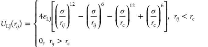
that is set to 180° for linear segments along backbone and side chains and to 90° at branching points. For nonbonded bead− bead interactions, we employed the standard shifted and truncated Lennard-Jones (LJ) potential

ε σ σ σ σ = − − + < > ⎧ ⎨ ⎪ ⎪ ⎩ ⎪ ⎪ ⎡ ⎣ ⎢ ⎢ ⎛ ⎝ ⎜⎜ ⎞ ⎠ ⎟⎟ ⎛ ⎝ ⎜⎜ ⎞ ⎠ ⎟⎟ ⎛_⎝⎜ ⎞ ⎠ ⎟ ⎛ ⎝ ⎜ ⎞ ⎠ ⎟ ⎤ ⎦ ⎥ ⎥ U r r r r r r r r r ( ) 4 , 0, ij ij ij ij ij LJ LJ 12 6 c 12 c 6 c c (3)

where rij is the distance between beads i and j. The implicit

solvent approach used in this study implies the absence of explicit interactions between polymer and solvent molecules. In this approach, hydrophobicity of ionomer groups in backbone and side chain units is embodied in the Lennard-Jones interaction parameter between apolar beads, εLJ, which must

be sufficiently attractive to adequately represent the so-called “poor-solvent” conditions.61,64,90−92

The cutoff distance was set to rc = 2.5 σ for interactions

between apolar polymer beads in the backbone and side chains. The value of εLJwas varied over the range specified inTable 1.

For all other pairs of beads (apolar−anionic, apolar−cationic, anionic−anionic, anionic−cationic), we used rc= 21/6σand εLJ

= 1 kBT. This treatment with a short cutoff distance for the

interactions involving charged beads and a longer cutoff for the interactions between apolar beads allows attractive and repulsive interactions to be adequately controlled and modulated.41−43,58,61,62,64,68,72,85,90−93 _{The value of ε}

LJ for

polymer−polymer interactions, simply referred to as εLJ

hereafter, was varied between 0.5 kBT and 1.5 kBT. The

baseline value εLJ = 1 kBT represents “normal hydrophobic”

behavior, while εLJ= 0.5 kBT and εLJ= 1.5 kBT correspond to

“weak” and “strong” hydrophobicity.90 The θ solvent conditions correspond to εLJ= 0.33 kBT.61,90

Charged beads interact via a direct Coulomb potential

λ = U r k T q q r ( )_ij B i j ij Coul B (4)

where λB= e02/4πε0εskBT is the Bjerrum length, e0is the unit

charge, and ε0 and εs are the permittivity of vacuum and the

relative dielectric constant of the solvent. The baseline value of the Bjerrum length is λB = 3.0 σ, which corresponds to

approximately 0.7 nm in aqueous electrolyte solution (σ = 0.25 nm).

Table 1 summarizes the baseline values and the range of variations of the model parameters εLJ, λB, Ns, and the

counterion valence Zc.

■

The particle−particle particle−mesh (PPPM)94 _{with an} accuracy of 10−5 was used for the calculation of electrostatic interactions. Simulations were carried out in the NVT ensemble with periodic boundary conditions in all three directions. A cubic box of side length L = 110 σ was chosen that is large enough to avoid finite size effects. The temperature was maintained through coupling of the system to a Langevin thermostat,95in which the motion of beads is described by

⃗ = −∇ ⃗ − Γ ⃗ + ⃗ m v t t U r t t F t d ( ) d d ( ) d ( ) i i i i i ₍₅₎

where Ui is the potential energy experienced by the ith bead

with mass mi, F⃗i(t) a random force with zero average value, and

Γ = τLJ−1a friction coefficient calibrated to maintain a reduced

temperature of T* = kBT/εLJ, where τLJis the standard LJ time,

τ_LJ= σ(m/εLJ)1/2. The classical Newtonian equations of motion

for beads were integrated using the velocity-Verlet algorithm with a time step of Δt = 0.01 τLJ. The time step in real units is

about 15 fs considering the choice of the length scale and the chemical mapping.

Simulations were performed with LAMMPS96 _{and VMD}97 was used for visualizations. The simulation protocol was as follows. A single stiff ionomer chain was placed in the middle of the simulation box and simulated for 2 × 106_{time steps. The}

chain was then replicated and distributed on a regular 3D grid in the simulation box. The system was run for 3 million time steps under fully repulsive short-range potential. This procedure resulted in random and homogeneous distribution of chains in the simulation box. Our ensemble of M = 25 chains corresponds to a number density of beads of ρ = MN/L3_{= 1.3}

×₁₀−3σ−3where N is the total number of beads in each chain. This density should be compared to the overlap monomer density of ρ* = N/(4/3πRg3), where Rgis the radius of gyration

for a single ionomer chain. Reference conditions of εLJ= 1 kBT

and λB = 3 σ result in ρ* = 1.2 × 10−2 σ−3. These values

indicate sufficiently dilute conditions with ρ = 0.1 ρ*. All simulations were run for 3.5 × 107 _{time steps,}

corresponding to 0.55 μs of total simulation time. The first 3.0 × 107 _{time steps were used for the equilibration that is}

tracked by monitoring the total energy of the system as well as the gyration radius of ionomer chains. For the equilibrium state Table 1. List of System Paramters and Their Baseline Values

along with the Explored Range

parameter baseline value parameter range explored in this work εLJ 1 kBT 0.5−1.5 kBT

λB 3.0 σ 1−12 σ

Ns 6 3−12

analysis, data collections were performed for the last 5 × 106

time steps, and data were saved every 1.0 × 105 _{time steps,}

resulting in 50 regularly spaced snapshots.

■

Calibrating the Backbone Flexibility.As a baseline, we aimed at simulating ionomer chains with the backbone fl_{exibility of Nafion-type ionomers. To this end, we determined}

kθby comparing the calculated persistence length, lp, of the bare

ionomer backbone (no side chains attached), simulated in the coarse-grained model, with reported values for a polytetra-fl_{uoroethylene (PTFE) chain.}9,98,99_{We calculated lpusing}93,100

∑

where b⃗j = r⃗j+1− r⃗j is the jth bond vector and b is the average

bond length, b ≈ 0.97 σ.Figure 2displays values of lp, obtained

in backbone simulations, as a function of kθ. Reported values for

the persistence length of Teflon are in the range of 2−5 nm.9,98,99_{We used the upper value of this range, l}

p = 5 nm,

which equals 20 σ in the coarse-grained ionomer model, to obtain an estimate of the corresponding kθ value. Figure 2

shows that kθ = 25 kBT produces the bending rigidity of a

semiflexible chain with lp= 20 σ. This value was employed for kθin all subsequent simulations.

Effect of Ionomer Hydrophobicity. Figure 3shows the impact of εLJ on ionomer aggregation. Starting from the

random initial dispersion of chains, shown in Figure 3a, cylindrical aggregates are formed at sufficiently large values of ε_LJ, while a more dispersed state prevails at low values of εLJ. In

aggregated structures, neutral backbone beads form the hydrophobic core region. Ionomer side chains and their anionic headgroups protrude out of the core region into the surrounding phase. Counterions form a diffuse halo around ionomer bundles. These bundle-like structures with cylindrical shape are in general agreement with cylindrical-like structures found in scattering studies of Nafion solutions.15,19−21,28,32

The aggregation number k, defined as the number of ionomer chains in a bundle, is calculated as the number of hydrophobic backbone beads in a single bundle divided by N. A bundle was identified as the group of monomers for which the smallest pairwise distance is less than the critical value, i.e., rij<

1.5 σ. Variation of this criterion between rij< 1.0 σ and rij< 2.5

σdid not alter the value of k. An average aggregation number ⟨k⟩ was calculated according to

∑

where M is the total number of ionomer chains in the box. In eq 7, P(ki) is the bundle size distribution function defined as

P(ki) = ⟨N(ki)⟩/∑i=1M⟨N(ki)⟩, where N(ki) is the number of ki

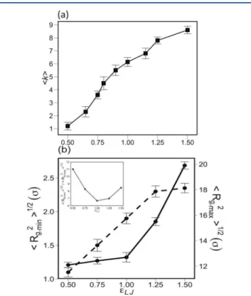
bundles and ⟨...⟩ denotes the time averaging over equilibrium trajectories.Figure 4a shows the variation of ⟨k⟩ as a function of ε_LJ. The dependence of ⟨k⟩ on εLJis monotonic. The growth in

bundle size observed upon increasing εLJ is consistent with a

theory of ionomer aggregation presented in ref80.

Figure 2. Calculated persistence length of single linear chain mimicking the ionomer backbone. A value of kθ= 25 kBT reproduces the persistence length of a PTFE chain. The snapshots show typical chain conformations in different regimes of chain rigidity. All the error bars in this article represent the standard deviations obtained over the equilibrium trajectories.

Figure 3.(a) Initial configuration of chains in the simulation box; (b) to (d) show snapshot of the self-assembled structure at different values of εLJ= 0.5, 1.0, and 1.5 kBT. The color coding is the same as inFigure

2. A close-up of a typical bundle is shown below the εLJ= 1.0 kBT box.

Figure 4.(a) Change in average aggregate size, ⟨k⟩, as a function of the interaction parameter εLJbetween apolar beads. (b) Change in the minimum (radial) and maximum (longitudinal) bundle size vs εLJ. The inset shows the aspect ratio of ionomer bundles.

At low values, εLJ ≤ 0.75 kBT, representing weak

hydro-phobicity of backbone chains, the increase in free energy upon bundle formation due to the loss in chain entropy outweighs the decrease in potential energy due to the aggregation of backbones; therefore, in this regime, ionomer chains remain in a dispersed state with bundle sizes of ⟨k⟩ ≈ 1−2. In the regime of large εLJ > 1 kBT, the energy loss upon aggregation of

hydrophobic backbones becomes the dominant contribution to the free energy, outweighing the impact of the entropy loss and of the increase in the electrostatic interaction energy between anionic beads at the bundle surface; therefore in this regime, the equilibrium bundle size shifts to larger values.

The shape and dimension of ionomer bundles were obtained from the radius of gyration tensor (S) of each aggregate. For every aggregate a gyration tensor is constructed that is then diagonalized to calculate the three eigenvalues, λ1, λ2, and λ3.

The squared gyration radius of bundles, Rg2, would be the first

invariant of S, Tr S = λ1+ λ2+ λ3, while the second invariant

gives the relative shape anisotropy defined as κ2_{= (3S − Tr S·} E)/2(Tr S)2with E being the unit tensor;101−104_κ2_{ranges from}

0 for a sphere (λ1 = λ2= λ3) to 1/4 for a planar symmetric

object (λ1= λ2, λ3= 0) and to 1 for a rod (λ2= λ3= 0). These

eigenvalues are averaged over the ensemble of ionomer bundles in the simulation box. The imposed bending rigidity yields cylindrical (λ1 > λ2 ≈ λ3) ionomer bundles. The largest

eigenvalue, denoted as ⟨Rg,max2⟩1/2, corresponds to the average

length of an ionomer bundle, while the average of the remaining two λ values, denoted as ⟨Rg,min2⟩1/2, corresponds

to the bundle thickness. Figure 4b shows ⟨Rg,max2⟩1/2 and

⟨Rg,min2⟩1/2 as functions of εLJ; the inset depicts the bundle

aspect ratio ⟨Rg,max2⟩1/2/⟨Rg,min2⟩1/2. In the range εLJ < 1 kBT,

bundles grow mainly in radial direction upon increasing εLJ. At

ε_LJ> 1 kBT, a pronounced growth trend in bundle length sets

in. The plot of the aspect ratio shows a minimum at εLJ= 1 kBT.

Isolation of anionic headgroups from the surrounding counter-ions upon further radial bundle growth would cause desolvation of anionic headgroups, causing a sudden increase in the bundle free energy.64,65 _{This energetically unfavorable process that} depends on the length of side chains prevents the further radial growth of bundles. It is responsible for the preferential longitudinal growth at εLJ> 1 kBT.

Detailed analyses of bundle structures involve the calculation of radial distribution functions (RDFs) of interacting beads,

g(r). For an isotropic system, an RDF gA−B(r) describes the

probability of finding a particle A in a specific radial distance, r, of a reference particle B. It is defined as105

∑ ∑

where NAand NBare the numbers of A and B particles in the

simulated system, respectively. The triangle brackets around the δ-function indicate averaging over the equilibrium system trajectory. RDF plots presented in the following are normalized to the volume per bundle and to the number of beads of type A or B per bundle.

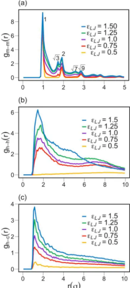
Figure 5 shows the RDFs of apolar backbone monomers,

g_m−m(r), anionic headgroups, gh−h(r), and between headgroups

and counterions, gh−c(r), at different values of εLJ. Figure 5a

shows the increase in gm−m(r) with increasing εLJ. This trend

exhibits the enhanced aggregation of ionomer backbones as the result of an increased segregation strength. The plot furthermore reveals a dense hexagonal packing of ionomer

chains in the bundle core, indicated by the ratio of peak separations in gm−m(r) that follows a sequence 1:√3:2:√7:√9,

as indicated in the plot. This hexagonal form of packing was also found in refs 17 and 19−22 for self-assembled Nafion chains in dilute solution as well as for self-assembled polyelectrolyte chains.25

The aggregation of backbone chains with pendant charged side chains results in the formation of ion-rich regions in solution, as can be observed in the RDFs gh−h(r) and gh−c(r),

shown inFigures 5b and 5c. There is no specific correlation among headgroups in the regime of weak hydrophobicity, εLJ=

0.5 kBT. However, gh−h(r) grows as εLJ increases, and two

correlation peaks emerge. Increasing εLJenhances the intensity

of gh−h(r) due to the presence of a greater number of backbone

chains in the bundle, which results in a greater total number of anionic headgroups at the bundle surface. The locations of the fi_{rst and second peak are not altered for εLJ= 0.75 kBT, 1 kBT,} and 1.25 kBT. However, these peaks are shifted to smaller

values, indicating a densification of surface groups, in the case of strong hydrophobicity, i.e., for εLJ= 1.5 kBT.

The RDF gh−c(r), depicted inFigure 5c for various values of

ε_LJ, reveals that the counterion localization in the vicinity of headgroups increases with εLJ. A higher charge density and a

greater surface potential in bundles with stronger hydrophobic interactions induces stronger electrostatic attraction on counterions. This stronger interaction results in a greater localization of counterions around bundles. Further inspection

Figure 5.Radial distribution functions of (a) monomer−monomer, gm−m(r), (b) headgroup−headgroup, gh−h(r), and (c) headgroup− counterion, gh−c(r), at different values of εLJ. Peak location ratios are shown in (a) by considering the first peak as the reference peak.

ofFigure 3affirms the formation of a counterion cloud at the bundle surface in the regime of strong hydrophobicity.

Effect of Electrostatic Interaction Strength. In this section, we explore the changes in aggregation behavior upon variation of λB, while fixing εLJ= 1 kBT. The change of λBin

experiment can be achieved through variation of the dielectric constant of the solvent. In all simulations performed with varying values of λBthe formation of cylindrical bundles was

observed.

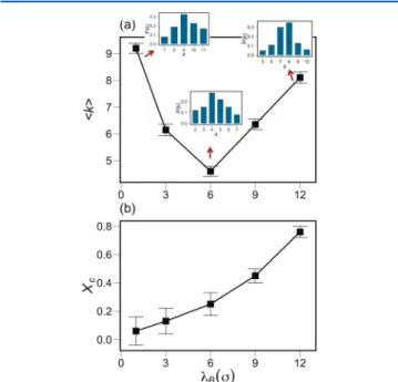
The nonmonotonic behavior in the plot of ⟨k⟩ vs λB in

Figure 6a can be explained as follows: the decreasing trend for

λ_B < 6 σ is caused by the electrostatic repulsion of anionic charges on the bundle surface that disfavors aggregation; however, at large values of λB, for λB> 6 σ, the trend is reversed

due to the effect of counterion localization shown inFigure 6b. The fraction of localized counterions, Xc, is defined as the

number of counterions in radial distance <2.5 σ of the nearest headgroup.67,78_X

c is an increasing function of λB. Counterion

localization results in an effective screening of the anionic charges and a correspondingly reduced effective Coulomb repulsions between headgroups.

For λB< 6 σ, the majority of counterions remain dispersed

(nonlocalized) in the electrolyte. In this regime of weak counterion localization, the free energy change upon increasing λ_B is mainly determined by the increasing electrostatic repulsion between anionic headgroups. This dependence disfavors aggregation, which is responsible for the decrease in ⟨k⟩ with λB and the evolution of a more dispersed ionomer

solution, as shown by the changes in the size distribution functions shifting from λBvalues of 1 σ to 6 σ.

At λB > 6 σ, the effect of counterion localization

overcompensates the increase in the direct Coulomb interaction between headgroups, leading to a net decrease in the effective electrostatic energy with increasing λBand growing

⟨k⟩, and formation of a phase-separated ionomer solution. A

nonmonotonic dependence on Bjerrum length was also

observed in refs67 and 78 for the variation in the thickness of polyelectrolyte brushes.

Figure 7 shows the RDF of backbone monomers for the range of explored λB values. gm−m(r) demonstrates a

non-monotonic dependence on λB. The spatial ordering of the

ionomer chains in the bundle core is retained for the explored values of the Bjerrum length. Ionomer bundles with the smallest λB(λB= 1 σ) exhibit the largest magnitude of peaks in g_m−m(r). The RDF gm−m(r) decreases as λB increases to 6 σ.

Further increase in λB above 6 σ results in an upsurge in g_m−m(r). These trends are consistent with the trends in the bundle size reported inFigure 6a.

Effect of Side Chain Density. The effect of the side chain density on the aggregation behavior of ionomer chains is studied by increasing the number of grafting sites, Ns, at fixed

length of the ionomer backbone.Figure 8shows the solution of

ionomer aggregates for Ns = 3, 6, 9, 15 with fixed εLJ= 1 kBT

and λB= 3 σ. Increasing Nsis accompanied by the formation of

a larger number of aggregates with smaller sizes.

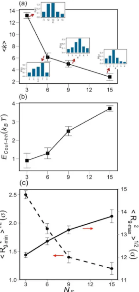
Figure 9a shows the dependence of the bundle size on Ns.

Larger Ns results in shorter distance among the anionic

headgroups. The decrease in ⟨k⟩ with increasing Ns, seen in

Figure 9a, can be attributed to the enhanced electrostatic repulsion between anionic headgroups that increases the bundle free energy and disfavors aggregation. The size distribution functions also clearly show the shift of the ionomer ensemble from a phase-separated system of large aggregates to a system consisting of small ionomer bundles.

Figure 9b shows the increase of the Coulomb interaction energy of headgroups (per headgroup) as a function of Ns. This

interaction energy is obtained by isolating the electrostatic and short-range portions of the mutual headgroup interactions.

Figure 9c shows the change in the longitudinal and radial bundle dimension as a function of Ns. The decrease in the

Figure 6.(a) Dependence of average bundle size on the value of λB. Imbedded plots show the distribution function of the bundle number vs k for λB= 1 σ, 6 σ, and 12 σ; (b) shows the fraction of counterions within 2.5 σ of the anionic headgroups.

Figure 7.Monomer−monomer RDF gm−m(r) for different values of the Bjerrum length.

Figure 8.Snapshots showing the ionomer bundles at different values of Ns: (a) Ns= 3, (b) Ns= 6, (c) Ns= 9, (d) Ns= 15.

⟨R_g,min2_⟩1/2 _{follows the same trend as ⟨k⟩. An increase in}

⟨Rg,max2⟩1/2, in the range 2 σ, occurs upon increasing Nsfrom 3

to 15. This range of variation in the bundle length mostly originates from the Coulombic-induced chain stretching upon increasing the number of pendant ionic side chains.

Figure 10displays the RDFs among headgroup units for the fi_{nal aggregated structures at different N}

s. Bundles formed from

chains with smaller Nsare more populated of headgroups than

the bundles formed from chains with greater Ns values. The

observed trend in gh−h(r) is attributed to the larger bundles that

form from ionomer chains with fewer side chains.

The side chain content in commercial PFSAs such as 3M, Hyflon, and Nafion is primarily expressed in terms of the ion exchange capacity (IEC) of the polymer membrane, defined as the number of moles of acid groups over the mass of dry membrane. Major dissimilarity in PFSA ionomers with different side chain chemistries is manifested in terms of their different side chain contents. The side chain lengths of ionomer materials such as 3M, Hyflon, and Nafion vary in the range from 5.27 to 8.44 Å.81 We simulated systems with ls varying

from 1 σ to 6 σ. We did not find any clearly discernible trend in bundle size as a function of ls. The length of side chains has

however a strong impact on the dynamics of individual ionomer chains; therefore, over the simulation time of 3.5 × 107_time

steps, no equilibration was observed for ionomer systems with ls

= 6 σ. We will discuss the impact of the side chain length on ionomer properties in a forthcoming publication.

Effect of Counterion Valence. The effect of the counterion valence on the aggregation behavior of ionomer chains was investigated by comparing results for Zc = +1, +2,

and +3. Figure 11depicts the final snapshots for the systems

with different counterion valences. As Zcincreases, the solution

contains fewer but larger ionomer bundles. In the case of trivalent counterions, we can see the formation of a weakly bent and elongated worm-like bundle. The localization of counter-ions in the vicinity of ionomer bundles increases dramatically with Zc because of the stronger electrostatic attraction of

multivalent counterions to the anionic headgroups. This trend is clearly observed in Figure 11 where almost all the counterions are strongly localized near the anionic headgroups for Zc= +3.

The enhanced localization results in screening the repulsion of anionic headgroups, thereby enabling the growth of larger bundles. Strong localization of multivalent counterions also induces an attractive interaction106among charged units known as the bridging107effect. Figure 12a shows that ⟨k⟩ increases significantly with Zc. Figure 12b shows that the fraction of

strongly localized counterions (within 2.5 σ), Xc, increases

monotonously with Zc.Figure 12c reveals a 2-fold increase in

average bundle length and an increase by 0.8 σ in the bundle thickness with Zc. This observation points out the preferential

longitudinal assembly and growth of ionomer bundles upon increase in Zc.

It is interesting to analyze the influence of counterion valence on the dynamics of backbone monomers and counterions by calculating the mean-square displacement (MSD) of these species. The MSD is calculated according to

= ⟨| − | ⟩

t r t r

MSD( ) _i( ) _i(0)2 (9)

after subtracting the center of mass of the corresponding beads. Figure 13 shows the MSD of counterions and backbone monomer beads during the simulation for different Zc.Figure

Figure 9. Effect of Ns on (a) equilibrium aggregate size, ⟨k⟩ (imbedded plots show the distribution function of the bundle number vs k), (b) Coulombic energy of anionic headgroups, and (c) maximum and minimum bundle gyration radius.

Figure 10. Radial distribution function among anionic headgroups, gh−h(r), for the explored values of Ns.

Figure 11. Morphologies of ionomer solutions for solutions containing (a) monovalent, Zc= +1, (b) divalent, Zc= +2, and (c) trivalent, Zc= +3, counterions.

13a reveals that the strong localization of counterions for Zc=

+3 markedly diminishes their mobility. The backbone dynamics is also slowed down with increased Zc because of the larger

number of chains in the bundle core and the increased number of monomer−monomer contacts. Yan et al.69also observed the decrease in the counterion dynamics upon increasing its valency due to stronger bonding to the polyelectrolyte.

■

We have systematically explored the impact of primary parameters of the ionomer−solvent system on the aggregation behavior of ionomer molecules in dilute solution. Here, we will reiterate the main trends and evaluate them in comparison to experimental findings reported in the literature.

Simulation results suggest that aggregation numbers of PFSA-type ionomers can be expected to lie in the range of ⟨k⟩ = 6−10, as seen inFigures 4,6a,9a, and12a for our reference set of parameters. This range is consistent with stable aggregate sizes of k = 9 that the theory of ionomer aggregation presented in ref 80 predicted for a set of baseline parameters that corresponds to PFSA ionomers in aqueous solution.

Increased hydrophobicity resulted in the formation of larger bundles. A change in the strength of the hydrophobic interactions between apolar polymer beads, represented in the model by the parameter εLJ, can be induced through

alteration of the ionomer chemistry, for instance, by replacing fl_{uorocarbon with hydrocarbon chains. Less hydrophobic} hydrocarbon ionomers exhibit smaller values of εLJ that

diminish the tendency for bundle formation, resulting in more dispersed solution characteristics. Comparative exper-imental investigation of the solution features of hydrocarbon and PFSA ionomers would be highly insightful in this regard.

The second major parametric effect refers to the grafting density of side chains. In the model study it is evaluated by varying the number Ns of side chains per ionomer backbone

chain (with fixed length). We observed in Figure 9a that an increase in Ns results in a monotonic decrease in bundle size,

leading to a dispersed ionomer state in the limit of high Ns. The

ionic content of ionomers is controlled during the synthesis process. Experimental studies of Loppinet and Gebel19confirm the decrease in bundle size in solutions of PFSA-type ionomers with higher side chain content. A similar decreasing trend in aggregation behavior was seen in SAXS studies by Rulkens et al.25 performed on solutions of semirigid poly(p-phenylene)s (PPP) chains upon increasing the sulfonate ion content. In the limit of very high ionic content such systems assumed the configuration of nonaggregating and dispersed polyelectrolyte chains.

A way to isolate the impact of direct Coulomb interactions on ionomer aggregation is to add salt ions to the solution that screen the electric charges and reduce the value of λB. Jiang et

al.21studied the size of Nafion bundles in solution at different salt contents. Increasing the salt concentration resulted in an increase in the size of Nafion bundles, consistent with the trend seen in Figure 6a at low λB. Experimental studies exploring

regimes of strong electrostatic interactions are needed to capture the predicted nonmonotonic dependence of the bundle size on the strength of electrostatic interactions.

Employing solvents with different dielectric properties exerts a more complex impact on the aggregation behavior. In simulations, changes in solvent properties affect the interplay between solvent-mediated interactions of apolar ionomer groups, embodied in the simulation parameter εLJ, and direct

Figure 12.Effect of counterion valence Zcon (a) average bundle sizes, (b) fraction of localized counterions, and (c) effective length and diameter of bundles.

Figure 13.(a) MSD of counterions with different valences and (b) changes in MSD of backbone monomer beads for bundles formed in the presence of counterion with different valence Zc.

Coulomb interactions, embodied in the Bjerrum length, λB. A

less polar solvent will decrease the value of εLJ for the

hydrophobic ionomer, thus disfavoring the aggregation of backbones, and increase the value of λB, representing an

increase in the strength of direct Coulomb interactions. Looking atFigure 6a, we should distinguish two regimes. In the regime of small λB, i.e., λB< 6 σ, Coulomb interactions of

anionic headgroups are weakly screened by diffuse counterions. In this regime of weak counterion localization, the less polar solvent causes consistent trends in aggregation behavior exerted by εLJand λB: the net effect is a decrease in ⟨k⟩ for the less polar

solvent. In the regime of high λB, i.e. λB> 6 σ, the screening

effect due to strong counterion localization in the vicinity of bundles comes into play, reverting the impact of solvent polarity on effective electrostatic interactions. In this regime of strong counterion localization, the impacts of variations in εLJ

and λB on ionomer aggregation oppose each other: the less

polar solvent tends to weaken aggregation via εLJand enhance

aggregation via λB; a general trend of the net effect cannot be

predicted.

Loppinet et al.19,20observed, using SAXS and SANS, that the radius of rod-like Nafion aggregates increased when more polar solvents that are solvents with higher dielectric constant and greater εLJ were employed. They observed a shift in the

ionomer peak to lower q values for aqueous solvents compared to alcoholic solvents (with λb≈ 9 σ by considering ε ≈ 25),

indicating larger radius of ionomer aggregates in solvents with higher polarity. Consistently, a decrease in aggregate size of Nafion ionomer was seen by Welch et al.108when water was replaced with glycerol, a less polar solvent. These trends are in accord with the trends predicted by simulations in the regime of weak counterion localization.

Experimentally, there is no direct study regarding the influence of counterion valency on the colloidal aggregation of hydrophobic ionomer chains or PFSA chains in dilute solution. On the membrane level, counterion valence was seen to have a strong impact on the mechanical properties of the ionomer membrane.45,109_{These changes can possibly originate} from the fundamental structural reorganization at the bundle level. However, trying to relate these membrane studies to our solution-based simulations would be speculative at this point.

■

In this study, we have applied coarse-grained molecular dynamics simulations to study the aggregation of ionomer chains in dilute solution with no added electrolyte. Simulations account for the short-range interactions of apolar hydrophobic polymer groups in ionomer backbone and side chains as well as explicit Coulomb indications between charged moieties, viz. anionic headgroups and counterions in solution. The interplay of these interactions controls the formation of ionomer aggregates or bundles of finite size. Stable bundles attain a cylindrical-like shape with dense hexagonal packing arrange-ment of ionomer backbones. The size of stable bundles, the density of anionic headgroups at their surface, and the distribution of counterions in the surrounding solution depend on the primary ionomer chemistry and architecture, viz., the chemical nature of polymer groups, the grafting density of side chains, and the properties of the solvent. We found that a stronger backbone hydrophobicity of polymer groups results in larger bundle sizes. Increasing the grafting density of acid-terminated side chains leads to a monotonic decrease in bundle size. A variation in the strength of Coulomb interactions gives

rise to a nonmonotonic trend in bundle size: in a regime of weak counterion localization, corresponding to a small Coulomb interaction parameter, bundle size decreases with increasing interaction strength; in a regime of strong counter-ion localizatcounter-ion, attained for large Coulomb interactcounter-ion parameter, the bundle size increases with increasing interaction strength. Ionomers with higher number of pendant groups form smaller bundles due to stronger electrostatic repulsion among their anionic moieties. Increasing the valence of counterions from one to three results in a pronounced increase in bundle size, and more strikingly it leads to an almost complete depletion of the solution from counterions owed to pronounced counterion condensation at the bundle surface. This effect is expected to have a strong impact on ion transport phenomena in the membrane. Generally, trends predicted based on our computational study are consistent with experimental observations. The ability to correlate primary ionomer parameters and solvent properties with the structure and electrostatic properties of ionomer bundles is crucial for a rational design of membrane-forming materials. In related work, we study how the mechanical and electrostatic properties of microscopic bundles determine water sorption and swelling, transport phenomena, chemical degradation, and mechanical failure of ionomer-based membranes. The present work is a vital step toward a basic understanding on how to modify ionomer and solvent properties in order to obtain polymer electrolyte membranes with improved performance and stability.

■

Corresponding Author

*_{E-mail: meikerl@sfu.ca(M.H.E.).}

Notes

The authors declare no competing financial interest.

■

The work reported in this manuscript was performed with the fi_{nancial support from an NSERC Discovery Grant, entitled}

Materials for Electrochemical Energy Conversion: From Funda-mental Physics to Advanced Design. Simulations were performed

using the Grex computational facility at the University of Manitoba, provided through WestGrid and Compute Canada.

■

(1) Nomula, S.; Cooper, S. L. Macromolecules 2001, 34, 2653−2659. (2) Nomula, S.; Cooper, S. L. J. Phys. Chem. B 2000, 104, 6963− 6972.

(3) Schlick, S. Ionomers: Characterization, Theory, and Applications; CRC Press: Boca Raton, FL, 1996.

(4) Eisenberg, A.; Kim, J.-S. Introduction to Ionomers; John Wiley & Sons: New York, 1998.

(5) Zhang, L.; Brostowitz, N. R.; Cavicchi, K. A.; Weiss, R. A. Macromol. React. Eng. 2014, 8, 81−99.

(6) Eikerling, M.; Kulikovsky, A. Polymer Electrolyte Fuel Cells: Physical Principles of Materials and Operation; CRC Press: Boca Raton, FL, 2014.

(7) Grot, W. G. Macromol. Symp. 1994, 82, 161−172.

(8) Eikerling, M.; Paddison, S. J.; Zawodzinski, T. A. J. New Mater. Electrochem. Syst. 2002, 5, 15−23.

(9) Schmidt-Rohr, K.; Chen, Q. Nat. Mater. 2008, 7, 75−83. (10) Mauritz, K. A.; Moore, R. B. Chem. Rev. 2004, 104, 4535−4585. (11) Gierke, T. D. .; Munn, G. E. .; Wilson, F. C. J. Polym. Sci., Polym. Phys. Ed. 1981, 19, 1687−1704.

(13) Haubold, H. G.; Vad, T.; Jungbluth, H.; Hiller, P. Electrochim. Acta 2001, 46, 1559−1563.

(14) Berrod, Q.; Lyonnard, S.; Guillermo, A.; Ollivier, J.; Frick, B.; Manseri, A.; Améduri, B.; Gébel, G. Macromolecules 2015, 48, 6166− 6176.

(15) Rubatat, L.; Rollet, A. L.; Gebel, G.; Diat, O. Macromolecules 2002, 35, 4050−4055.

(16) Rubatat, L.; Gebel, G.; Diat, O. Macromolecules 2004, 37, 7772− 7783.

(17) Aldebert, P.; Dreyfus, B.; Pineri, M. Macromolecules 1986, 19, 2651−2653.

(18) Rollet, A. L.; Gebel, G.; Simonin, J. P.; Turq, P. J. Polym. Sci., Part B: Polym. Phys. 2001, 39, 548−558.

(19) Loppinet, B.; Gebel, G. Langmuir 1998, 14, 1977−1983. (20) Loppinet, B.; Gebel, G.; Williams, C. E. J. Phys. Chem. B 1997, 101, 1884−1892.

(21) Jiang, S.; Xia, K.-Q.; Xu, G. Macromolecules 2001, 34, 7783− 7788.

(22) Aldebert, P.; Dreyfus, B.; Gebel, G.; Nakamura, N.; Pineri, M.; Volino, F. J. Phys. (Paris) 1988, 49, 2101−2109.

(23) Szajdzinska-Pietek, E.; Schlick, S.; Plonka, A. Langmuir 1994, 10, 1101−1109.

(24) Szajdzinska-Pietek, E.; Schlick, S.; Plonka, A. Langmuir 1994, 10, 2188−2196.

(25) Rulkens, R.; Wegner, G.; Thurn-Albrecht, T. Langmuir 1999, 15, 4022−4025.

(26) Kroeger, A.; Deimede, V.; Belack, J.; Lieberwirth, I.; Fytas, G.; Wegner, G. Macromolecules 2007, 40, 105−115.

(27) Zaroslov, Y. D.; Gordeliy, V. I.; Kuklin, A. I.; Islamov, A. H.; Philippova, O. E.; Khokhlov, A. R.; Wegner, G. Macromolecules 2002, 35, 4466−4471.

(28) Gebel, G.; Loppinet, B.; Hara, H.; Hirasawa, E. J. Phys. Chem. B 1997, 101, 3980−3987.

(29) Rubatat, L.; Diat, O. Macromolecules 2007, 40, 9455−9462. (30) Lin, H. L.; Yu, T. L.; Huang, C. H.; Lin, T. L. J. Polym. Sci., Part B: Polym. Phys. 2005, 43, 3044−3057.

(31) He, L.; Fujimoto, C. H.; Cornelius, C. J.; Perahia, D. Macromolecules 2009, 42, 7084−7090.

(32) Paul, D. K.; Karan, K.; Docoslis, A.; Giorgi, J. B.; Pearce, J. Macromolecules 2013, 46, 3461−3475.

(33) Malek, K.; Eikerling, M.; Wang, Q.; Navessin, T.; Liu, Z. J. Phys. Chem. C 2007, 111, 13627−13634.

(34) Yamaguchi, M.; Matsunaga, T.; Amemiya, K.; Ohira, A.; Hasegawa, N.; Shinohara, K.; Ando, M.; Yoshida, T. J. Phys. Chem. B 2014, 118, 14922−14928.

(35) Eikerling, M. H.; Berg, P. Soft Matter 2011, 7, 5976−5990. (36) Eikerling, M.; Kornyshev, A. A.; Kuznetsov, A. M.; Ulstrup, J.; Walbran, S. J. Phys. Chem. B 2001, 105, 3646−3662.

(37) Eikerling, M.; Kornyshev, A. A.; Spohr, E. In Fuel Cells I; Springer: Berlin, 2008; Vol. 215, pp 15−54.

(38) Vartak, S.; Roudgar, A.; Golovnev, A.; Eikerling, M. J. Phys. Chem. B 2013, 117, 583−588.

(39) Ghelichi, M.; Melchy, P.-É. A.; Eikerling, M. H. J. Phys. Chem. B 2014, 118, 11375−11386.

(40) Rodgers, M. P.; Bonville, L. J.; Kunz, H. R.; Slattery, D. K.; Fenton, J. M. Chem. Rev. 2012, 112, 6075−6103.

(41) Hall, L. M.; Seitz, M. E.; Winey, K. I.; Opper, K. L.; Wagener, K. B.; Stevens, M. J.; Frischknecht, A. L. J. Am. Chem. Soc. 2012, 134, 574−587.

(42) Hall, L. M.; Stevens, M. J.; Frischknecht, A. L. Macromolecules 2012, 45, 8097−8108.

(43) Goswami, M.; Kumar, S. K.; Bhattacharya, A.; Douglas, J. F. Macromolecules 2007, 40, 4113−4118.

(44) Cui, S.; Liu, J.; Selvan, M. E.; Keffer, D. J.; Edwards, B. J.; Steele, W. V. J. Phys. Chem. B 2007, 111, 2208−2218.

(45) Daly, K. B.; Panagiotopoulos, A. Z.; Debenedetti, P. G.; Benziger, J. B. J. Phys. Chem. B 2014, 118, 13981−13991.

(46) Knox, C. K.; Voth, G. A. J. Phys. Chem. B 2010, 114, 3205− 3218.

(47) Lucid, J.; Meloni, S.; Mackernan, D.; Spohr, E.; Ciccotti, G. J. Phys. Chem. C 2013, 117, 774−782.

(48) Urata, S.; Irisawa, J.; Takada, A.; Shinoda, W.; Tsuzuki, S.; Mikami, M. J. Phys. Chem. B 2005, 109, 4269−4278.

(49) Jang, S. S.; Molinero, V.; Cagin, T.; Goddard, W. A., III J. Phys. Chem. B 2004, 108, 3149−3157.

(50) Vishnyakov, A.; Neimark, A. V. J. Phys. Chem. B 2014, 118, 11353−11364.

(51) Hristov, I. H.; Paddison, S. J.; Paul, R. J. Phys. Chem. B 2008, 112, 2937−2949.

(52) Wang, C.; Paddison, S. J. Soft Matter 2014, 10, 819−830. (53) Yamamoto, S.; Hyodo, S.-A. Polym. J. 2003, 35, 519−527. (54) Vishnyakov, A.; Neimark, A. V. J. Phys. Chem. B 2001, 105, 9586−9594.

(55) Malek, K.; Eikerling, M.; Wang, Q.; Liu, Z.; Otsuka, S.; Akizuki, K.; Abe, M. J. Chem. Phys. 2008, 129, 204702−204710.

(56) Komarov, P. V.; Veselov, I. N.; Chu, P. P.; Khalatur, P. G. Soft Matter 2010, 6, 3939−3956.

(57) Adamcik, J.; Mezzenga, R. Macromolecules 2012, 45, 1137− 1150.

(58) Karatasos, K. Macromolecules 2008, 41, 1025−1033.

(59) Srinivas, G.; Shelley, J. C.; Nielsen, S. O.; Discher, D. E.; Klein, M. L. J. Phys. Chem. B 2004, 108, 8153−8160.

(60) Wang, S.; Larson, R. G. Langmuir 2015, 31, 1262−1271. (61) Grest, G. S.; Murat, M. Macromolecules 1993, 26, 3108−3117. (62) Hall, L. M.; Stevens, M. J.; Frischknecht, A. L. Phys. Rev. Lett. 2011, 106, 1−4.

(63) Khalatur, P. G.; Khokhlov, A. R.; Mologin, D. A.; Reineker, P. J. Chem. Phys. 2003, 119, 1232−1247.

(64) Limbach, H. J.; Holm, C.; Kremer, K. Macromol. Chem. Phys. 2005, 206, 77−82.

(65) Limbach, H. J.; Sayar, M.; Holm, C. J. Phys.: Condens. Matter 2004, 16, S2135−S2144.

(66) Omar, A. K.; Hanson, B.; Haws, R. T.; Hu, Z.; Bout, D. A.; Vanden; Rossky, P. J.; Ganesan, V. J. Phys. Chem. B 2015, 119, 330− 337.

(67) Sandberg, D. J.; Carrillo, J. M. Y.; Dobrynin, A. V. Langmuir 2009, 25, 13158−13168.

(68) Stevens, M. J. Phys. Rev. Lett. 1999, 82, 101−104. (69) Yan, L.-T.; Guo, R. Soft Matter 2012, 8, 660.

(70) Wong, G. C.; Tang, J. X.; Lin, A.; Li, Y.; Janmey, P. A.; Safinya, C. R. Science 2000, 288, 2035−2039.

(71) Tang, J. X.; Janmey, P. A. J. Biol. Chem. 1996, 271, 8556−8563. (72) Vasilevskaya, V. V.; Markov, V. A.; Ten Brinke, G.; Khokhlov, A. R. Macromolecules 2008, 41, 7722−7728.

(73) Morriss-Andrews, A.; Shea, J. E. J. Phys. Chem. Lett. 2014, 5, 1899−1908.

(74) Mohammadinejad, S.; Fazli, H.; Golestanian, R. Soft Matter 2009, 5, 1522−1529.

(75) Goobes, R.; Cohen, O.; Minsky, A. Nucleic Acids Res. 2002, 30, 2154−2161.

(76) Rogers, P. H.; Michel, E.; Bauer, C. A.; Vanderet, S.; Hansen, D.; Roberts, B. K.; Calvez, A.; Crews, J. B.; Lau, K. O.; Wood, A.; Pine, D. J.; Schwartz, P. V. Langmuir 2005, 21, 5562−5569.

(77) Fu, I. W.; Markegard, C. B.; Chu, B. K.; Nguyen, H. D. Langmuir 2014, 30, 7745−7754.

(78) Carrillo, J. M. Y.; Dobrynin, A. V. Langmuir 2009, 25, 13158− 13168.

(79) Hess, B.; Sayar, M.; Holm, C. Macromolecules 2007, 40, 1703− 1707.

(80) Melchy, P. É. A.; Eikerling, M. H. Phys. Rev. E 2014, 89, 032603−032609.

(81) Clark, J. K.; Paddison, S. J. J. Phys. Chem. A 2013, 117, 10534− 10543.

(82) Choi, P.; Jalani, N. H.; Datta, R. J. Electrochem. Soc. 2005, 115, E123−E130.

(83) Zhang, C.; Knyazev, D. G.; Vereshaga, Y. A.; Ippoliti, E.; Nguyen, T. H.; Carloni, P.; Pohl, P. Proc. Natl. Acad. Sci. U. S. A. 2012, 109, 9744−9749.

(84) Marcus, Y. J. Chem. Phys. 2012, 137, 154501.

(85) Kremer, K.; Grest, G. S. J. Chem. Phys. 1990, 92, 5057−5086. (86) Binder, K. Monte Carlo and Molecular Dynamics Simulations in Polymer Science; Oxford University Press: New York, 1995.

(87) Kotelyanskii, M.; Theodorou, D. N. Simulation Methods for Polymers; CRC Press: Boca Raton, FL, 2004.

(88) Dunweg, B.; Kremer, K. J. Chem. Phys. 1993, 99, 6983−6997. (89) Binder, K. Monte Carlo and Molecular Dynamics Simulations in Polymer Science; Oxford University Press: New York, 1995.

(90) Micka, U.; Holm, C.; Kremer, K. Langmuir 1999, 15, 4033− 4044.

(91) Carrillo, J.-M. Y.; Dobrynin, A. V. Macromolecules 2011, 44, 5798−5816.

(92) Košovan, P.; Limpouchová, Z.; Procházka, K. J. Phys. Chem. B 2007, 111, 8605−8611.

(93) Stevens, M. J.; Kremer, K. J. Chem. Phys. 1995, 103, 1669−1690. (94) Darden, T.; York, D.; Pedersen, L. J. Chem. Phys. 1993, 98, 10089−10092.

(95) Grest, G. S.; Kremer, K. Phys. Rev. A: At., Mol., Opt. Phys. 1986, 33, 3628−3631.

(96) Plimpton, S. J. Comput. Phys. 1995, 117, 1−19,http://lammps. sandia.gov,.

(97) Humphrey, W.; Dalke, A.; Schulten, K. J. Mol. Graphics 1996, 14, 33−38,http://www.ks.uiuc.edu/Research/vmd/,.

(98) Rosi-Schwartz, B.; Mitchell, G. R. Polymer 1996, 37, 1857− 1870.

(99) Chu, B.; Wu, C.; Bucks, W. Macromolecules 1989, 22, 831−837. (100) Ullner, M.; Jönsson, B.; Peterson, C.; Sommelius, O.; Söderberg, B. J. Chem. Phys. 1997, 107, 1279−1287.

(101) Šolc, K. J. Chem. Phys. 1971, 55, 335−344.

(102) Theodorou, D. N.; Suter, U. W. Macromolecules 1985, 18, 1206−1214.

(103) Arkin, H.; Janke, W. J. Chem. Phys. 2013, 138, 054904. (104) Šolc, K.; Stockmayer, W. H. J. Chem. Phys. 1971, 54, 2756− 2757.

(105) Allen, M. P.; Tildesley, D. J. Computer Simulation of Liquids; Clarendon Press: New York, 1989.

(106) Dobrynin, A. V. Macromolecules 2006, 39, 9519−9527. (107) Liu, S.; Ghosh, K.; Muthukumar, M. J. Chem. Phys. 2003, 119, 1813−1823.

(108) Welch, C.; Labouriau, A.; Hjelm, R.; Orler, B.; Johnston, C.; Kim, Y. S. ACS Macro Lett. 2012, 1, 1403−1407.

(109) Fan, Y.; Tongren, D.; Cornelius, C. J. Eur. Polym. J. 2014, 50, 271−278.