Barotropic instability of an initial value problem

BAROTROPIC INSTABILITY OF AN INITIAL VALUE PROBLEM

by

GODELIEVE DEBLONDE

B. Sc. -- McGill University (1980) M.Sc. -- McGill University (1981)

SUBMITTED TO THE DEPARTMENT OF

EARTH, ATMOSPHERE AND PLANETARY SCIENCES IN PARTIAL FULFILLMENT OF THE REQUIREMENTS

FOR THE DEGREE OF

MASTER OF SCIENCE IN METEOROLOGY

at the

MASSACHUSETTS INSTITUTE OF TECHNOLOGY September 1984

O Godelieve Deblonde 1984

The author hereby grants to M. I.T. permission to reproduce

and to distribute copies of this thesis document in whole or in part.

Signature of Author: _

Center for Meteorology and PhysicaL Oceanography Department of Earth, Atmospheric and Planetary Sciences

September 12, 1984

Certified by:

Accepted by:

: Di, Ka-Kit Tung

Thesis Supervisor V F'II

Theodore Madden .ttee on Graduate Students

I

%/-h-

j

--

d7;fL-?

_'IJnd8~8n

ACKNOWLEDGEMENTS

This research was sponsored in part by the National Aeronautics and Space Administration

Grant NASA NGR 22-009-727 and

The National Science Foundation Grant NSF ATM 8217616

BAROTROPIC INSTABILITY OF AN INITIAL VALUE PROBLEM

by

GODELIEVE DEBLONDE

Submitted to the Department of Earth, Atmosphere and Planetary Sciences on September 12, 1984 in partial fulfillment of the requirements for the degree of Master

of Science in Meteorology.

ABSTRACT

A numerical study is done on the time-evolution of Rossby waves in a sheared zonal flow in a finite domain. Cases with and without an inflection point in the meridional gradient of the potential vorticity of the basic state are

considered. For the case with an inflection point, both stable and unstable (exponentially) cases are considered. The conclusions on the development of a wave packet as an initial condition drawn by Warsham (1983) using numerical methods and Tung (1983) using asymptotics in an infinite domain are the same provided the wave packet does not

interact with the walls.

For the case with an inflection point, using a modified version of the wave packet analysis of Tung (1983) and

combining it with the theory of overreflection developed by Lindzen and Tung (1978), one is able to predict and explain qualitatively the time-evolution of an initial condition.

Distinct features (stationary or transient) can be

observed in the Fourier spectrum of the vorticity depen-ding on whether the initial condition develops into a normal mode or not respectively.

Thesis Supervisor: Dr. Ka-Kit Tung

TABLE OF CONTENTS

LIST OF FIGURES...

...

6

LIST OF TABLES. ... 17

I. INTRODUCTION ... 18

II. PROBLEM FORMULATION

2. i Constant shear case...21

2. 2 Normal mode problem for the

constant shear case... .

27

III. NUMERICAL METHOD

3. 1 Initial condition ... 29

3.

2 Constant shear case...

30

3.3 Normal mode problem for the constant shear case

a)Eigenvalue problem ...

32

b)Eigenvector as an initial

condition...

35

IV. RESULTS AND DISCUSSION

4.1 Constant shear case without

an inflection point

4. 1.1 Infinite domain...

a)Couette flow...

b)Couette flow with

p-effect ...

48

49

b)Couette flow with

8-effect ... 55

4. 2 Constant shear case with an

inflection point in a finite domain

4. a. I Introduction . ... 108 4.

a.

4. 2. 3 Unstable initial condition ... 114

V. CONCLUSION ... TABLES... APPEND IX ... REFERENCES...

.182

.185

.189

.191

LIST OF FIGURES

Note: if y

=

Finite Domain: Fig. 3. 3. 1

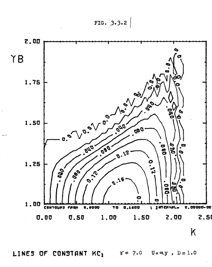
Fig. 3. 3. 2

Growth rate Kci vs K for y ranging

between 5.0 and 9.O. yB = i.0, D = 1.0.

Lines of constant growth rate kc

on a

graph-of YB vs k. y = 7.0, D = 1. 0.

Cases for which the initial condition is a stable eigenvector

which is a solution of the eigenvalue problem. y = 0.0, K

1. O, B= 6.0: Fig. 3. 3. 3

Fig. 3. 3. 4

Fig. 3. 3. 5

Fig. 3. 3. 6

Magnitude of the Fourier transform of the vorticity vs 1 for t = 0.0, 2.5 and 5.0.

Magnitude of the vorticity vs y for t=0.0 and 5.0.

Real part of the streamfunction vs y for t = 0 and 5.0.

Energy of the wave vs y for t = 0.0 and 5.0.

Cases for which the initial condition is an unstable

eigenvector. y

=

5.0, k

=

1.25, B = -15.0:

Fig. 3. 3. 7

Fig. 3. 3. 8

Fig. 3. 3. 9

Fig. 3. 3. 10

Magnitude of the Fourier transform of the

vorticity vs 1 for time values ranging between t = 0 and 8. 0.

Magnitude of the vorticity vs y for time values ranging between t = 0 and 8. 0.

Real part of the streamfunction vs y for time values ranging between t = 0 and 8.0.

Energy of the wave vs y for time values ranging between t = 0 and 8.0.

Infinite domain:

Fig. 4. i. i Orientation of crests of the initial condition on

a graph of y vs x.

Couette flow case without inflection point; y = O, B =

0

and yo

5:

Fig. 4. 1. 3

Fig. 4. i. 4

Fig. 4. i. 5

Magnitude of the vorticity of southward-moving wave where lo/k = -2 for time values ranging

from 0 to 8.

Magnitude of the vorticity of southward-moving wave where lo/k = -2 for t = 0 and 8. Note that the wave does not move, so initial and final values are identical.

Magnitude of the vorticity of northward-moving wave where lo/k = 2 for time values ranging

from 0 to 8.

Magnitude of the vorticity of northward-moving wave where lo/k = 2 fot t = 0 and 8. Note

that the wave does not move, so initial and final values are identical.

Couette flow case with 8-effect without inflection point;

y

= O, yo =

5.

Fig. 4. i. 6 PacKet trajectories for lo/k

=

Fig.

4.

1.

7

Magnitude of the vorticity of southward-moving

wave where

lo/k =

-2 for time values ranging

from 0 to 8.

Fig. 4. i. 8 Magnitude of the vorticity of southward-moving wave where lo/k = -2 for t = 0 and 8.

Fig. 4. i. 9 Magnitude of the vorticity northward-moving wave where lo/k = 2 for time values ranging from 0

to 8.

Fig. 4. i. 10 Magnitude of the vorticity of northward-moving wave where lo/k = 2 for t = 0 and 8.

Fig. 4. 1. i1

Fig. 4. 1. 12

Energy of southward-moving wave where lo/k

=

-2 for time values ranging from 0 to 8.

Energy of northward-moving wave where lo/K

=

2 for time values ranging from 0 to 8.

Finite domain

Couette flow case. The initial condition is a Gaussian. yo

=

=

Fig. 4. 1. 13 Magnitude of the Fourier transform of the

vorticity vs 1 for time values ranging between t=O and 8.

Fig. 4. 1. 14 Magnitude of the vorticity vs y for time values

ranging between t = 0 and 8.

Fig. 4. 1. 15 Real part of the streamfunction vs y for time

values ranging between t=0O and 8.

Fig. 4. 1. 16 Energy of the wave vs y for time values ranging between t = 0 and 8.

Couette flow case. The initial condition is a Gaussian. yo

= 5.0, H = 0.75, 10 = 2.67, K = -1.0, B = 0.0, y=0: Fig. 4. 1. 17 Magnitude of the Fourier transform of the

vorticity vs 1 for time values ranging between t=O and 8.

Fig. 4.1. 18 Magnitude of the vorticity vs y for time values

ranging between t = 0 and 8.

Fig. 4. 1. 19

Fig. 4. 1. 20

Real part of the streamfunction vs y for time values ranging between t=0O and 8.

Energy of the wave vs y for time values ranging between t = 0 and 8.

Couette flow with P-effect. The initial condition is a

southward-moving Gaussian. ye inside the domain and yT

outside the domain. yo = 10.5, H = 2.0, 1o

=

vorticity vs 1 for time values ranging between t=O and 3.

Fig. 4. 1. 22 Magnitude of the vorticity vs y for time values

ranging between t = 0 and 3.

Fig. 4. 1. 23 Real part of the streamfunction vs y for time values ranging between t=O and 3.

Fig. 4. 1. 24 Energy of the wave vs y for time values ranging between t = 0 and 3.

Fig. 4. 1. 25 Magnitude of the Fourier transform of the

vorticity vs 1 for t = 0, i. 5 and 3. 0.

Couette flow with O-effect. The initial condition is a

northward-moving Gaussian. yc and ys inside the domain.

yo = 8.0, H = 2.0, 10 = 2.0, y = 0.0, = 1. O, B 0.0; yc z 6.0, yT O 16.0.

Fig. 4. 1. 26 Magnitude of the Fourier transform of the

vorticity vs 1 for time values ranging between t=O and 8.

Fig. 4. 1. 27 Magnitude of the vorticity vs y for time values

ranging between t = 0 and 8.

Fig. 4. 1. 28 Real part of the streamfunction vs y for time

values ranging between t:O and 8.

Fig. 4. 1. 29 Energy of the wave vs y for time values ranging between t = 0 and 8.

Fig. 4. 1. 30 Magnitude of the Fourier transform of the

vorticity vs 1 for t=O, 2, 4 and 8.

Couette flow with P-effect. The initial condition is a

northward-moving Gaussian. ye outside the domain, YT inside the domain. yo = 8.0, H = 2.0, 10_o = O, y

=

0.0, k = 1.0, B =20.0; Yc

z

Fig. 4. i. 31 Magnitude of the Fourier transform of the

vorticity vs 1 for time values ranging between

t=O and 6.8.

ranging between t = 0 and 6. 8.

Fig. 4. 1. 33 Real part of the streamfunction vs y for time Fig. 4. 1. 34 Energy of the wave vs y for time values ranging

between t = 0 and 6. 8.

Fig. 4. 1. 35 Magnitude of the Fourier transform of the vorticity vs 1 for t=O, 2 and 4.

Fig. 4. 1. 36 Magnitude of the Fourier transform of the vorticity vs 1 for t=6 and 8.

Couette flow with O-effect.The initial condition is a

southward-moving Gaussian. ye and yT outside the

domain. yo = 8.0, H

=

-1.0, B = 75.0; yc z -7.0, yT Z 68.0.

Fig. 4. 1. 37 Magnitude of the Fourier transform of the

vorticity vs 1 for time values ranging between t=O and 6.4.

Fig. 4. 1. 38 Magnitude of the vorticity vs y for time values ranging between t = 0 and 6. 4.

Fig. 4. 1. 39

Fig. 4. 1. 40

Fig. 4. 1. 41

Fig. 4. 1. 42

Real part of the streamfunction vs y for time values ranging between t=0 and 6. 4.

Energy of the wave vs y for time values ranging between t = 0 and 6. 4.

Magnitude of the Fourier transform of the vorticity vs 1 for t = 0 and 2.

Magnitude of the Fourier transform of the

vorticity vs 1 for t = 4 and 6.

Couette flow with s-effect. The initial condition is a northward-moving Gaussian. ye and YT outside the

domain. yo = 8.0, H

=

0.0, B = 75.0; yc z -7. 0, YT 68.0.

Fig. 4. 1. 43 Magnitude of the Fourier transform of the

Fig. 4. 1. 44 Magnitude of the vorticity vs y for time values ranging between t = 0 and 6. 8.

Fig. 4. 1. 45 Real part of the streamfunction vs y for time values ranging between t=O and 6. 8.

Fig. 4. 1. 46 Energy of the wave vs y for time values ranging between t = 0 and 6. 8.

Fig. 4. 1. 47 Magnitude of the Fourier transform of the vorticity vs 1 for t=O and 2.

Fig. 4. 1. 48 Magnitude of the Fourier transform of the vorticity vs 1 for t=4 and 6.

Cases with inflection point:

Fig. 4. 2.i A Q(y) vs y for A2 >O and yc<yB<YTu-Fig. 4. 2. iB Q(y) vs y for A2 >O and YTu<YB<Yc . Fig. 4. 2. IC Q(y) vs y for A2<O and YTu<Yc<YB. Fig. 4. 2. iD Q(y) vs y for A2<O and yB<Yc<YTu.

Stable initial condition in a finite domain: For YTu<YB <yc<Yo. Yo = 3.85, H = 0.75,

10 = 5.0, y = 17.8, k = -2.5, B = -62.3; ye 6 3.65, YTu O 3.41, yB = 3.5, Cgy

-0.16.

Fig. 4. 2. 2 Magnitude of the Fourier transform of the

vorticity vs 1 for time values ranging between t=O and 5.6.

Fig. 4. 2. 3 Magnitude of the vorticity vs y for time values ranging between t = 0 and 5. 6.

Fig. 4. 2. 4 Real part of the streamfunction vs y for time values ranging between t=O and 5. 6.

Fig. 4. 2. 5 Energy of the wave vs y for time values ranging between t = 0 and 5. 6.

Fig. 4. 2. 6 Magnitude of the Fourier transform of the

vorticity vs 1 for t=0O, 2, 4 and 6.

For YTu<yB<Yc<Yo. _{Yo =}

11.0, H = 2.0,1o

= 2. 0, y = 1. 5, k -1.0, B

=

a 8.6, yB 10. O, Cy -0. 24

Fig. 4. 2. 7 Magnitude of the Fourier transform of the

vorticity vs 1 for time values ranging between

t=0 and 6.0.

Fig. 4. 2. 8 Magnitude of the vorticity vs y for time values ranging between t = O and 6. 0.

Fig. 4. 2. 9 Real part of the streamfunction vs y for time

values ranging between t=O and 6. 0.

Fig. 4. 2. 10 Energy of the wave vs y for time values ranging between t = O and 6. 0.

Fig. 4. 2. 11 Magnitude of the Fourier transform of the

vorticity vs 1 for t=O, 1. 5, 3. 0, 4. 5 and 6. 0.

Unstable initial condition in a finite domain:

For yo<Yc<YB<YT. _{Yo = 2.5, H 1.0, 1} o

2. 0, y = 2.5, k = -1.25, B

=

=

0,

Fig. 4. 2. 12 Magnitude of the Fourier transform of the

vorticity vs 1 for time values ranging between t=O and 15.0.

Fig. 4. 2. 13 Magnitude of the vorticity vs y for time values

ranging between t = 0 and 15.0.

Fig. 4. 2. 14 Real part of the streamfunction vs y for time values ranging between t=0O and 15. 0.

Fig. 4.2. 15 Energy of the wave vs y for time values ranging between t = 0 and 15.0.

Fig. 4.2. 16 Magnitude of the Fourier transform of the vorticity vs 1 for t=O, 3 and 6.

Fig. 4.2. 17 Magnitude of the Fourier transform of the vorticity vs 1 for t=6, 9, 12 and 15.

For yo <c<Y <YTu• YO

=

₌

=

=

Fig. 4.2. 18 Magnitude of the Fourier transform of the

vorticity vs 1 for time values ranging between t=O and 16.0 .

Fig. 4. 2. 19 Magnitude of the vorticity vs y for time values

ranging between t = 0 and 16.0 .

Fig. 4.2.20 Real part of the streamfunction vs y for time

values ranging between t=O and 16.0.

Fig. 4.2.21 Energy of the wave vs y for time values ranging

between t : O and 16.0O.

Fig. 4.2.22 Magnitude of the Fourier transform of the

vorticity vs 1 for t=O, 8 and 16. Fig. 4. 2. 23 Real part

t=0.

Fig. 4. 2. 24 Real part t=i. 5. Fig. 4. 2. 25 Real part

t=3. 0. Fig. 4. 2. 26 Real part

t:4. 5. Fig. 4. 2. 27 4.2. 28 Fig. 4. 2. 29 Real part t:6. 0. Real part t=7. 5. Real part t:9. 0. Fig. 4.2. 30 Real part

t=iO. 5. Fig. 4.2.31 Real part

t=12. 0

Fig. 4. 2. 32 Real part t= 15. 0.

of the vorticity vs y and vs x for

of the vorticity vs y and vs x for

of the vorticity vs y and vs x for

of the vorticity vs y and vs x for

of the vorticity vs y and vs x for

of the vorticity vs y and vs x for

of the vorticity vs y and vs x for

of the vorticity vs y and vs x for

of the vorticity vs y and vs x for

of the vorticity vs y and vs x for

13

For yc<YB<YTu<yo' Yo = 5.0, H = 0.75,

10

=

YTu 3.8, YB = 3.5, Cgy Z -0.20.

Fig. 4. 2. 33 Magnitude of the Fourier transform of the

vorticity vs 1 for time values ranging between t=O and 16.

Fig. 4. 2. 34 Magnitude of the vorticity vs y for time values ranging between t = 0 and 16.

Fig. 4. 2. 35 Real part of the streamfunction vs y for time values ranging between t=0O and 16.

Fig. 4.2.36 Energy of the wave vs y for time values ranging between t = O and 16.

Fig. 4.2. 37 Magnitude of the Fourier transform of the vorticity vs 1 for t=O and 0.8.

Fig. 4.2.38 Magnitude of the Fourier transform of the vorticity vs 1 for t=2.4 and 4.0.

Fig. 4.2. 39 Magnitude of the Fourier transform of the vorticity vs 1 for t=6.4 and 8.0.

Fig. 4.2.40 Magnitude of the Fourier transform of the vorticity vs 1 for t=12 and 16.

Fig. 4.2.41 Real part t=0.

Fig. 4.2.42 Real part t=1. 6. Fig. 4.2.43 Real part

t=3. 2. Fig. 4.2.44 Real part

t=4. 8.

Fig. 4.2.45 Real part

t=6. 4. Fig. 4. 2. 46 Real part

t=8. 0.

of the vorticity vs y and vs x for

of the vorticity vs y and vs x for

of the vorticity vs y and vs x for

of the vorticity vs y and vs x for

of the vorticity vs y and vs x for

Fig. 4. 2. 47 Real part t=9. 6. Fig. 4. 2. 48 Real part

t=ii. 2. Fig. 4. 2. 49 Real part

t: 12. 8. Fig. 4. 2. 50 Real part

t= 14. 4. Fig. 4.2.51 Real part

t= 16. 0.

of the vorticity vs y and vs x for

of the vorticity vs y and vs x for

of the vorticity vs y and vs x for

of the vorticity vs y and vs x for

of the vorticity vs y and vs x for

For YTu<YB<Yc<Yo. Yo = 11.,

H = 2.0, k = 1.0

10

=

8. 6, YB

=

Fig. 4. 2. 52 Magnitude of the Fourier transform of the

vorticity vs 1 for time values ranging between t:O and 8.0.

Fig. 4. 2. 53 Magnitude of the vorticity vs y for time values ranging between t = 0 and 8. 0.

Fig. 4. 2. 54 Real part of the streamfunction vs y for time values ranging between t=O and 8. 0.

Fig. 4. 2. 55 Energy of the wave vs y for time values ranging between t = 0 and 8.0.

Fig. 4. 2. 56 Magnitude of the Fourier transform of the vorticity vs 1 for t=O, 2 and 4.

Fig. 4. 2. 57 Magnitude of the Fourier transform of the vorticity vs 1 for t=6 and 8.

For YTu<YB<YC<Yo. Yo = 5.0, H = 0.75,

10

:

=

_o.6.

66.

Fig. 4. 2. 58 Magnitude of the Fourier transform of the

t=O and 14.0.

Fig. 4.

2.

59

Fig. 4.

2.

60

Fig. 4.

2.

61

Fig. 4.

2.

62

Magnitude of the vorticity vs y for time values ranging between t = 0 and 14.0.

Real part of the streamfunction vs y for time values ranging between t=O and 14.0.

Energy of the wave vs y for time values ranging between t = 0 and 14.0.

Magnitude of the Fourier transform of the vorticity vs 1 for t=O, 4, 8 and 12.

LIST OF TABLES

Total energy for the case corresponding to the appropriate figure:

TABLE FIGURE and PAGE TIME INTERVAL

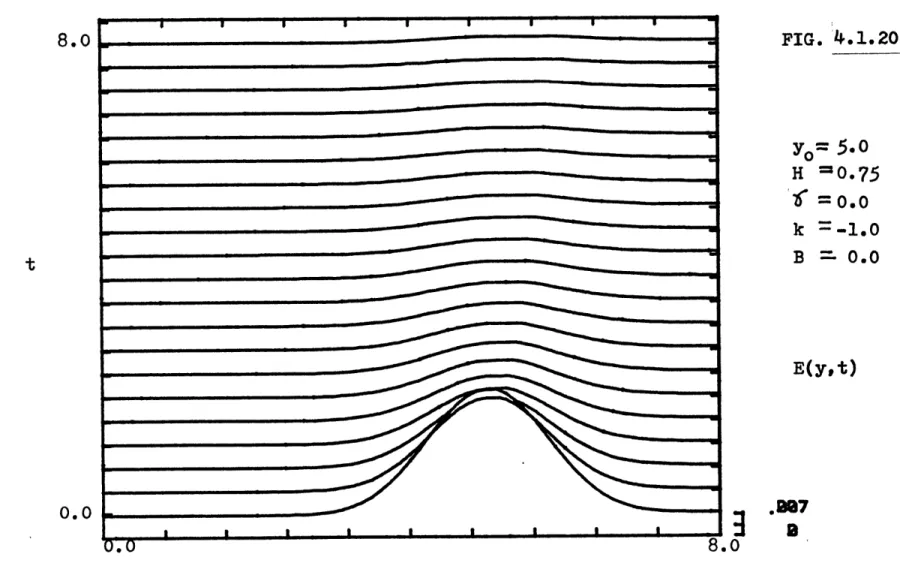
1 3. 3. 6 (0, 8) 2 3. 3. 10 (0,8) 3 4. 1. 16 (O, 8) 4 4. 1. 20 (0,8) 5 4. 1. 24 (0, 3) 6 4. 1. 29 (0,8) 7 4. 1. 34 (0,6.8) 8 4. 1.40 (0,6.4) 9 4. 1. 46 (0,6.8) 10 4.2.5 (0,5.6) 11 4. 2. 10 (0,6) 12 4. 2. 15 (0, 15) 13 4. 2. 21 (0, 15) 14a 4. 2. 36 (0, 16) 14b 4.2.36

(16,32)

17

I. INTRODUCTION

To study the stability of a shear flow to infinitesimal perturbations, what is usually done is to assume that the solution is of the form of a normal mode. To find the general solution of the problem, one has to solve the initial value problem. To achieve this analytically is very complicated and has not been done yet.

Another way to solve this problem is numerically. The results of numerical solutions are usually hard to interpret and analytic results for a corresponding simplified problem are welcome (i.e. asymptotic analysis, wave packet theory...).

In this thesis, the time-dependent evolution of Rossby waves in a sheared zonal flow in a finite domain is studied. The equation used in this model is the linearized barotropic vorticity equation. The solution is considered to be periodic in x. The problem is solved numerically by taking a Fourier transform in y and integrating in time.

In this thesis, it is shown that the equations representing the evolution of an arbitrary initial condition involves the coupling of different wavelengths. This coupling is due to the presence of the walls. The importance of this coupling will be studied by paying a special attention to the evolution of the solution in Fourier space. This is also why the problem is

solved by using a Fourier transform.

Tung (1983) has studied the evolution of an initial value problem where the initial condition is a wave packet with cen-tral wavenumber Ko= (Ko, lo) in an infinite domain

with uniform shear. He has shown that even though the initial disturbances that constitute the wave packet in general do not have a well-defined phase speed, during the later stages of its evolution, the wave packet behaves as a whole, from Kinematic

considerations, as if there exists a well defined phase speed c. He has shown that a packet with positive (10/ko )

has a different trajectory than a packet with negative (10/Ko).For (lo/Ko ) >O, the initial shape moves

first northward untill it reaches a turning point where the group velocity in the meridional direction vanishes. The packet then moves southward, and eventually stagnates at the stagna-tion level which is equal to the critical level. For the case where (lo/Ko ) <0, the packet trajectory is monotone;

the initial shape moves south without changing direction

towards the same stagnation level. Worsham (1983) solving the above problem numerically has shown that his results agree with Tung's analytical results.

For the problem in an infinite domain, no normal mode solu-tions are possible. In a finite domain, normal modes can

deve-lop. We want to study what physical quantities control the onset of this development.

In chapter II of this thesis, the problem formulation is described. In chapter III, the numerical methods are presented

together with a test case. In chapter IV, we first present the results of Worsham (1983) in an infinite domain for a Couette

flow (i.e. uniform shear without 8-effect), then with the P-effect. These results are compared with the finite domain case where first the waves do not interact with the walls and second, where the waves do interact with the walls. In particu-lar, the change in shape of the Fourier spectrum of the vortici-ty is discussed. Further, the effect of the presence of an

inflection point (which is a necessary condition for instabili-ty) is studied. The expressions for the prediction of the sta-gnation level and the turning point found by Tung (1983) are modified in consequence. Also, the theory of overreflection developed by Lindzen and Tung (1978) is applied. The prediction of the position of the critical level combined with the overre-flection theory permits one to explain the time evolution of the wave pacKet.

II. PROBLEM FORMULATION

2.1 Constant shear case

To study the time-dependent evolution of Rossby waves in a zonal flow with shear U(y), the following linearized barotropic vorticity equation is taken as the model equation:

(. + U(y)0_JC (-Uyy)a

=

at

ax

(2. 1. 1)

where W is the perturbation streamfunction and

" (a2/dx2 + a2/aya)2qV2

is the perturbation vorticity.

Equation (2. i. 1) is to be solved subject to the initial condition

S(x,y, t=O)

=

(2. 1. 2) The boundary conditions are

C = 0 (y = O,2D)

(2.

1. 3)

where ( is periodic in x with a period of 2Ta cos 0o;

the length of the zonal circle at latitude O

=

The shear is taken as U(y) : ay. Since Uyy would be

zero, the additional assumption that 9-Uyy is of the

form a(y - b) is made. b is the so-called inflection point,

i.e. the location where the mean vorticity gradient changes

sign.

The resulting equation is then

(L_ ay Lav2V + o(y - b) AI=O

at

ax

ax

(2. i. 4)

To solve equation (2. i. i), we take a Fourier sine transform of

the equation so that the boundary conditions C = O at y=O, 2D will be satisfied. The coefficients of the above partial differential equation are not constant, and once the Fourier transform of the equation is taken, we obtain a system of first order linear differential equations. This is demonstrated here. Let IV = qei kx, then equation (2. 1.4) becomes:

(_ + ayik) (.

k-

_)*

_{+ a(y - b) ik:0O}

at ay

(2. 1. 5)

To be able to satisfy the boundary conditions, let OD

r =

sin

In

= nl/2D ,n=i,2...

n=O

(2. 1. 6) Replace * defined in (2. i. 6) in eq. (2. 1. 5) and also drop the index n:

0 = E ((12+k

+

)A +-

J

+iyk(a(l +k )-a)) sin ly.

Then

2D

(i/D) I sin 1 'y (eq. (2. i. 7))dy = (1'2+k ) _(l t)

0

_at

2D

+ abik;(l',t) +(i/D)E[f sin l'y sin ly dy y ik

1 0

. (1,t) (a(12+ 2a) - a)] = O

(2. 1. 8)

Now sin ly sin l'y

i=

2D 2D

Let A J S y sin ly sin l'y dy = 1/2 1 y dy cos (1-1')y

-O O 2D 1/2 1 y dy cos (1+1')y. O Then if 1 t 1': A 1/2 cos (1-11y ; 2D (1-1') 10 + 1/2 y sin (1-1')y 1 (Also -1') cos 2D Also cos (1-1') 2D = (-i)n - n '

- 1/2 cos(l+l'll I2D (1+1') O D - 1/2 y sin (1+1') 2D (1+1') 0 , and sin (1-1')2D

=0.

o

=

_(l',t)

')

-

(-)n+n'

1

If we use L as a length scale and i/a as a time scale, then equation (2. 1. 9) in nondimensional

*(I', t) :(', t) f (B+yd) ik - ikd) %J.71 1=0 , 141' form becomes: Sik2df(-i) (n+n') '17 (n+n') 2

- (-l)

(n-n') _]

].

(l, t)

(n-n')

=

=

To study the problem without an inflection point,y has to be set equal to zero. Other interesting quantities to study are the energy and the vorticity.

i) Energy averaged over one cycle in x:

x E(y, t)

=

ax

ay

Let Vt(x,y,t)

=

=:

A: ikeikx (y, t)

Re

At

(Re af2

=

K2 sin2Kx *R2

+ K2 cos2Kx *2I

+ 2 K2 cos Kx sin Kx *R

*I-Let J(y,t) = E sin ly *(l, t). 1=0 Then V(x,y,t) = ei K x Z ei l y F(, t); 1= -O where = 1 1 O; F(1, t) [ Also AT

=

where G(l,t) = 1 (l,t)/2i, for all 1. So

A= eikxi W where W = Ee i l y G(1,t) Av 1= -a

(Re AT

:

aY

25

(Re AM 2 = sineKx WR2 + cos2 x Wia

+ _{2 sin Kx cos Kx WR WI}

Collecting terms, we get:

E(y,t) = 1 E(x,y, t) dx

(2/Rk) 0

=

The total energy, i.e., the energy integrated over x and y

is defined in the numerical methods section (section 3. 3).

ii) Vorticity: The vorticity

S(x,y,t) = v2 (x, y,t)

= ei k x (-K2 + 2 (yt)

ei K x w(y,t).

In terms of sine Fourier transforms:

w(y,t) Z= sin ly w(l,t) 1=0 we have:

w(l,

=

A_(l',t) w(l',t)

((B

I

at

W

ZE

1=0

"

(n+n')

1l'

(n-n')

(2. i.

12)

Instead of taking a Fourier sine transform to solve the

above problem, it is possible to take a complex Fourier

trans-form provided

"(-l,t)= -

"(1,t).

This condition

is

demonstrated in the appendix.

2.

2 Normal mode problem for the constant shear case

The evolution of an arbitrary initial disturbance into a

normal mode is studied. This solution is of the form

eik(x-ct).*(y)

and

c

=

cr

+

ic

To know what

values to give to the parameters of the problem so that it is

unstable (i.e., c

> 0), a study of the normal mode

eigen-value problem and its stability is done.

The eigenvalue problem is solved numerically. A description

of the numerical scheme is given in section 3.

3.

Only the

equation and its nondimensional counterpart are given here.

Let ~:ei k(x-ct) *(y), then eq. (2. i. 5) becomes:

(ay - c) fd* - 2 +

a(y-b)

(2. 2. i) If, again, as before, L = length scale and i/a = time scale, then eq. (2. 2. 1) becomes:

(y-c) ( 2 - 23 Y(Y-B) * =0 dy

(2. 2. 2)

III. NUMERICAL METHODS

3.1 Initial condition

The initial condition used throughout most of this work is a Gaussian distribution, i.e. in physical space the function is of the form

expf-(y-yo)2/4H2] expfiloyl.

H is given values so that the Gaussian fits inside the domain, i.e. is zero at the boundaries. Varying H can produce a wider or narrower function. The narrower the function is in physical space, the wider it is in Fourier space. To apply wave-packet theory to the problem (Tung, 1983), the function has to be

peaked in Fourier space, but it should not be too peaked becau-se the Gaussian function at t=O in physical space should be

localized. This is because the Gaussian function is considered as an "arbitrary" initial condition, and therefore, at t = 0, it should not resemble an eigenmode which, in general, has a global structure.

In an infinite domain, the Fourier transform of a Gaussian is a Gaussian. In a finite domain, this is not the case, but if the initial condition is as described above, then one can

con-sider the function as "Gaussian-like" with 1o as central

frequency and yo as central position in physical space.

3. 2 Constant shear case

The program mainly consists of six parts.

i. Take the fast Fourier transform (FFT) of the initial condition which is a Gaussian in physical space for the

vorticity. The FFT has N+i points say.

2. Calculate the corresponding streamfunction in Fourier space.

3. Integrate the streamfunction in time.

In order to do that, it is necessary to solve a system of N ordinary linear differential equations for a time

interval At = tn+i - tn. To do this, use is

made of Gear's method. Gear's method is used to insure numerical stability. It is also used to solve stiff

equations (Raphson and Robinowitz, 1978, p. 228). A

subroutine from the NAG library was used for this.

4. Calculate W - G(, t) and w (see eqs. 2.1.11 and

2. 1.12 respectively).

5. Take the inverse of the Fourier transforms 9, W,

w at each tn and calculate E(y,t) at each tn.

6. Calculate E(t) at each tn. E(t) is defined as:

M-i

E(tn)

₌

d 2 i=2

+ Ay E(yM,t') ₎ 2

where M = N/2.

At each timestep, the results are plotted out for the following quantities: If (x=O, i, t) I, Iw(x=O,y, t) I,

Re(T(x=O,y,t) and E(y,t). Also, at each timestep, a plot of Re(r (x,y,t)) in three dimensions is available.

In theory, 1 varies between zero and infinity. To execute a numerical computation, 1 has to be cut off. Consequently, 1 varies between zero and a finite value which will here be

defi-ned as 1MAX . If the amplitude of the function in Fourier

space becomes significantly different from zero around IMA_X

the integration in time has to be stopped to avoid aliasing. An example of this is shown on Figure 4. i. 36.

There is also a limit on the resolution. In most of the

computations, N = 128, which means that in the physical domain

y e O,2D], there are 64 intervals, and the same number is

used for the antisymmetric extension y e E-2D,03.

There-fore, waves smaller than (D/16) cannot be represented.

To verify the accuracy of the numerical integration, dif-ferent values of the local error for Gear's method have been taken. The values for the tolerance was first set to 10-4

and then 10-8 . Cases for which the total energy decayed

continuously in time showed the lowest accuracy. In general, for a qualitative study of the behavior of the problem, a

tolerance of 10- 4 was more than enough. The need to set a

higher tolerance depends also on how long the integration is

executed.

3. 3 Normal mode problem for the constant shear case

a) Eigenvalue problem

Rewriting equation (2. 2. 2) we have:

y[ d2& - k2*3 + R(y)* =

dy

cEd2~ _{- K}2₃

dy

(3. 3. 1) where R(y) = y(y-yB).

If we use a second-order finite differencing to evaluate

d2 n+ - 2n + *n-i

. " 0 n+i dy

(Ay) 2

then the L.H.S. of the above equation becomes:

Yn I *n+i-2n,+*n-i - K2 n] (Ay) 2 + Rn *n or multiplying by (Ay) 2: yn *n+i+*n 1- 2 yn K2 (Ay) 2yn + Rn(Ay) ₂ + Ynn-i " Also, *o = 0 and *N+i = 0 from the boundary

conditions.

Let V_n

=

In matrix form, we then have for the L. H. S.:

Vi Yi Y₂ V2 Y2 *2 Yn Vn Yn *n YN VN

*N

which becomes after multiplication by (Ay) 2 :

C [ n+i + 1-2- 2 (Ay) 2 I n + n-i

Let Z -2 - 2 (Ay)2 , then the R.H.S. is:

Z i 91

i Z i *2

c cP

i Z

Finally, M

=

To solve this problem, a subroutine from the NAG library was used to find the eigenvalues c and also the eigenvectors * if needed. With this program, eigenvalues for the problem without an inflection point and with an inflection point can be

found. Recall that the inflection point is equal to YB'

The eigenvalue problem without an inflection point is

always stable. This follows from the Rayleigh-Kuo theorem. Only neutral modes are obtained numerically with phase speeds

smaller than zero. With the vorticity gradient P- Uyy = a(Y-YB),

the Rayleigh-Kuo theorem says that a necessary condition for instability is that the inflection point lies inside the

domain. Fjortoft's theorem can also be applied. The short-wave cutoff for instability can be shown to be

(y-

/4D2

1i/2= kMAX

(see Pedlosky (1979) for a similar derivation). For the eigen-value problem with an inflection point, a graph of the growth

rate (kci) versus the wavenumber for different values of

y is shown on Fig. 3. 3. 1. This diagram is for a nondimen-sional domain of size = 2. The most unstable wave occurs when

yg is at the center of the domain. Lines of constant growth

rate are shown in Fig. 3. 3. 2. The zero growth rate line is very wiggly; this should not be the case and is due to an insuffi-cient amount of data points for the plotting routine. This

graph is only meant to give a qualitative idea about the insta-bility properties.

b) Eigenvector as an initial condition

To test the numerical method, the initial condition is set equal to an eigenvector which was found by solving the eigen-value problem. The eigenvectors in the case without an

inflec-tion point and with an inflecinflec-tion point were both calculated. An eigenvector given as an initial condition should always

remain a solution to the initial value problem.

Figure 3. 3. 3-4 illustrate the magnitude of the Fourier transform of the vorticity and the magnitude of the vorticity. These should both be conserved in time.

Figure 3.3.5 illustrates the real part of the streamfunc-tion. The oscillation in time is present because the complex

streamfunction is of the form expl-iKcrt3. Figure 3. 3. 6

shows the energy as a function of y and t which should be con-served in time. In an eigenvalue problem the accuracy of the eigenvalue is larger than that of the eigenvector. Since there is some error in the eigenvector, it will need some time to

adjust to the initial value problem. This is the main reason for the discrepancies observed in the figures mentioned above.

Another check is that the total energy E(t) has to be con-served. This is the case (see Table i). The phase speed cr could also be verified using x vs y vs Re(vort(x,y,t,)) dia-grams.

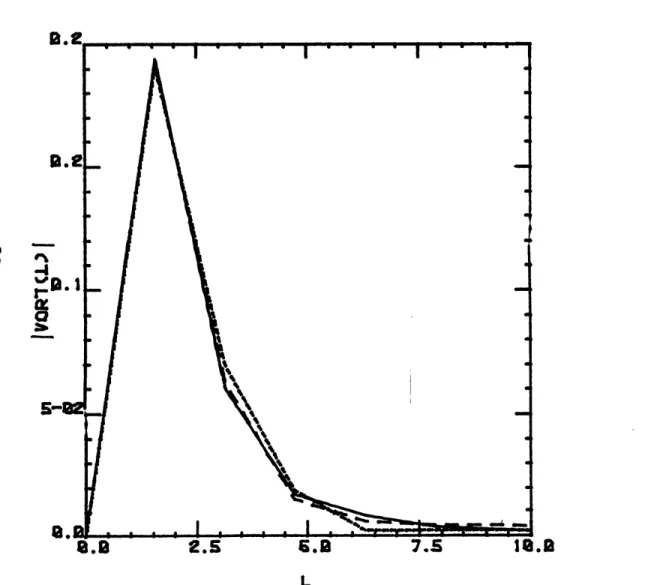
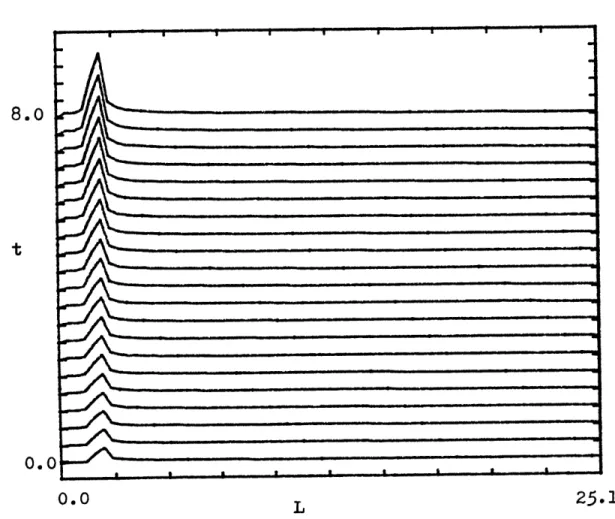
Figures 3. 3.7-ii illustrate the unstable eigenvector. The same variables as for the case above are illustrated. The total

energy grows like exp[2Kci t] which it has to (see Table 2).

Here also the phase speed cr turned out to be the same as predicted.

FIG.

3*3.*

0.25

KC

0.20

O.

I

0.10

0.0

o.0 0-

_0.0

YBtI. 00

0.5

1.0

1.5

2.0

-1-

5.0

6.0

7.0

8.0

9.0

U=O(y

37

2.5

FIG.

.3.3.2

2.00

YB

1.75

1.50

1.0

0

Cua ULrns firn 1.wo o TO 0.luso

0.00

0.50

LINES OF

CONSTANT

1.00

KCz

1.50

Tr= 7.0

2.0o

U=oKy , D= 1.0

3

FIG.

_3.3.3

'g-=

0.0

k =1.0

B

=6.o

le 0. 0, 100.

51

T

=

0.0

T

=

2.5

T

=

_{5. 0}

w8'

o*9=~

g

it

0"0= z

oo=

.*-0

'oa.

O

ee

-Ct

.'a

•

•

-as

Q.9

2.9

•

0

FIG. 3.3.5

Y'=

0.0

k= 1.0

B=6.0

-

T=0.0

~---

T-

5.

₀

0

0

FIG.

3.3.6

T =

k

B=

0.0

1.0

6.0

-T = 0.0

_T

FIG.

3.3.7

8.0

S=

5.0

1.25

B

₌

-15.0

t

.Vort(L)l

0.0

0.0

L

25.13

0'8

0.0

0"0

I(VYL)OAI

oo'

•

.

08

01A

9.cSc

0

0

0

0

11 ii i YiYi i i iihi I i tiii i l ii IL ill i i iii 11

0

-0

FIG.

3-3.9

f=5.o

k

=1.25

B :

-15.0

Re

sf(y, t)

8.0

8.0

4

t

0.0

L

0.0

8

FIG.

3.3.10

8.

5.0

k

1.25

ONIII

B = -15.0

E(yt)

0.0

0.0

8.0

S]

FIG. 3.3.11

15,

k

=1.25

SaB

tt

=2.0

S----

t

=

4, 0

--- t= 6.0

---

t=8.0

IV. RESULTS AND DISCUSSIONS

4. i Constant shear case without an inflection point 4. 1.1. Infinite domain.

For the constant shear case in an infinite domain with 8-effect, the solution in moving coordinates is (Tung

(1983)):

OD

S (i/a2T)! ei k 4+inM

-O ((k, M,T) dM

(4. 1. 1) where 4 = x - ayt, :=Y , -=t and

N aN

S(k,M,T)

=

ak

[tg-i(at-M/k) + tg-i(M/k)]3

(4. 1. 2)

If one takes the magnitude of both sides of the above equation, one obtains: It (k,M,) I I o(k,M)I (4. 1. 3) In fixed coordinates : (x,y,t) - (i/wT)eiKxf ei l y ( (, l+akt, t)dl and equation (4. 1. 3) becomes:

I (k, l+akt, t)I

=

(4. 1. 4) Equation (4. 1. 4) shows that IgI depends on l+akt.

displaced in time by the shear at a uniform rate ak.

Consider the evolution in time of the central wavenumber

lo(t) of the wave-packet (see Figure 4.1.1). If

(1₀(0)/K) >0 then the orientation of the crest of the wave at t=O is north-west. The effect of the shear will then be to

increase the y-scale of the wave (i.e. decrease lo), when

the orientation is north-south, the y-scale is infinity and 1

=0.This

lo( 0 ) - aKt*=O.

Thus t*=l1(0)/aK.

When the orientation becomes north-east, then the scale of y decreases i.e. 1101 will increase.

If (lo(0)/K)<O,the orientation of the crest of the wave is north-east. The effect of the shear is to decrease the y -scale and hence increase the wavenumber.

a)Couette flow

For the Couette flow 8 =0, the effect of the shear

is the same as described above since equation (4. i. 4) does not depend on 8. It is also possible from the differential

equation to show that I (x,y,t) I is conserved with

time. This is illustrated in figures 4. i. 2 and 4. 1. 3 for which (l 0/k)>O. Figures 4. i. 4 and 4. 1. 5 also show that

I (x, y, t) I is constant for the case (1o/K) <0. These

figures were calculated by Worsham (1983).

The kinetic energy density averaged over x for one wavenumber 1 is:

(1/4) (k2 + 12)

I

* - (k,1+at,t) / (k +12).

Therefore, using eq. (4.1.4):

E = (1/4) 1Co(k, l+akt)1 2/(k 2 + 1).

As before, consider the time-evolution of the central wavenumber

lo(t) of a wave-packet with small spectral spread. Then substitute 1 - l(t) = lo(0) - akt in E.One obtains

E " EK2 + (1o (0)-akt) 2 3-1 .

When (1o(0)/k)<0 the energy always decays and when

(10 (O)/K) >O the energy increases untill t = t* and then

decreases. t* is the same as defined above.

b) Couette flow with a-effect

When 8 is different from zero, the waves can move in the y direction. Tung (1983) studied the evolution of a

wave-packet in an infinite domain where the initial spectrum

Co(k, 1) is peaked about the central wavenumber ko (ko,1o). There is a small spectral spread AKo

about the central wavenumber. He showed that

Yc = Yo - 8/(K2 +1)

and

YT = Yo + 8(lo 2/ 2/ ) (k2 + 2

)

We recall that yo is the position of the centroid of the Gaussian initial wave-packet. yc is the critical level

and is the point where the wave-packet eventually stagnates. It

is determined by the location where U(y)-c = O. c is the

baro-tropic wave speed in the absence of shear. It is called the nominal phase speed of the packet. Even though the initial

disturbance (here a Gaussian distribution) that constitutes the wave-packet, in general do not have a well-defined phase speed, Tung (1983) has shown that during the later stages of its

evolution, the wavepacket behaves as if there exists a well -defined phase speed c. Worsham (1983) has shown numerically that this is the case.

YT is the turning point and is the location where the group velocity in the meridional direction changes sign. This

occurs at at = lo/K. The group velocity is

Cgy = 2Kol / (K2+12) 2

Figures 4. 1. 6 to 4. i. 12 were computed by Worsham (1983).

Figure 4. i. 6 illustrates the packet trajectories for lo/K

=

f 2. For lo/K=2, the wave-packet is moving northwards

untill it hits the turning point and then moves south towards

the critical level. For lo/K = -2, the wave-packet moves

south towards the critical level. Figures 4. 1.7 - 4. 1.8 illus-trate the magnitude of the vorticity of a wave packet moving south towards the critical level. Figures 4. i. 9 - 4. i. 10 illustrate the magnitude of the vorticity of a wave-packet moving north, hitting the turning point and then moving south

towards the critical level. Figure 4.1.11 illustrates the

energy for a southward-moving wave-packet. The energy always

decays as discussed before. Figure 4. i. 12 illustrates the

energy for a wave-packet moving north. When the wave moves north, the energy increases and when the wave moves south, the energy decays. The reasons for the behaviour of the energy is basically the same as the one described for the Couette flow.

4. 1.

2

a)Couette flow (=o0)

For the Couette flow in a finite domain, it is also

possible to show that JI (x,y,t) I is conserved. This can

be seeson figures 4. i. 14 and 4. 1. 18 which illustrate

I (x=O, y, t) I for (lo/K) >0 and (lo/k) <0 respec-tively.

Figures 4. 1. 16 and 4. 1.20 show the evolution of the energy E(y,t) for (lo/k)>O and (lo/k)<0 respectively. (Also

see tables 3 and 4) The behaviour of the energy is the same as the one predicted for the Couette flow in an infinite domain. The waves in physical space do not move so that the walls at

y=O and 2D are basically not felt.

The magnitude of the Fourier spectrum of the vorticity is illustrated in figures 4. i. 13 and 4. i. 17 for (lo/) >O and

(lo/k)<O. Consider first the case (lo/) <0. Roughly one

can say that the behaviour of the function in Fourier space is the same as for the infinite domain. The change in 1 with time is due to the shear and was described in section 4. i. ia. One has also to consider the fact that the Fourier spectrum is made

up of values of 1 e EO,03 and also 1 e E-o,03. The

function for 1<0 is the antisymmetric extension of the function for 1>0. It is the inverse of the Fourier transform of these two functions which make up a function in physical space which satisfies the boundary conditions. In a finite domain, there is an interaction between different wavenumbers. This is due to the coupling terms in the system of differential equations. This coupling which is present because of the walls can explain the development of longer waves of the spectrum which is

obser-ved as time increases (i. e. broadening of the Fourier spectrum

towards smaller wavenumbers). The longer waves are the first ones to feel the walls.

Consider the case for which (lo/k)>O. At t=0, the

ini-tial condition has a Gaussian-like shape. As t increases, since

both the function and its virtual image move towards 1=0, the functions while passing each other will superpose. So the function which was initially in the region 1<0 will now be in the region with 1>0 and vice versa. Therefore, the effect of the shear on the scale of 1 in a finite domain is roughly the same as for the infinite domain (i.e. if one excludes the broadening effects).

Only transient waves make up the Fourier spectrum, i.e. the 1-scale is continuously changing.

Also, one can conclude that the decay of the wave is asso-ciated with the function in Fourier spectrum which is moving towards larger l's. This particular structure will be called the part of the Fourier spectrum associated with the decay of the wave.

b) Couette flow with B-effect

Consider first the cases where the effects of the walls are almost not felt. This is possible because of the presence of Yc and yT.

In a finite domain, one can place the walls so that yc and yT are inside or outside the domain.

When only yc is inside the domain and yc is to the south of yo (where yo is the centroid of the wave

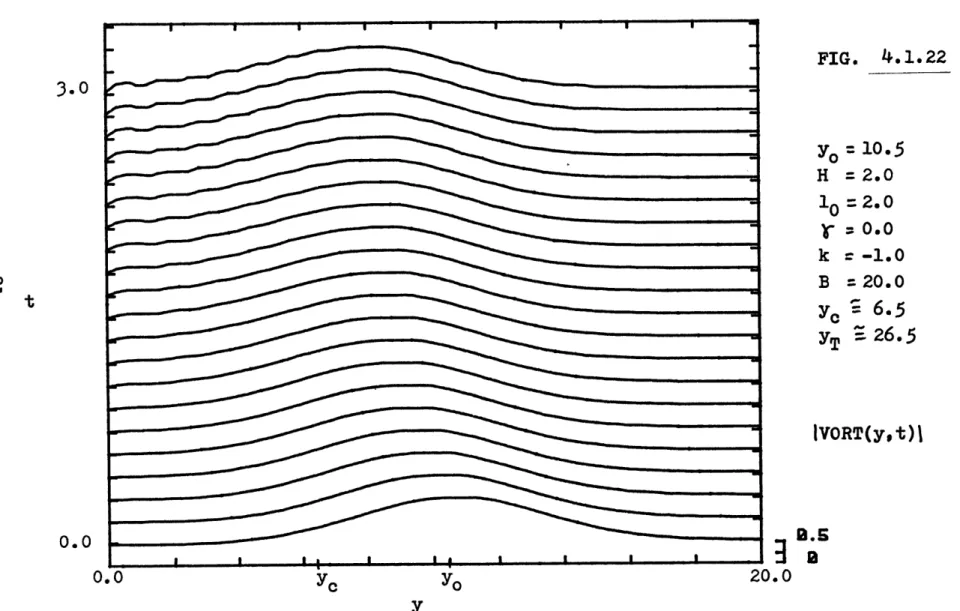
-packet) and the initial group velocity of the wave-packet is negative, then the centroid of the wave-packet will stagnate at yc and will not be able to travel to the wall. This is shown in figure 4. i. 22. As time increases, small scale struc-tures appear. These are due to the presence of the wall. The tail end of the packet feels the wall and moves very slowly as time increases (i.e. it is only when t -> m that Cgy ->0). The behaviour of the wave is basically the same as for the infinite domain case. As expected, the Fourier spectrum is the same as for the Couette flow (0=0).

The energy of the wave-packet decays as it moves south (see figure 4. 1.24 and table 5). This is due to the effect of the shear acting on the wave-packet near the stagnation level.

If yc and yT are both inside the domain, i.e.

Yc <Yo YT

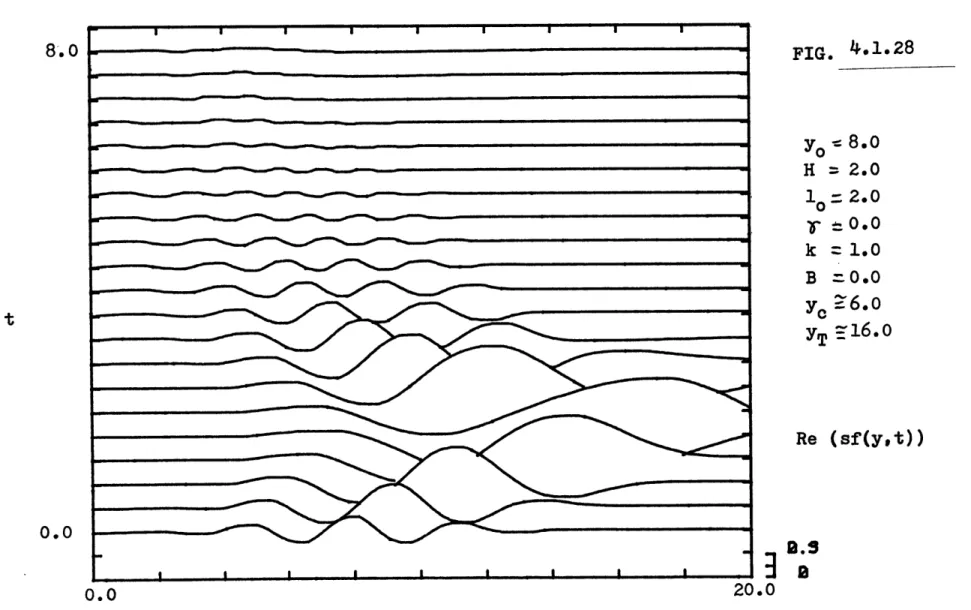
and Cgy(t=O)>O, then the wave-packet moves north untill it hits the turning point and then moves south and stagnates at

the critical level. Again in this way the wave-pacKet did not enter in contact with the walls and one obtains the same over-all behaviour as for the infinite domain case. Figure 4.

.

Consider now cases where the presence of the walls is felt considerably.

If YT

is inside the domain

(O<yo<yT<2D)

and

Cgy(t=O)>O, then the wave-packet moves north untill it hits the turning point and then moves south and feels the left wall. Figures 4. i. 31-4. 1. 36 illustrate this case. The energy

increa-ses as the wave goes north and then decreaincrea-ses as the wave goes

south (see also table 7). It then increases again as the wave

goes north and increases and decays in a "harmonic fashion". By bouncing back and forth against the walls, eigenvectors are set up. Since the eigenvectors are neutral for this

problem, waves with different phase speeds are present and all have a phase speed cr<Umin. Before and untill the

the same shape as for the case without walls considered before. When the waves enter in contact with the walls, distinct

smal-ler wavenumbers develop. As the neutral waves are being set up, the part of the Fourier spectrum associated with the decay

of the wave fades away (it is smeared out over larger and larger wavenumbers).

The development of the smaller wavenumbers as mentioned before is due to the fact that the normal modes have a definite

structure in the y domain. There is not just one peak but

several because of the presence of several neutral waves which each have a different phase speed. The left side of the domain in physical space is a lot more wavy than the right side. This seems to indicate that some wavelengths feel a turning point which is to the left of YT(lo).

If both yc and yT are outside the domain, i.e. yc < 0 < yo < 2D < YT

then the wave-packet will come directly in contact with the wall. Consider first the case (10o/)<O. As time evolves,

two distinct structures appear one after the other in Fourier space. At first, only the part of the Fourier spectrum asso-ciated with the decay of the wave is present; as for the

Couette flow, this is due to the effect of the shear. When the wave-pacKet in physical space enters in contact with the wall, distinct wavenumber peaks appear for the lower wavenumber part of the spectrum. This structure of the spectrum persists while

the part of the spectrum associated with the decay of the wave fades away as for the case described just before.

Figures 4. 1. 37-4. i. 42 illustrate this case. The total energy decays while the wave is going south, then increases once the wave has entered in contact with the wall. After that, the energy decays and again increases and decays in a "rythmic fashion" (see table 8). The fact that the energy increases and decays in a so- called "rythmic fashion" suggests the presence of several neutral waves. The initial condition has a spread of

wavenumbers around 1o . The walls can contain structures

with different wavenumbers each thus having a different phase speed. What we observe in physical space as well as in Fourier space is a superposition of these waves. Again, as in the

previous case cr(l) should be smaller than Umin for a

solution to exist. In the case where several normal modes are present, it is not possible to determine numerically what

cr is.

Consider now the case (lo/k) >0. Figures 4. 1. 43-4. 1. 48 illustrate this case. For the first seven timesteps, one can again observe the same general behaviour of the Fourier

spectrum as for the Couette flow with (lo/K)>O. For the

latest timesteps during this time, one can see the development of distinct wavenumber peaks and as time goes on this structure

becomes more and more developed (i. e. normal modes are

associated with the decay of the wave fades away. As the wave goes north untill it hits the wall, the energy increases (this is consistent with the Couette flow case). Then the energy decreases untill the wave hits the left wall and increases again, then decreases and finally increases and decays in a "rythmic fashion". This also indicates the development of normal modes. See also table 9. Again, Cr<Umin.

Comparing the solution for (lo/K)>O and (lo/K)<O, one

can conclude that they have the same general form. The final Fourier spectra are similar as well as the solution in Fourier

space. This is to be expected since ye and yT are

outside the domain (so that the waves have no obstacles) and the initial conditions are the same.

In the three last cases mentioned above, the presence of the walls cause the development of distinct wavenumbers in the lower wavenumber part of the spectrum which does not shift in time, indicating the presence of a definite structure in

physical space which is a superposition of normal modes with different phase speeds.

NORTH

(10

(0O)/ko

>

WEST

o,- (1

/k)

(0

EAST

SOUTH

FIG. 4.1.1

0

0

0

0

0

0

0*

0.0

8.0

O

-0

0.0

t

8.0

Figure 4. 1.4

_

1.5

1/k = 2.0

Yo

= 5.0

'C

= 0.0

1.0

B

:0.0

t

=0.0

t

=8.0

0.0

-20.0

-13.3

-

6.7

0.0

6.7

13.3

20.0

Y

0.0

t

Figure

4.1.8

1.5

1.0

0.0

- 0.5

1

SIVORTICITY(

Y, t)l

y

50

OTV1-E

OZEtoId

0*8 =I-

%

= I

o*o

0

0

0

0

0

0

0

S

a

0

0

0

0

0

0

0

0

0

0.0

0

0

Figure

4.1.12

0.0

t

0

~

0-

0

0I

8

0

tt

0.0

FIG.

411.1.13

Yo

H=

5.0

0.75

1

=

2.67

=

0.0

k =

1.0

B

0.0

I

(VORT (L, t)

4

0

0

0

0

0

0

0~

0

000

FIG. 4.1.14

yO

5.0

8.0

H

0.75

10

=2.67

Ik 1.0

B

0.0

t

VORT(y.t)

0.0

0.0

8.0

0

0

0

0

0