Assessment of light water reactor power plant cost and ultra-acceleration depreciation financing

ULTRA-ACCELERATION DEPRECIATION FINANCING by

Sadek Abdulhafid El-Magboub and David D. Lanning MIT Energy Laboratory Report No. MIT-EL 78-041

September 1978

Report from the joint Nuclear Engineering Department/Energy Laboratory Light Water Reactor Project sponsored by the U.S. Energy Research and Development Administration (now Depart-ment of Energy).

POWER PLANT FIXED COST AND

ULTRA-ACCELERATED DEPRECIATION FINANCING by

SADEK ABDULHAFID EL-MAGBOUB DAVID D. LANNING

September 1978

Energy Laboratory in association with the Department of Nuclear Engineering Massachusetts Institute of Technology

ABSTRACT

Although in many regions of the U.S. the least expensive electricity is generated from light-water reactor (LWR) plants, the fixed (capital plus operation and maintenance) cost has increased to the level where the cost plus the associated uncertainties exceed the limits deemed

acceptable by most utilities.

The operation and maintenance cost has increased about 25% annually during the early 1970s. The main causes are increased requirements due to safety, environmental, and security considerations. The largest

improvement is co-location of units, which gives up to 37% savings in O&M cost.

The rising trend of LWR capital cost is investigated. Increased plant requirements of equipment, labor, material, and time due to safety, environmental, availability, and financial considerations and due to lower productivity and public intervention are the major causes of this rising cost trend. An attempt is made to explore the elements of a comprehensive strategy for capital cost improvement. The scope of the strategy is divided into three areas. The first includes improving the current design, project management, and licensing practices. The second area, standardization, is found to reduce cost by 6 to 22% through

Duplication and Reference System options. Due to lack of commercial experience, the status of Flotation is not clear. Replication presents no significant improvement. The third area is improved utility structure and finance. Electric utilities with improved organizational structure can save up to 30% of their regional average capital cost. A proposed option of Ultra-accelerated Depreciation (UAD) financing is

investigated. In addition to increasing the availability of capital, this UAD financing, unlike other financial schemes, is expected to

decelerate future rise of electricity prices. A computer code, ULTRA, is developed to assess this option.

Most of the information presented in this report has come via the Utility and Industry Survey described in Chapter II. We appreciate those who supplied us with positive responses, those who made comments on our

Interim Report, and those who advised us about the various aspects of this study. Financial support for this project was received from the U.S. Department of Energy.

We wish to acknowledge the cooperation of our colleagues at MIT, especially those who worked on the LWR Program, and in particular

Professor David J. Rose of the Nuclear Engineering Department, and David O. Wood of the MIT Energy Laboratory for their useful input.

We also appreciate the assistance of Rachel Morton, the MIT Nuclear Engineering Department computer code librarian, for her help with CONCEPT code, and Debbie J. Welsh of the MIT Nuclear Engineering Department for her secretarial work.

TABLE OF CONTENTS Page Abstract ₂ Acknowledgments 3 Table of Contents 4 List of Tables 9 List of Figures 11 I. Introduction 13

II. Assessment of U.S. Survey Data 21

2.1 Data from the Survey of U.S. Nuclear Industry 23

III. Capital Cost Estimate 29

3.1 Basic Definitions 29

3.2 Use of CONCEPT Code, Phase 5 32

3.2.1 Accuracy of CONCEPT Code, Phase 5 35

3.3 The Capital Cost Base Case 36

3.3.1 Capital Cost of LWRs 36

3.3.2 Capital Cost of Coal-Fired Plants 41

3.3.3 Assessment of Base Case Data 41

IV. Present Trend of Capital Cost 43

V. Contributions of the Capital Cost Elements ₅₃

5.1 Equipment Contributions 55

5.1.1 Capital Cost Sensitivity to Equipment Cost 58

5.2 Labor Contributions 59

5.2.1 Capital Cost Sensitivity to Labor Cost 61 5.3 Contribution of Plant Construction Materials 66

TABLE OF CONTENTS (continued)

Page

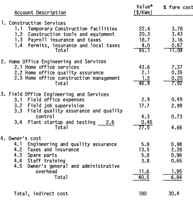
5.4 Contribution of Indirect Costs 68

5.5 Time Contribution 72

5.6 Summary 87

VI. Causes of Increased Capital Cost 90

6.1 Increased Unit-Cost 90

6.1.1 Escalation of Physical Capital Cost Elements 97

6.1.2 Escalation of Time Cost 97

6.1.3 Escalation and Plant Capital Cost 98

6.2 Increased Requirements 100 6.2.1 Size-related Requirements 103 6.2.2 Availability Considerations 104 6.2.3 Safety Considerations 106 6.2.4 Environmental Considerations 108 6.2.5 Lower Productivity 110 6.2.6 Public Intervention 114 6.2.7 Financial Requirements 114

6.2.8 Summary of Increased Requirements 118 VII. Possible Alternatives for Capital Cost Improvement 119

7.1 Optimization of Current Practices 120

7.1.1 Design Optimization 120

7.1.2 Improved Project Management 123

TABLE OF CONTENTS (continued) Page 7.2 Standardization 126 7.2.1 Flotation 129 7.2.2 Duplication 138 7.2.3 Replication 149 7.2.4 Reference Systems 151 7.2.4.1 NSSS Reference Design 152

7.2.4.2 BOP Reference Design 155

7.2.4.3 The Island Concept 158

7.2.4.4 Standardized Modular Design 163

7.2.5 Summary 165

7.3 Licensing Procedures 168

7.3.1 Early Site-review 169

7.3.2 Limited Work Authorization 171

7.3.3 Periodic Freeze on Regulatory Changes 175 7.4 Improved Utility Structure and Finance 178

7.4.1 Organizational Improvement 179

7.4.1.1 Size Characteristics 184

7.4.1.2 Functional Characterizatics 186

7.4.2 Alternative Financial Methods 191

7.4.2.1 The Conventional Method 192

7.4.2.2 The CWIP Method 195

7.4.2.3 The UAD Method 199

7.4.2.4 Summary of Financial Methods 216

7.5 Conclusions 218

VIII. Factors Limiting Capital Cost Improvement 220

8.1 Size: Economies of Scale? 220

TABLE OF CONTENTS (continued)

Page

8.3 Constitutional Division of Authority 225

8.4 Extent of Public and Regulatory Acceptance to

Financial Improvement ₂₂₆

8.5 O&M Considerations 227

8.6 Growth of Power Generating Capacity 228

8.7 Manufacturing of Equipment ₂₃₀

IX. O&M Cost Assessment 230

9.1 Current Status of the O&M Cost 233 9.2 Contribution of Major O&M Elements 233

9.3 Present Trend of the O&M Cost 240

9.3.1 Time-behavior of O&M Cost 240

9.3.2 Age Effects on O&M Cost 242

9.4 Causes of O&M Cost Increase 244

9.4.1 Increased Safety Requirements 245

9.4.2 Increased Environmental Requirements 245

9.4.3 Increased Security Requirements 246

9.4.4 Analysis of Increased Requirements 248 9.5 Strategies for O&M Cost Improvement 248 9.5.1 Optimization of Current Practices 248

9.5.2 Improved Accounting 250

9.5.3 Co-location of Units 251

9.6 Concluding Remarks 253

TABLE OF CONTENTS (continued)

10.1 Summary and Interface with Other Groups

10.1.1 Capital Cost Assessment of LWR Power Plants 10.1.1.1 Capital Cost Base Case

10.1.1.2 Contribution of Capital Cost Elements 10.1.1.3 Capital Cost Trend

10.1.1.4 Causes of Capital Cost Increase 10.1.1.5 Possible Improvement Alternatives 10.1.1.6 Limiting Factors

10.1.1.7 Conclusion

10.1.2 O&M Cost Assessment of LWR Power Plants 10.1.3 Interface with Other Groups

10.2 Recommendations for Future Work 10.2.1 The UAD Method

10.2.2 Periodic Freezes on Regulations 10.2.3 O&M Cost Analysis

10.2.4 Extended-time Horizon Glossary

Bibliography

Appendix - Ultra-accelerated Depreciation Model A.1 Introduction

A.2 The Capital Return Requirement A.3 The Return Requirement Ratio A.4 Return Requirement - Conventional A.5 Return Requirement - UAD

A.6 The CWIP Method A.7 Expenditure Density A.8 The ULTRA Code

A.9 The Listing of ULTRA Code

Page 254 255 256 257 259 259 260 264 265 266 267 268 268 269 270 270 272 275 280 281 281 290 292 301 364 306 310 314

LIST OF TABLES

Table Page

2.1 Summary of the Survey Data 25

3.1 Cost Comparison of Reactor Types 37

3.2 Cost Comparison of the Cooling Systems 38

3.3 LWR Base Case Capital Cost 40

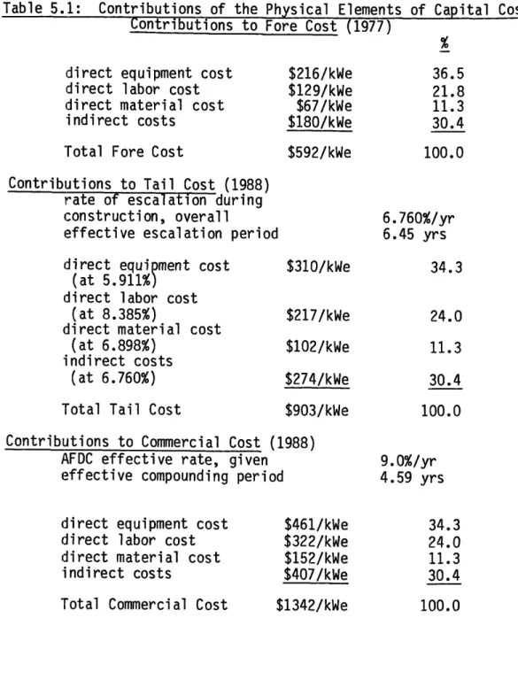
5.1 Contributions of the Physical Elements of Capital

Cost Contributions to Fore Cost 54

5.2 Capital Cost Sensitivity to Labor Requirements 64 5.3 Indirect Cost Accounts and Their Contribution to

Fore Cost 69

5.4 Sensitivity of Capital Cost to Delays and Speedups 76 5.5 Sensitivity of Capital Cost to Project Lead Time 79 5.6 Capital Cost Sensitivity to AFDC Affective Annual Rate 82 5.7 Sensitivity of Capital Cost to Project Lead Time (8% AFDC Rate) 84 5.8 Sensitivity of Capital Cost to Project Lead Time(10% AFDC Rate) 85 5.9 Contribution of the Elements of Capital Cost 89

6.1 Escalation Effects on Capital Cost 93

6.2 Effect of Escalation Rate on Capital Cost 96 6.3 Annual Escalation Rates for Some Commodities and

Services Typically Consumed in the U.S. 99

6.4 Capacity Factor Improvement Items 105

6.5 Safety-related Changes Causing LWR Plant Cost Increases

Between 1971 and 1973 108

6.6 Environmental Changes Causing LWR PLant Cost Increases

Between 1971 and 1973 111

6.7 Effect of Work Interruption on Capital Cost 117

LIST OF TABLES (continued)

Table Page

7.2 FNP Firm Price Savings 134

7.3 Multi-unit Duplicates - Schedule 140

7.4 Progress of Non-standardized Units 142

7.5 SNUPPS Plants 146

7.6 Replicate Plants Status 150

7.7 Replication Progress 150

7.8 NSSS Reference Design Status 153

7.9 NSSS Reference Design Implementation Progress 154

7.10 BOP Reference Design Status 156

7.11 Island Concept Status 159

7.12 Island Concept Implementation Progress 160

7.13 First Unit Progress with Nuclear Islands 160

7.14 LWA Progress 173

7.15 Large Utility Average Specific Cost versus Their Regional

Averages 181

7.16 UAD Financing Base Case Economic and Financial Data 205 7.17 UAD Financing Base Case - Characteristics of Power Plant

Types 206

7.18 UAD Financing Base Case - Generation Technology Mix 206 8.1 Regional Nuclear Power Plant Capital Costs 225 9.1 Historical Behavior of Fossil Plant O&M Cost 232 9.2 Contribution of FPC O&M Cost Reporting Categories

to the Total O&M Cost Value in 1975 237 9.3 LWRs Operating in 1975: O&M Cost and Number of Units

LIST OF FIGURES

Figure Page

3.1 Illustration of Capital Cost Levels 30

4.1 Average Construction Time for LWRs 44

4.2 Licensing and Time Data Summary 46

4.3 Average LWR Costs by Initial Year of Commercial

Operation 47

4.4 Estimated Commercial Costs of U.S. Nuclear Plants 49 5.1 Capital Cost Sensitivity to Labor Requirements 65 5.2 Capital Cost Sensitivity to Schedule Variations 77 5.3 Capital Cost Sensitivity to Project Lead Time 80

5.4 Effects of the AFDC Rate 83

5.5 Capital Cost Sensitivity to Project Lead Time, at 8

and 10% AFDC Rates 86

6.1 Annual Inflation Rates Since 1940 92

6.2 Effect of Escalation Rate on Capital Cost 94 6.3 Expected Variation in Labor and Material Escalation Rates 101 6.4 Qualitative Assessment of the Impact on NSSS Design of New and

Challenging Regulatory Guides, and Other Criteria 107

6.5 Percentages of Work Elements 113

7.1 Comparison of Plant Lead Times 132

7.2 Project Capital Cost Assurance 133

7.3 Licensing Lead Time for Duplicate Packages 141 7.4 Project Lead Time for First Units of Duplicate Packages 143

7.5 Gibbssar Reference Design 157

7.6 Nuclear Island Licensing Progress 161

LIST OF FIGURES (continued)

Figure Page

7.8 Reactor Vessel - Consolidated Nuclear Steam System 164 7.9 Effect of Standardization Options on Project Management 166 7.10 Standardization and Early-site Approval Effects on

Schedules 172

7.11 Comparison of Capital Cost of Plants of Large Utilities

versus Average U.S. 180

7.12 Average LWR Capital Cost by Region 182

7.13 Effect of UAD Finance on Cost of Electricity to Ultimate

Consumer 203

7.14 Electricity Cost Ratio 203

7.15 Return Requirement Sensitivity to the UAD Fraction 208 7.16 Return Requirement Sensitivity to the Gross Growth Rate 209 7.17 Return Requirement Sensitivity to the Escalation Rates 210 7.18 Return Requirement Sensitivity to the Changes in Growth

and Escalation Rates 212

7.19 Return Requirement Sensitivity to the Debt Fraction 213 7.20 Return Requirement Sensitivity to the Project Lead Time 214 7.21 Return Requirement Sensitivity with 20% Decrease in

Project Lead Time 215

9.1 Average O&M Costs by Subcategories 243

A.1 Simulation of Growth of Capacity in ULTRA Code 297 A.2 First-call Sequence of ULTRA Subprograms 311

CHAPTER I INTRODUCTION

By fall of 1976 the U.S. Energy Research and Development

Administration (now the Department of Energy) announced its concern about the future development and acceptance of Light Water Reactor (LWR) power plants in _{the United States. The ERDA concern was expressed in several} studies that were launched immediately. One of these studies is the MIT LWR Study (M3)* which was conducted during the following two years. The effort was divided among three major groups. Technical issues that affect the price of electricity produced from LWR power plants were investigated by the Technical Group. Nontechnical issues were the concern of the Institutional/Regulatory Group. Part of the effort of these two groups was to develop the appropriate input needed by the Economics Group, which was concerned with the economics of the overall U.S. electric energy supply and demand for the next two decades. The joint effort of the three groups is an examination of the large set of possible issues and alternatives that influence the future role of the LWR as a source of electricity.

The price of electric power paid by the consumer reflects the contributions of generation, transmission, and distribution. Costs of transmission and distribution are independent of the type of generating

*This indicates that the relevant information is found in reference number M3. (see the bibliography at the end of this report.)

facility. This leaves the cost of generation, or the busbar cost, as the only one sensitive to the choice of the power plant equipment.

Consideration of the factors that contribute to the busbar cost can be made by utilizing the following expression for the busbar cost, Cb:

C = [R + 0 + F (1.1)

where

K = capacity factor, actual kWehr/rated kWehr,

R + 0 = fixed (capital plus operating) cost, mills/kWehr, and F = fuel cycle cost, mills/kWehr.

One section of the Technical Group working on this project was involved in _{studies of the capacity factor. Another section examined the fuel} cycle cost. The work presented in this fixed cost assessment report is the contribution of the third technical section. Parallel to other

activities associated with the overall project, the Fixed Cost Assessment Section investigated the fixed cost status, current trend, the factors contributing to this trend, assessment of possible improvement

alternatives, and the factors that limit the range of improvement. As shown above, the fixed cost is the sum of two terms. The first term, R, represents the return requirement on capital investment. This investment is _{associated with the total cost of building the nuclear power plant and} placing it _{into commercial operation. The value of R represents both} direct and indirect costs. Direct costs are those associated on an item-by-item basis with land and land rights, the physical plant

(structures, equipment, and materials), and the labor involved. Indirect costs include expenses for services such as engineering and design,

construction facilities, taxes, insurance, and interest during

construction, and general items such as staff training, plant start-up, and general and administrative overhead of the owner. The first core loading investment cost is not included in the capital cost; it is considered part of the fuel cost.

The second term, 0, represents the operation and maintenance

charges. It includes the operating costs of plant staffing and nuclear liability insurance. Maintenance costs include coolant/moderator makeup, consumable supplies and equipment, and outside support services. In addition to these major items, there are miscellaneous O&M costs associated with staff replacement, operator requalification, annual

operating fees, travel and office supplies, the owner's other general and administrative costs, as well as working capital requirements.

The cost of plant backfitting due to evolving safety and

environmental regulations and, to a lesser extent, due to enhancing plant performance, is of a capital cost nature, but in some cases it has been included in O&M costs. As we will see later, some utilities find it expedient to expense the backfit costs rather than capitalizing them. With the preceding discussion in mind, one can see that the fixed cost components are no longer fixed with time. The adjective "fixed" indicates that the relevant cost is independent of the quantity of power generated. This is true for the capital cost term and the operation part of the second term. Although the cost associated with the maintenance

activities is highly variable in theory, it is practically confined, on the average, to a narrow range for any given power plant. Because the

fuel charges are variable, theoretically or otherwise, and for the lack of a better term, all the non-fuel charges have been called Fixed Cost.

In 1977, a typical set of figures related to the details of the busbar cost is as follows (El):

capital investments $764/kWe fixed operation cost $2.62/kWe yr variable maintenance cost $0.66/MWehr fuel cycle cost (1977) $0.53/MBtu

Assuming 65% as the value for the capacity factor and 18% for the

levelized annual fixed charge rate, the following table can be produced

capital return requirement O&M charges fuel charges Busbar cost mills/kWehr % 24.15 78.95 1.12 3.66 5.32 17.39 30.59 100.00

The various sources described in Chapter II report the following ranges: capital return requirement 68-80%

O&M charges up to 10%

The fuel charges take the balance of the busbar cost.

The aim of this discussion is to assess the relative importance of each of the two (fixed cost) components. It is apparent that the capital cost carries almost all the fixed cost weight. It turns out that because of the nature of the activities involved in constructing and operating such projects, capital cost is more controllable. This is because the

number of key people involved in the construction stage is limited

relative to that in the O&M stage; the expenditures are much larger, and therefore more cautious planning is attainable. In the case of operation and maintenance cost, every power plant has its own team, the

expenditures are relatively low, and decisions are more of a reactionary type, reflecting instantaneous circumstances.

Because more attention has been paid to capital cost in the

literature (as indicated in the later chapters) compared to the several detailed studies that were done related to capital cost, so the author encountered only one short, and in some sense incomplete, study of O&M cost (Al). In any case, the relative importance led, at an early stage of this work, to the decision to concentrate most of the effort on the treatment of the capital cost. In this report, topics related to the discussion of the two components (R and 0) are tested in a parallel fashion wherever possible.

Work on this study has involved extensive literature search,

utilization of computer codes (both available and newly developed), and assessment of data obtained by surveying the U.S. nuclear industry and utilities. This report consists of ten chapters and an appendix. The following chapter deals with survey data. It offers a background for the motivations that guided the rest of the report. The next six chapters reflect the bulk of the study in the area of capital cost assessment. Chapter III discusses capital cost estimation and the base case. Chapter

IV presents the trend of capital cost. Chapter V investigates the

of capital cost behavior. These four chapters lay the background for the major goal of this study, which is the to assess the possible

alternatives for capital cost improvement presented in Chapter VII. The factors that may limit such improvement are presented in Chapter VIII. Assessment of the other fixed cost component, the operation and

maintenance cost, is presented in Chapter IX. The flow of material in Chapter IX is parallel to that of Chapters III through VIII. The last chapter gives a summarizes the report and discusses recommendations for future work.

Throughout this study, sources of data other than the survey are utilized, as indicated and cited in the text. When data samples are used, no statistical effort is made beyond evaluating the mean value and the standard deviation in order to identify the data spread. More

sophisticated steps can be used to assess the data. Such effort, however, is sacrificed to give attention to more profound issues.

Unlike several other studies, especially in the capital cost area, the main objective of this part of the MIT LWR Study is not merely to assess the current status of LWR fixed cost, its trend, and the causes of this trend. This study addresses, for the first time, the different

fixed cost improvement strategies, their effectiveness as based on analytical and historical evidence, and the limiting factors that may impede such improvement. In Chapter VII three sets of possible

improvement alternatives are investigated. Most of these alternatives have been proposed and exercised for a period of time. In order to reach a comprehensive improvement strategy this report proposes improvement in

two additional areas: periodic regulatory freezes and financing. The latter received more attention. A computer code to investigate the Ultra-accelerated Depreciation financing has been developed and is shown in the appendix.

As presented in Chapters III through VI, LWR capital cost involves a large amount of funds to be spent over a long period of time before

economically produced electricity is generated. LWR project lead times have become longer than the conventional planning horizons of electric utilities. Capital investment has become too large for many utilities to procure the necessary funds, internally or externally. This means that, while LWRs remain economically attractive as electricity sources, as shown by the output of the Economics Group, they tend to price themselves out of the market. This situation is shared by all new or improved

technologies, such as the breeder reactor, whose capital cost is estimated to be 50% higher than that of LWRs (S5), future fusion machines, and even current coal-fired plants whose capital cost is catching up with LWRs. Therefore, a comprehensive strategy for capital cost improvement is the major objective of this study. The aim is to

improve the electricity busbar cost. This can be done by improving capital cost in a controllable way that does not allow for undesirable changes in other busbar cost components to dominate.

It is important to remember that the capital cost assessment in this study is a technical study made primarily for the purpose of assessing the relative sensitivity to various options. The absolute capital cost values are derived to be reasonable but are not the primary goal of the

study. This study is only concerned with matters relevant to the technological, environmental, financial, and managerial aspects

determining nuclear power plant capital investment. The study therefore concentrates on areas that are important as input to the "global system" economic sensitivity studies.

CHAP TER II

ASSESSMENT OF U.S. SURVEY DATA

This study is concerned with the assessment of the various

strategies that the U.S. Department of Energy may pursue or assist in implementing, to improve the Light Water Reactor power plant industry's current status and future trend from the vantage point of fixed costs. The span was taken to be 20 years, i.e. 1977 to 1997. As the problem was formulated and the means of solution were sketched, a number of unknowns were identified. These unknowns are called variables. Each of these variables was expected to have a range of possible values, the choice of which depends on relevant conditions.

The lack of sufficient and up-to-date information in the literature made it _{necessary to survey of the nuclear industry to develop a data} base for this study. In addition, the nuclear industry is the most

sensitive sector of the society to the outcome of the study and obviously the opinion and judgment of those in the industry are the most

knowledgeable on related matters. Hence their assistance was solicited in evaluating the variables and also in carrying out the overall study. The survey was made in the form of a numerical questionnaire, with provision for comments in some specified areas. The text of the

questionnaire included a defined list of variables, answer sheets, and instructions. The variables were divided into groups, according to the specialty and experience of the information source, with some overlap

between groups. Consequently the answer sheets were designed according to the groups of variables and the related assumptions. These

assumptions correspond to the different alternatives that may be

considered for improving each of the components of the fixed cost. The list of variables and assumptions was made as comprehensive as possible, and by no means was it expected to be fully completed by any one of the information sources. The list of information sources consisted of directly-contacted and indirectly-contacted members of the nuclear industry. The first category is composed of 14 companies. Their specialities are as follows:

Equipment vendors 3

Architect/Engineer-constructor 2

Research group 1

Utilities 8

With members of this group we had personal contacts involving one or more meetings, as well as other forms of communication. The group of

variables for which information was requested of the A/E firms and the utilities was large. Hence it had to be broken down into four subgroups when contacts with a second category of information sources were made. This category includes 24 utilities and one architect/engineering firm. About one-third of the 38 sources have provided us with complete positive

responses. All information sources were given anonymity. All

information obtained from any of them will be referenced as "our survey sources."

2.1 Data from the Survey of U.S. Nuclear Industry

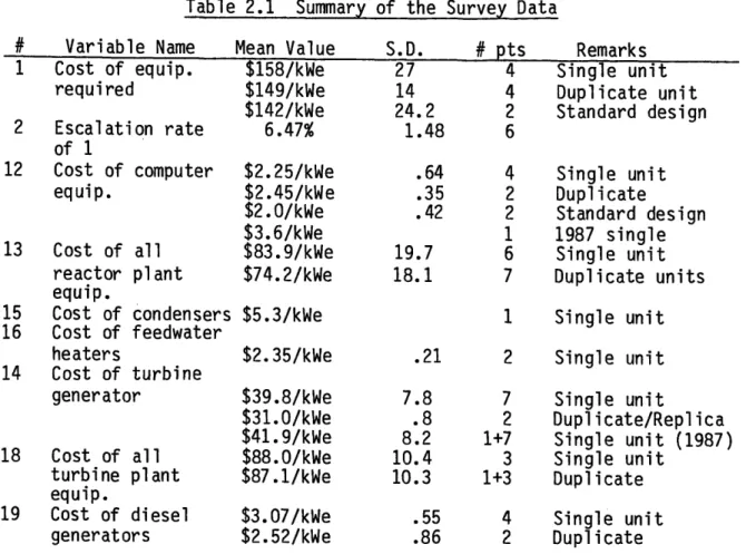
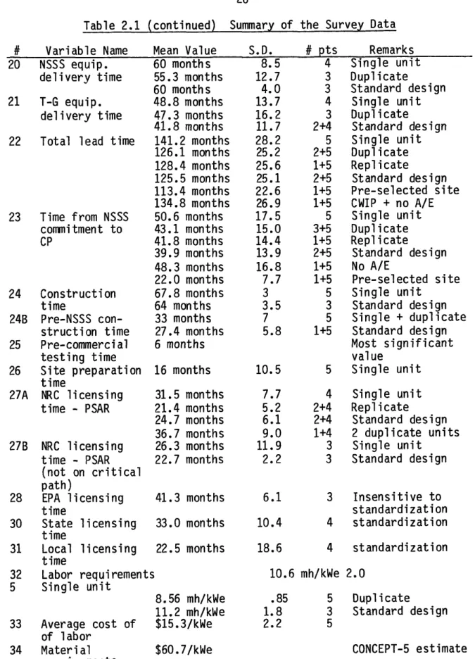
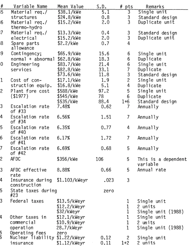
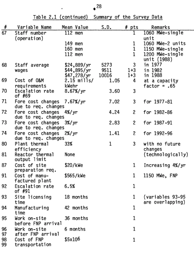
The results of the survey data are presented in Table 2.1. The first column on the left has the serial numbers with which the variables are located on the list of variables. The second column gives a brief description of the variable. The next two columns give the mean value and the standard deviation of the data, using the same units. The fifth column gives the number of points (information sources) from which

pertinent data were obtained. The last column describes the assumptions associated with the adjacent value assigned to the variable. All data reflect 1977 conditions unless otherwise stated. SINGLE UNIT means that the plant has one unit, designed, licensed, and constructed without taking advantages of standardization. DUPLICATION means that more than one identical units are considered, with one or more utilities building and licensing them, or more than one unit in operation under the same management at the same site. STANDARD DESIGN is when a combination of Reference Systems for the Nuclear Steam Supply System and Balance of Plant is exploited (see Section 7.2). REPLICATION is similar to DUPLICATION except the licensing effort of the latter unit is separate from that of the referenced unit. CWIP is when the Construction Work in Progress is added to the current rate base, and hence the allowance for funds using during construction is billed directly to current consumers. NO A/E means that the utility does its own architect/engineering and construction activity with no outside support in these areas.

PRESELECTED SITE reflects the condition when the necessary activities for site selection are completed prior to NSSS purchase. Other remarks are

self-explained. _{Information that reflects the possible implementation of} other assumptions (or conditions) as well as the majority of the future projections could not be obtained. Some of the collected data reflected a misunderstanding of the relevant questions or use of alternative

definitions that resulted in inconsistencies. These data were not included in the statistics. Some sources gave information on some variables under some assumption such that when compared with other data from a different set of sources concerning the same variable, results were distorted. This can be noticed in a few cases in the table. When major distortions or inconsistencies were observed, the method of calculating the mean and the standard deviation is altered. This is found wherever the number of points is expressed as n + m. m is the number of points used to generate the first value reported for the

variable, while n is the number of points that are shared consistently by the two sets of assumptions. As an example, consider variable 22. The figure 141.2 + 28.2 is based on m = 5 data points. The next value 126.1 + 25.2 is based on 2 + 5 data points. m = 5 are the same data points used for the first value. When the second value was calculated there were more than two data points under the duplicate assumptions. Only 2 points are consistent with the set of 5 points used to calculate the single unit value. When these 2 points are compared with their

counterparts in _{the 5-point set, the value 141.2 + 28.2 was scaled down} to 126.1 + 25.2. Comparison is carried out between sets of data that are obtained from the same set of information sources.

The data presented in _{Table 2.1 form the basis for the analyses} presented in _{the remainder of this report. Examples are the set of input}

data for CONCEPT code calculation of the capital cost base case estimate in _{Chapter III, variations of capital cost base elements in Chapter V,} and O&M cost related data in Chapter IX. In Section 6.1, Table 2.1 data helped to assess the effects of escalation, and to assess standardization in _{Section 7.2. The assistance of the survey data in Chapter IV was} limited, since only a small set of future-related data extending to the late 1980s was obtained. Our survey sources indicate that uncertainties for future projections are too high to generate dependable data.

Therefore, the use of these data for future projections must be

considered as highly uncertain beyond 1990, and the work discussed here is limited to a time span up to 1990.

Table 2.1 Summary of the Survey Data # Variable Name 1 Cost of equip. required 2 Escalation rate of 1 12 Cost of computer equip. 13 Cost of all reactor plant equip. 15 Cost of condensers 16 Cost of feedwater heaters 14 Cost of turbine generator 18 Cost of all turbine plant equip. 19 Cost of diesel generators Mean Value $158/kWe $149/kWe $142/kWe 6.47% $2.25/kWe $2.45/kWe $2.0/kWe $3.6/kWe $83.9/kWe $74.2/kWe $5.3/kWe $2.35/kWe $39.8/kWe $31.0/kWe $41.9/kWe $88.0/kWe $87.1/kWe $3.07/kWe $2.52/kWe S.D. 27 14 24.2 1.48 .64 .35 .42 19.7 18.1 .21 7.8 .8 8.2 10.4 10.3 .55 .86 # pts 4 4 2 6 4 2 2 1 6 7 1 2 7 2 1+7 3 1+3 4 2 Remarks Single unit Duplicate unit Standard design Single unit Duplicate Standard design 1987 single Single unit Duplicate units Single unit Single unit Single unit Duplicate/Replica Single unit (1987) Single unit Duplicate Single unit Duplicate

Table 2.1 (continued) Summary of the Survey Data # Variable Name b 20 NSSS equip. delivery time 21 T-G equip. delivery time 22 Total lead time

23 Time from NSSS commitment to CP 24 Construction time 24B Pre-NSSS con-struction time 25 Pre-commercial testing time 26 Site preparation time 27A NRC licensing time - PSAR 27B NRC licensing time - PSAR (not on critical path) 28 EPA licensing time 30 State licensing time 31 Local licensing time 32 Labor requirements 5 Single unit 33 Average cost of of labor 34 Material requirements Mean Value 60 months 55.3 months 60 months 48.8 months 47.3 months 41.8 months 141.2 months 126.1 months 128.4 months 125.5 months 113.4 months 134.8 months 50.6 months 43.1 months 41.8 months 39.9 months 48.3 months 22.0 months 67.8 months 64 months 33 months 27.4 months 6 months 16 months 31.5 months 21.4 months 24.7 months 36.7 months 26.3 months 22.7 months 41.3 months 33.0 months 22.5 months S.D. 8.5 12.7 4.0 13.7 16.2 11.7 28.2 25.2 25.6 25.1 22.6 26.9 17.5 15.0 14.4 13.9 16.8 7.7 3 3.5 7 5.8 10.5 7.7 5.2 6.1 9.0 11.9 2.2 6.1 10.4 18.6 # pts 4 3 3 4 3 2+4 5 2+5 1+5 2+5 1+5 1+5 5 3+5 1+5 2+5 1+5 1+5 5 3 5 1+5 Remarks Single unit Duplicate Standard design Single unit Duplicate Standard design Single unit Duplicate Replicate Standard design Pre-selected site CWIP + no A/E Single unit Duplicate Replicate Standard design No A/E Pre-selected site Single unit Standard design Single + duplicate Standard design Most significant value 5 Single unit 4 2+4 2+4 1+4 3 3 Single unit Replicate Standard design 2 duplicate units Single unit Standard design 3 Insensitive to standardization 4 standardization 4 standardization 10.6 mh/kWe 2.0 8.56 mh/kWe 11.2 mh/kWe $15.3/kWe $60.7/kWe .85 1.8 2.2 5 3 5 Duplicate Standard design CONCEPT-5 estimate

Table 2.1 (continued) Summary of the Survey Data # Variable Name 35 Material req./ structures 36 Material req./ thermo-hydro 37 Material req./ electrical 38 Spare parts allowance 39 Contingency; normal + abnormal 40 Engineering services 41 Cost of con-struction equip. 42 Plant fore cost

($1977) 43 Escalation rate of #33 44 Escalation rate of #34 45 Escalation rate of #40 46 Escalation rate of #41 47 Escalation rate of #42 52 AFDC 53 AFDC effective rate 54 Insurance during construction

55 State taxes during #23 63 Federal taxes 64 Other taxes in commercial Mean Value $38.1/kWe $24.8/kWe $15.2/kWe $13.3/kWe $15.2/kWe $2.2/kWe $65.9/kWe $62.8/kWe $83.7/kWe $82.8/kWe $73.6/kWe $17.1/kWe $16.8/kWe $588/kWe $545/kWe $535/kWe 7.48% 6.56% 6.35% 6.17% 6.69% $356/kWe 8.88% $1.103/kWeyr S.D. 5.1 0.8 2.0 0.4 2.0 0.7 15.6 18.3 21.4 33.1 11.8 1.9 5.1 97.2 78 88.4 0.62 1.51 0.77 1.72 0.68 106 0.66 .023 # pts 3 3 3 3 3 4 Remarks Single unit Standard design Duplicate unit Standard design Duplicate unit 6 Single unit 6 Duplicate 6 Single unit 7 Duplicate 3 Standard design 2 Single unit 4 Duplicate 5 Single unit 6 Duplicate 1+6 Standard design 7 Annually 7 Annually 4 Annually 7 Annually 5 Annually 5 This is a dependent variable 5 Annual rate 3 zero $13.5/kWeyr $12.2/kWeyr $32/kWeyr $12.1/kWeyr $10.9/kWeyr operation 28.7/kWeyr 65 Operating fees zero

66 Nuclear iability $1.22/kWeyr insurance $1.12/kWeyr 1 Single unit 1 2 units 1 Single unit 1 Single unit 1 2 units 1 Single unit 0.12 0.11 (1988) (1988) 2 Single unit 1+2 2 units

---Table 2.1 (continued) Summary of the Survey Data # Variable Name 67 Staff number (operation) 68 Staff average wages Mean Value 112 men S.D. 149 men 160 men 112 men $24,889/yr $44,895/yr $47,278/yr 69 Cost of O&M 2.15 mill

requirements kWehr 70 Escalation rate 8.67%/yr

of #69

71 Fore cost changes 7.67%/yr due to req. changes

72 Fore cost changes 4%/yr due to req. changes 73 Fore cost changes 3%/yr

due to req. changes 74 Fore cost changes 2%/yr

due to req. changes 80 Plant thermal 33%

efficiency

81 Reactor thermal None output limit

87 Cost of site $20/kWe preparation req.

91 Cost of manu- $565/kWe factured plant

92 Escalation rate 6.5% of #91

93 Site licensing 18 months time

94 Manufacturing 42 months time

95 Work on-site 36 months before FNP arrival

96 Work on-site 6 months 97 after FNP arrival 98 Cost of FNP $5x106 99 transportation s/ 5273 9511 10016 1.05 3.60 7.02 4.24 2.83 1.41 1 # pts Remarks 1 1060 MWe-single unit 1 1060 MWe-2 units 1 1150 MWe-single 1 1200 MWe-single unit (1988) 3 in 1977 1+3 in 1982 1+3 in 1988 4 at a capacity factor = .65 3 3 for 1977-81 2 for 1982-86 2 for 1987-91 2 for 1992-96 3 with no future changes (technologically) 1 Increasing 4%/yr 1 1150 MWe, FNP 1 1 (variables 93-95 are overlapping) 1 1 1 1

C H A P T E R III CAPITAL COST ESTIMATE

This chapter covers the area of capital cost estimate. It starts with establishing some basic definitions to be used for the remainder of the report, then reviews the capital cost estimates and calculations, and concludes with establishing the base case.

3.1 Basic Definitions

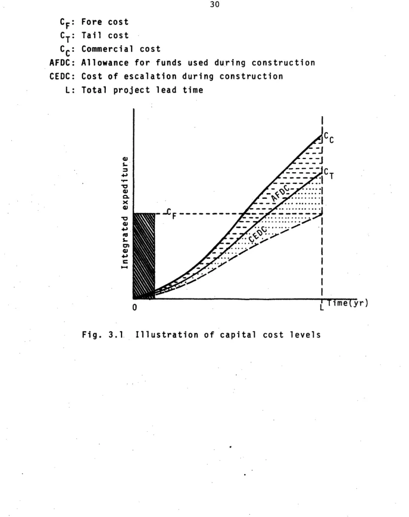
In _{order to provide a consistent set of terms, the following} definitions are made and clarified by Figure 3.1.

1) The Fore Cost. This is the cost of all equipment, materials, and services that will be consumed until the completion

of the project, evaluated in terms of the prevailing prices at the beginning of the project. Hence the fore cost is given in dollars valued at about the time the decision to purchase is being made.

2) The Tail Cost. This is the cost of equipment, materials, and services that will be consumed during the completion of the project in terms of prices that are actually (or expected to be) paid at the time of their purchase, according to the then-market conditions, throughout the construction period. Note that the fore cost and the tail cost account for the same

items of equipment, labor, materials, and services.

CF: Fore cost CT: Tail cost

Cc: Commercial cost

AFDC: Allowance for funds used during construction CEDC: Cost of escalation during construction

L: Total project lead time

.

XH-

:.I

Li

Fig. 3.1 Illustration of capital cost levels

aJ 0. x (g 4) M . 4.) 4)

4-PI;S,

;O;-

I

cost and the fore cost. It may be referred to by CEDC for the cost of escalation during construction.

4) Allowance for Funds used During Construction, AFDC. This is the cost of investment during the construction period. It is the sum of the interest on the borrowed fraction of capital, and the opportunity cost on the equity part.

5) The Commercial Cost. It is the tail cost added to the

associated AFDC. It thus represents the total project cost for the utility, including their opportunity cost of investment. Alternatively, this is the book value of the plant at the start

of commercial operation. The rate base of electricity is made considering the commercial cost.

The contribution of the capital cost to the busbar cost is given by the value of the commercial cost, CC, as the plant goes into commercial operation. This set of definitions describes "levels" and components of capital cost. These "levels" are the fore cost, CF, the tail cost,

CT, and the commercial cost, CC. They have the following relationship:

CC(t) = CF(t - L) +CEDC(L) + AFDC(L) (3.1)

= CT(t) + AFDC(L) (3.2)

where

L = project lead time, years t = calendar time, years

CEDC = cost of escalation during construction, and AFDC = allowance for funds used during construction. It is interesting to clarify the preceding definitions by a

numerical example. In Section 3.3 the fore cost is calculated for a special case as $592/kWe for 1977. Eleven years later, the CEDC was $312/kWe, making the tail cost $903/kWe. The AFDC during the same period was $438/kWe, and the commercial cost was $1342/kWe.

The same computational procedure was repeated, assuming historically averaged values of 7% AFDC annual rate, 9 years for project lead time, and 3 years for construction permit lead time. The same reactor size was used and the date of commercial operation was January 1, 1977. The

resulting commercial cost value is $599/kWe, which is only 1% higher than the first value. These two values are in good agreement when the

uncertainties in determining the computational parameters are

considered. The obvious conclusion is that the fore cost of a given plant at any point in time is the same as the commercial cost of a similar plant that has just been completed under similar project

conditions. Based on historical economic data since 1953, a recent study concludes that the fore cost is + 6% of commercial cost of the same

date. On the average, CF is only 1% higher than the CC (J1).

3.2 Use of CONCEPT Code, Phase 5

The CONCEPT code is a package of three computer programs that were developed at Oak Ridge National Laboratory and the Computing Technology Center (E2). It consists of a main program, CONCEPT, that accepts as

input for each run, information about size, location, and type of plant, as well as the dates associated with NSSS commitment, issue of

as a source of information and a means of comparison wherever possible in this study.

To carry out the necessary calculations, CONCEPT utilizes the output of the two other programs. CONTAC generates data files for the various types of plants from the relevant cost models. The words "type of plant" refer to whether it is, say, coal-fired with scrubbers, whether it is a first or second unit, and the kind of cooling system employed. The expression "cost model" means the item-by-item detailed description of plant equipment, necessary material and labor to build the plant and install equipment in place, and the associated costs. The CONLAM program reads historical data for labor and material costs for each of 23

locations in the U.S. and Canada, and generates data files to be used by CONCEPT.

Any changes in the cost models for any of the various types of plants result in another run of CONTAC program to produce a new data file for CONCEPT. The same is true with respect to labor and/or material

related changes and the CONLAM program. Minor changes, however, can be temporarily implemented during the use of CONCEPT without altering the relevant data files. To appreciate this arrangement, we notice that a CONLAM run on the MIT computer system costs about $45 and a CONTAC run

costs about $95. These preliminary runs result in about $2.50 for each CONCEPT run during normal usage. On the other hand, using raw data for the CONCEPT program may result in a cost of $8.00 per run.

The package is continuously undergoing development and updating. At MIT we first obtained the CONCEPT Phase 4, Code package (CONSYS4). This

is the most informative and flexible version of the code. It has equipment price data for June 30, 1975, and labor and material data relating to the beginning of 1977. The drawback of this package is that it still uses cost models created in 1972 (W1). This causes the code estimates to be lower than actual ones made by utilities and vendors.

The Phase 4 code was used in the early stages of the study and its output was normalized against updated data. Later, an early edition of CONCEPT code, Phase 5 was obtained (H2.) It has computational features similar to those of Phase 4. More detailed output can be generated. It still follows the accounting system presented in the USAEC Code of

Accounts (N1) in an expanded form as compared to Phase 4. The main advantage in this phase of CONCEPT code is the newly updated cost models which are based on the latest United Engineers and Constructors Study

(N2) and were modified as late as June 1977. The labor and materials data were modified by the same date. Unlike CONCEPT-4, CONCEPT-5 has only the LWR and coal-fired power plants options. These two types of

large power plant technologies are the ones mostly expected to be utilized in the foreseeable future. Because work on CONCEPT-5 has not been completed by the time we obtained the said edition, the only option of cooling system available was that of mechanical draft cooling towers. This has restricted our flexibility in this relatively minor area (see Section 3.3).

Few changes were needed in the program sources in order to make them operable on the MIT computer facility. The changes included modifying the subroutine IDAY encountered in CONCEPT-4 and CONTAC-4, and

programming changes in CONLAM-4 to make it read input data from the

magnetic tape prepared at ORNL. In the CONCEPT-5 package, only the first change had to be implemented.

3.2.1 Accuracy of CONCEPT Code, Phase 5

There have been two instances where actual data have been obtained (from our survey sources) as a complete set usable for CONCEPT-5 input. These data were accompanied by actual cost estimates of the relevant power plants. The following presents the important points of comparison between CONCEPT-5 calculations and actual detailed estimates made by utilities.

Case 1: one unit plant

Commercial Cost (1985)

$/kWe %

Actual Estimate 1525 100.00

CONCEPT-5 Calculation 1187 77.85

Case 2: 2 unit plant total estimates

Labor Require- Tail Cost

ments (1985)

Manyears % $/kWe %

Actual Estimates 11, 500 1T 1650 100

CONCEPT-5 Calculation 10,448 90.85 1537 93.15

In both cases the Code has underestimated the actual figures. The first case project started relatively early and licensing delays and

conditions. CONCEPT estimates are within 9% of the utility estimates in Case 2, a reasonably good agreement in this case.

3.3 The Capital Cost Base Case

A base case data set had to be established as a prerequisite to further analyses. In addition, the base case was needed for the MIT Regional Electricity Supply Model (REM), which is used by the Economics Group to do overall cost-benefit evaluations of alternative LWR

improvement strategies. As an input to REM, fore cost data are required for typical generating plants. Allowance has been made for the base case for the coal-fired plants (with fewer details) in addition to that of the LWR power plants.

3.3.1 Capital Cost of LWRs

Any power plant construction project is characterized by equipment, labor, material, and time requirements. The base case parameters are those that determine the base case capital cost value. With the assistance of the data presented in Chapter II, these parameters have been determined, then used as the standard input into CONCEPT code, Phase 5. The base case parameters are as follows:

a) Plant Power Capacity

The most popular size of generating units among the sources we contacted is 1150 MWe. There were 59 generating units that have been applied for to the NRC (AEC) between Jan. 1, 1974 and the end of 1975 (N3). The mean size of these reactors is 1181 MWe, with a standard deviation of 120 MWe. When two 900 MWe units and two 906 MWe units are

taken out, a sample of 55 reactors remains. The lowest reactor size in this sample is 930 MWe. The average size of the 55 reactors is 1201 MWe with 96 MWe as a standard deviation. Note that in this sample, except for four reactors that are of 930 MWe, all other sizes start from 1120 MWe. This sample reflects the notion of the industry about the optimum future reactor generating capacities. Hence, for convenience and

consistency, the plant size was taken as 1200 MWe. b) Reactor type

Only 14 of these reactors were of the BWR type. Forty-one reactors are of the PWR type. Four others were undecided (and were canceled 4 years later). This makes the PWR/BWR ratio 3 to 1. Investigation of

additional information (N2) shows that the two types of power plants come close within 2% of fore cost. The base case reactor type was arbitrarily chosen to be a PWR. Table 3.1 shows results of CONCEPT-5 calculations.

Table 3.1 Cost Comparison of Reactor Types (CONCEPT-5 Output)

LABOR REQ'MT FORE COST TAIL COST COMMERCIAL

REACTOR TYPE (1977) (1988) COST (1988)

manhours/kWe % $/kWe % $/kWe % $/kWe % PWR (base 9.282 100.00 592 100.00 903 100 1342 100.00

case)

BWR 9.497 102.32 591 99.83 903 100 1340 99.85

c) Number of units per plant

Although many sites have, or are planned to have, more than one unit per plant, one unit per plant was chosen. This is because there are many

cases where the reactor is truly a first unit, and many others where the advantage of being a second duplicate unit could not be taken.

d) Cooling system

The type of cooling system for the plants described in a) above, was distributed as follows:

Once-through cooling 11 units Natural draft towers 21 units Mechanical draft towers 23 units.

The third type of cooling system was chosen because of the restrictions of the available version of CONCEPT-5. CONCEPT-4

calculations for the three cooling systems are made with the same base case input data. The results are shown in Table 3.2. The cost

comparison between the three types of cooling systems shows that the choice of mechanical draft cooling towers is an acceptable assumption.

Table 3.2 Cost Comparison of the Cooling Systems (CONCEPT-4 Output) LABOR REQ'MT FORE COST TAIL COST COMMERCIAL

TYPE OF (1977) (1988) COST (1988)

COOLING

SYSTEM manhours/kWe % $/kWe % $/kWe % $/kWe % Mechanical Draft 7.745 100.0 401 100.00 636 100 946 100.0 Natural Draft 7.983 103.1 407 101.5 644 101.3 958 101.3 Once-through 8.142 105.1 407 101.5 649 102.0 967 102.2 e) Location

project working groups. This location has the following features: 1) It is a real location.

2) It is very close to the conditions in terms of final cost data of the hypothetical site, Middletown, USA used in CONCEPT

code-related studies as the reference site.

3) Although the Northeast region is the worst region from fixed cost considerations as shown by the EPRI study (El), nuclear energy stands as the major electricity source beside oil in this region. The EPRI study shows that this region has the highest capital cost--about 10% larger than the average over all U.S. regions (see Table 8.1 in Chapter VII).

f) Date of NSSS Commitment

January 1, 1977 is taken as the reference date for fore cost data. g) Date of Construction Permit

Table 2.1 shows a construction permit lead time (variable 23) of 50.6 + 17.5 months for single unit plants. It shows lower values for other special cases. Forty-eight months is taken as the convenient value. Hence, the CP date is January 1, 1981.

h) Date of Commercial Operation

Table 2.1 shows the total project lead time (variable 22) as 141.2 + 28.2 months, or a mean value of 11.75 years for single unit plants. It shows much shorter times for other alternatives. Eleven years is chosen and the commercial operating date is January 1, 1988.

i) AFDC Effective Annual Rate

The value of 8.48 + 1.05% is shown in Table 2.1 (variable 53) for the AFDC. As a convenient conservative value, recommended by some industry sources, 9.0% was chosen.

The last three parameters, g, h, and i, do not affect the fore cost value. Other important parameters, such as the costs of equipment and materials, and labor requirements, were left to be calculated by the code. The values for these parameters, as calculated by the code, were different from those shown in Table 2.1 in an inconsistent manner.

Consequently, the code-computed values for these parameters were left as a part of the base case value, and Table 2.1 data are reserved as a guide for the sensitivity studies. The results of CONCEPT-5 calculations are

summarized in Table 3.3. Note the remarkably close agreement between the CONCEPT-5 value for the 1977 fore cost and that reported in Table 2.1

(variable 42).

Table 3.3 LWR Base Case Capital Cost Fore Cost (1977)

Total

direct equipment cost direct labor cost direct material cost indirect costs

contingency allowance (at 10%) Labor requirements Tail Cost (1988)

rate of escalation during construction overall

equipment labor material

cost of escalation during construction total tail cost

AFDC (1977-1988)

AFDC effective annual rate, given AFDC Commercial Cost (1988) $592/kWe $196/kWe $117/kWe $61/kWe $164/kWe $53/kWe 9.282 manhours/kWe 6.760 %/yr 5.911 %/yr 8.385 %/yr 6.898 %/yr $312/kWe $903/kWe 9% $438/kWe $1342/kWe

The 1977 fore cost figure was passed to the Economics Group for use as input to the REM code.

3.3.2 Capital Cost of Coal-fired Plants

Upon request from the Economics Group, the 1977 fore cost value for a typical coal-fired plant was estimated. The values of the base case parameters that affect the fore cost are the same as those for the LWR plants, except for the following:

a) Plant Power Capacity

As recommended by some industry sources, the optimum size for coal-fired plants is around 800 MWe. This is determined by the

construction and the operation and maintenance economics. These in turn are consequences of the nature of the fuel as well as the

state-of-the-art. CONCEPT-5 references a plant of 794 MWe capacity, and this value was taken for this parameter.

b) Equipment

The plant is a coal-fired unit with a flue-gas desulfurization system (scrubbers). This is expected to be the prevailing design for future plants due to environmental restraints.

The result of the base case calculation is: Total Fore Cost (1977) $515/kWe. 3.3.3 Assessment of the Base Case Data

Section 3.2.1 shows that CONCEPT-5 calculations deviate within about 9% of utility estimates for an ongoing nuclear power plant project

Section 3.2.1 results also tend to confirm Table 2.1, as it will be seen in several cases. In other cases Table 2.1 data have some defects that will be discussed later. The 9% deviation is not so large that

improvement on Table 3.3 becomes necessary. The $1.61 billion figure for the 1988 commercial cost is in close agreement with other estimates. In fact both fore cost and commercial cost figures seem higher than the

national averages presented in the next chapter. Finally, the main role of the base case is to examine the impact of varying the relevant

CHAPTER IV PRESENT TREND OF CAPITAL COST

The present day status of LWR capital cost is described by the base case data set. The 1977 fore cost is $592/kWe. This has increased from $211/kWe in about 4-1/2 years (W1). Table 2.1 shows that the same value (variable 42) should be $588 + 97.2/kWe. The mean value is statistically undistinguishable from the base case value. The 16.5% standard deviation may be explained by regional variations, as discussed later in Section

8.2.

Eq. 3.1 expresses the commercial cost as the sum of the fore cost, the CEDC and AFDC. Since the main determinant of the CEDC and AFDC is the fore cost itself, this makes the commercial cost strongly dependent on the behavior of the fore cost. The average annual rate of increase of the fore cost over the last 4-1/2 year period, from $211/kWe to $592/kWe, is 25.8%.

The other factor that influences the commercial cost is the project lead time. This has changed dramatically over the past decade. Figure 4.1 shows the average actual construction time of LWRs for the period 1969-1977, and the estimated construction time for years beyond 1977. Parallel to the fore cost changes, the construction time (about 60 to 75% of project lead time) was 66 months for plants completed in 1972 and between 90 to 105 months for plants completed in the 1976-78 period. It is observed that for plants completed in the 1970s, the construction

- 0) sauow J uloo (p u! 'u o cJn

S44UOW JDPUOID u uoioinf

O o o a, c' C, 0) C0j 0 a, C) -E _₀ E (O O 0 0 -C: O) o CU PC C C~J -E _o s o

time increased about 4 months/year (M1). The overall increase in the five-year (1972-77) period is about 50% for the construction time.

The CP lead time (time to obtain the Construction Permit) exhibits similar behavior, as seen in Figure 4.2. For the 1966-71 period the CP lead time increased at a rate of 5 months/year (M1). Figure 4.2 shows that 3.5 out of the 5 months/year increase is in the period of

Preliminary Safety Analysis Report (PSAR) review. This makes the project lead times for plants to be completed in the 1970s increase at a rate of 9 to 10 months/year. Even though attempts to improve the licensing

procedures are being made so this trend is not expected to hold for the Eighties, it is not inconceivable that further increases will occur due to unforeseen factors.

The consequences on commercial cost are pronounced. Early in the last chapter we saw the relationship between the fore cost and the

commercial cost. While the 1977 commercial cost (the 1977 fore cost for plants considered in 1977) is estimated at $592/MWe, the commercial cost for the same plants in 1988 is $1342/kWe (see Table 3.3). This

corresponds to a 127% increase in 11 years, or an annual average of 7.74%. Figure 4.3 supports this estimate. The data in this figure start with $534/kWe for 1977 and end with estimated commercial cost of

$1062/kWe for 1987. On the other hand, it shows about $450/kWe for large units in 1977. This is about 24% lower than the base case value, which is for a plant in the same category. Note that only two LWR units

contribute to this low figure. This large discrepancy is due to the fact that the base case calculation was done for the Northeast region, which

(D

0 0 0 0 0 0

O O 04 OJ O

(sqluouJ) d3 ol lae)op uoJe atoll

r,-N. _U L c E - c b. o C 0)0 _{O D} u - ' -_0

0 0 0 0 0 0 0 o ¢

0 0 0 0 0 0 0

0--- 0 O P - w In

IOU M)I/ 'ISo I!dDo 4!Ufn

(D _C -I .2

u

is _{of a very high cost, while the two units that contribute to the lower} figure were built in regions on the opposite end of the cost spectrum. Also, the two units are additions to multi-unit stations. The trend line for all units in Figure 4.3 shows an average annual cost increase of about $56.6/kWe.

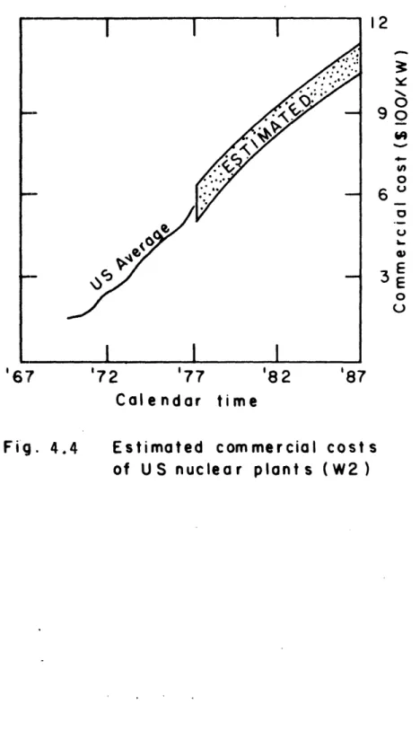
Another study (W2) also has comparable results (see Figure 4.4). It starts with about $153/kWe for all U.S. plants completed in 1970, to $240/kWe in 1972, $518/kWe in 1977, $839/kWe in 1982 and ends with an estimate of $1050/kWe in 1987. Its trend has an average annual increase of $54.5/kWe, which is about 10.5% of the 1977 value. Note also the uncertainty of estimates beyond 1977 in Figure 4.4, which is represented by the shaded band whose half-width is about $64/kWe. In terms of 1977 commercial cost value ($518/kWe), this uncertainty is about 12.4% of the total value. This uncertainty is less than that of Table 2.1. Again regional differences are responsible for the low value reported here

($518/kWe) for 1977 relative to that of the base case.

The MIT's Center for Policy Alternatives conducted a study on LWR capital cost in 1974 (B1). Its early date and, thus, its limited input base, made its findings less dependable. The main contribution of this study is the statistical technique later exploited in a Rand Study (as it will be referred to in this report), which considers capital cost

analysis of LWR plants (M1). The Rand Study is more up-to-date, in the sense it used the widest possible data base available in the winter of 1978. The most interesting finding of the Rand Study is that capital cost is increasing by $140/kWe/year for LWR plants whose Construction Permits were issued in the early 1970s. Figure 4.1 shows that, for the

'72 '77 '82

Cal e nd ar time

Fig. 4.4

Estimated commercial cost

s

of US nuclear plants (W2)

'67

1976-90 period, commercial operation date lags the CP date by about 8 years. By considering the Rand Study projections for commercial cost

versus the CP date, the following results are obtained: Year of Comm. Op. Comm. Cost, $/kWe

1983 1335

1988 2019

1993 2718

1998 3417

This 1988 commercial cost value is 50% higher than that of the base case. The Rand Study concludes that these figures "might well be

realized." Based on our previously discussed findings, we assume in this report that the Rand projections are overestimates and unlikely to be realized.

A possible flaw in the Rand Study may be in the statistical

technique that was developed in the 1974 MIT study, whose shortcomings were pointed out later by Lotze and Riordan (L1). The Lotze/Riordan study shows that LWR and coal-fired plants exhibit similar capital cost behavior. If this is true, along with the Rand Study projections, then by the 1990s both coal and LWRs exhibit economies similar to those of the not-yet-developed technologies.

The main conclusion that can be drawn here is that, based on Figures 4.3.and 4.4, the commercial cost increases linearly at about $55.5/kWe, at a rate about 10% of the 1977 value. This linear increase has resulted in a higher rate of change in the past and will result in a lower rate of change in the future. It is consistent with the 25.8% annual increase for the 1972-77 period.

Thus far our attention has been concentrated on the commercial cost, which may have the alternative definition of being the total capital cost at the date of starting commercial operation. This definition makes the value for commercial cost constant for a given plant. The capital cost, however, is not constant for the same plant. In other words, although commercial cost changes with time if several plants are considered, capital cost changes with time even if one plant is considered. Since the commercial cost value cannot be decreased once the plant is

completed, it thus stands as the minimum value for the capital cost of that plant. After the plant comes on line backfitting expenses are

accumulated on top of commercial cost and thus capital cost of individual plants rises. Such capital cost increase is added to the rate base, and therefore is annually reported to the Federal Power Commission. A study* that concentrated on 10 single-unit plants for the 1971-76 period

investigated this increase (Al). It found that the average accumulated capital cost in 1976 was $155 million per plant. The average annual

increase per plant is $2.40 million for 1971-76 period. This increase is about 1.5% of the 1976 average value. It should be noted here that the $155 million is on a per-plant basis. The average unit capacity in this sample is 595 MWe. This makes the average cumulative capital cost in 1976 to be $250/kWe. This is less than half the 1977 commercial cost value. The reason for this too-low value is that it represents

commercial costs of plants completed between 1968 and 1972, whose annual

*It will be referred to as the S&W (for Stone & Webster Engineering Corp.) Study,, in Chapter III.