Dynamic sonar perception

Dynamic Sonar Perception

by

Richard J. Rikoski

S.M., Ocean Engineering

Massachusetts Institute of Technology, 2001

B.S., Mechanical Engineering and Economics

Carnegie Mellon University, 1998

Submitted to the Department of Ocean Engineering

in partial fulfillment of the requirements for the degree of

Doctor of Philosophy in Marine Robotics

at the

MASSACHUSETTS INSTITUTE OF TECHNOLOGY

June 2003

Massachusetts Institute of Technology 2003. All rights reserved.

Author ...

Department of

O

"'n Engineering

June 1, 2003

Certified by...

John J. Leonard

Associate Professor of Ocean Engineering

Accepted by...

...

Professor Michael S. Triantafyllou Professor of Ocean Engineering Chairman, Departmental Committee on Graduate Students

MASSACHUSETS _INSTITUTE OF TECHNOLOGY

AUG

2 5 2003

Dynamic Sonar Perception

by

Richard J. Rikoski

Submitted to the Department of Ocean Engineering on June 1, 2003, in partial fulfillment of the

requirements for the degree of Doctor of Philosophy in Marine Robotics

Abstract

Reliable sonar perception is a prerequisite of marine robot feature-based navigation. The robot must be able to track, model, map, and recognize aspects of the underwater landscape without a priori knowledge. This thesis explores the tracking and mapping problems from the standpoint of observability. The first part of the thesis addresses observability in mapping and navigation. Features are often only partially observable from a single vantage point; consequently, they must be mapped from multiple vantage points. Measurement/feature correspondences may only be observable after a lag, and feature updates must occur after a delay. A framework is developed to incorporate temporally separated measurements such that the relevant quantities are observable. The second part of the thesis addresses observability in tracking. Although there may be insufficient information from a single measurement to estimate the state of a target, there may be enough information to observe correspondences. The minimum information necessary for a dynamic observer to track locally curved targets is derived, and the computational complexity is determined as a function of sonar design, robot dynamics, and sonar configuration. Experimental results demonstrating concurrent mapping and localization (CML) using this approach to early sonar perception are presented, including results from an ocean autonomous underwater vehicle (AUV)

using a synthetic aperture sonar at the GOATS 2002 experiment in Italy. Thesis Supervisor: John J. Leonard

Acknowledgments

In appreciation of their efforts over my graduate career, I would like to suggest that the non-dimensional numbers in my thesis be named as follows:

N, = the Leonard number

N3 = the Henrik number (Schmidt was already taken) N4 = the Kuc number

N5 = the Choset number

N6 = the Xanthos number

N7 = the Kimball number

N8 = the Damus number

N2 will be left to the reader to name.

Of course, none of this would be possible without the other members of the marine

robotics laboratory, including Jacob Feder, Tom Fulton, Chris Cassidy, Sheri Chang, John Fenwick, Mike Slavik, Jay Dryer, and Paul Newman. And of course, thanks to my family.

This research has been funded in part by NSF Career Award BES-9733040, the MIT Sea Grant College Program under grant NA86RG0074, and the Office of Naval Re-search under grants N00014-97-0202 and N00014-02-C-0210.

Contents

1 Introduction

1.1 Why Marine Robots?

1.2 Enabling Technologies

1.3 Thesis Goals . . . . 1.4 Thesis Outline . . . . .

2 Problem Formulation

2.1 Representations for Navigation 2.2 Stochastic Mapping . . . . 2.2.1 State Projection . . . . . 2.2.2 Feature Mapping . . . . 2.2.3 Measurement Update . . 2.3 Research Issues ... 2.4 Perception . . . . 2.4.1 Analyzing the Perception 2.4.2 Visual Perception . . . .

2.5 Sonar Perception . . . . 2.6 Non-accidental Features . . . .

2.7 Summary . . . . 3 Stochastic Mapping with Working

3.1 M otivation . . . . 3.2 Problem statement . . . . Problem 20 20 25 27 33 34 34 38 40 41 42 44 45 48 50 54 59 62 64 64 65 Memory . . . . . . . . . . . . . . . .

3.2.1 General formulation of the problem . . . .

3.2.2 Linear-Gaussian Approximate Algorithms for CML . .

3.2.3 Data Association . . . .

3.3 Solution to Stochastic Mapping Shortcomings . . . . 3.4 Stochastic Mapping with Working Memory . . . . 3.4.1 Delayed Decision Making . . . . 3.4.2 Batch Updates . . . . 3.4.3 Delayed Initializations . . . . 3.4.4 Mapping from Multiple Vantage Points . . . . 3.4.5 Using Partially Observable Measurements (Long Baselir igation ) . . . . 3.4.6 Mosaicking and Relative Measurements . . . . 3.4.7 Spatiotemporal Mahalanobis Testing . . . .

3.5 Cooperative Stochastic Mapping with Working Memory . . . . 3.5.1 Cooperation with Perfect Communication . . . . 3.5.2 Cooperation with Delayed Communication . . . .

3.5.3 Cooperation with Communication Dropouts or Robots portunity . . . . 3.5.4 Cooperative Mapping of Partially Observable Features

3.5.5 Cooperative Spatiotemporal Mahalanobis Testing . . . 3.5.6 Perception . . . .

3.5.7 Composite Initialization . . . .

3.6 Examples Using Manual Association . . . .

3.7 Integrated Concurrent Mapping and Localization Results . . . 3.8 Related Research . . . . 3.9 C onclusion . . . . 65 68 . . . . 69 . . . . 71 . . . . 71 . . . . 76 . . . . 77 . . . . 78 . . . . 78 ne Nav-. Nav-. Nav-. Nav-. 80 . . . . 80 . . . . 82 82 83 83 of Op-84 86 87 87 89 89 103 111 .112

4 Trajectory Sonar Perception

4.1 Introduction . . . . 4.2 A Simple Feature Constraint . . . .

113 113 115

4.3 Trajectory Perception . . . . 4.3.1 2D Trajectory Perception . . . .

4.3.2 2D Trajectory Constraint . . . .

4.3.3 3D Trajectory Perception . . . .

4.3.4 3D First Substantial Derivative Range . . .

4.3.5 3D First Substantial Derivative in Azimuth

4.3.6 3D First Substantial Derivative of Elevation

4.3.7 Second Substantial Derivative of Range . . . 4.3.8 3D Trajectory Constraint . . . .

4.4 Bat Tones . . . . 4.5 Non-dimensional Analysis . . . . 4.6 Effects of Ocean Waves . . . . 4.7 Complexity Analysis . . . . 4.8 Experimental Results . . . . 4.9 Conclusion . . . . . . . . 118 . . . . 119 . . . . 123 . . . . 124 . . . . 125 . . . . 126 . . . . 127 . . . . 128 . . . . 130 . . . . 131 . . . . 132 . . . . 136 . . . . 138 . . . . 141 . . . . 143

5 Results From an Ocean Experiment 148 5.1 Experiment description . . . . 148

5.2 Selection of the Trajectory Sonar Equations . . . . 149

5.3 Experimental Results . . . . 149

6 Conclusion 167 6.1 Sum m ary . . . . 167

6.2 Conclusions . . . . 168

6.3 Recommendations for future work . . . . 169

A Initialization Functions 172 A.1 Functions for Initialization of Features from Multiple Vantage Points 172 A.1.1 Initializing a Point from Two Range Measurements . . . . 172

A. 1.3 Initializing a Line from a Range Measurement and a Colinear

P oint . . . 178 A.1.4 Initializing a Point from a Line and a Range Measurement . . 180 A.1.5 Initializing a sphere from four spheres . . . . 180

List of Figures

1-1 The REMUS AUV... 21

1-2 The Odyssey Ilb and Odyssey III AUVs . . . . 22

1-3 The Autonomous Benthic Explorer. . . . . 23

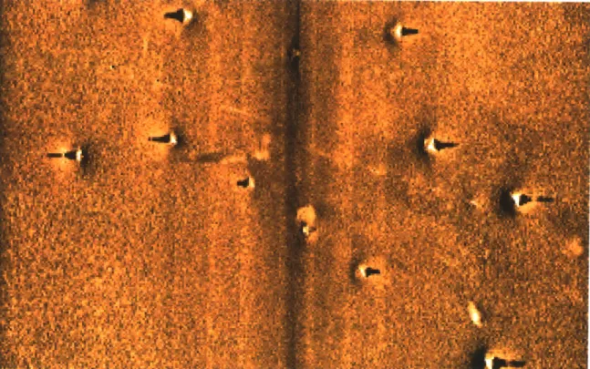
1-4 The generic oceanographic array technology sonar (GOATS) concept. 28 1-5 A sidescan image of targets observed during GOATS 2002. . . . . 30

1-6 Imagenex sonar data... .. ... .... . . 31

1-7 A bat chasing a moth (from [4]).. . . . . 32

2-1 Hand-measured model of a corridor (total length approximately 25 m eters). . . . . 47

2-2 Raw laser and sonar data. . . . . 47

2-3 The Kanizsa triangle. . . . . 60

2-4 A white square. . . . . 60

2-5 A neon blue square... .. ... . ... 61

2-6 A comparison of sonar data representations. . . . . 62

3-1 Comparison of stochastic mapping with and without working memory. 88 3-2 Dead-reckoned trajectory of robot 1. . . . . 93

3-3 Correlation coefficients between elements of a trajectory. . . . . 94

3-4 Initializing partially observable features. . . . . 94

3-5 M ap after initializations. . . . . 95

3-6 Map after a batch update. ... ... 95

3-7 Mapping a second robot. . . . . 96

3-9 3-10 3-11 3-12 3-13 3-14 3-15 3-16

3-17 Raw sonar data for experiment with two point objects. 3-18 Estimated error bounds for the experiment.

Raw data for corridor experiment, referenced Estimated trajectory in a corridor. . . . . .

. . . . 106

to odometry. . . . . 107

. . . . 108

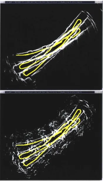
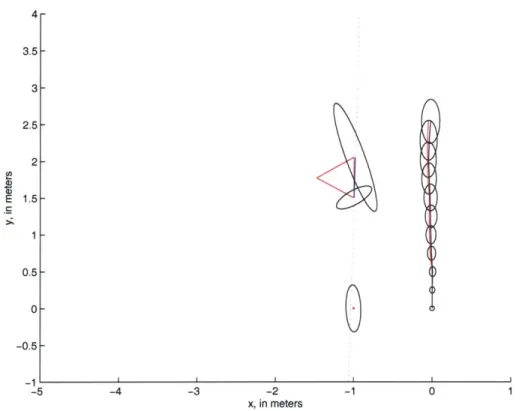
Illustration of naive correspondence . . . . Cartesian projection of measurements. . . . . Raw projection of measurements. . . . . Measurements trajectories for experiment 1. . . . Map from experiment 1. . . . . Cartesian projection of measurements. . . . . Raw projection of measurements. . . . . Measurements trajectories for experiment 2. . . . Map for experiment 2. . . . . 140 143 144 144 145 145 145 146 146 Odyssey III AUV with SAS sensor. . . . Raw sonar data. . . . . Sonar triggers. . . . . Trajectories used for navigation. . . . . . Trajectories used for navigation. . . . . . Trajectories used for navigation . . . . . Measurements from trajectories in global Initializing feature 89. . . . . . . . . 151 . . . . 152 . . . . 153 . . . . 154 . . . . 155 . . . . 156 coordinates. . . . . 157 . . . . 158

Estimating the trajectory of a second robot. . . . . Final map using a second robot. . . . . Uncertainty in the x coordinate of a cooperating robot. . . . . . B21 mobile robot in the plywood box. . . . . Measurements made from 50 positions. . . . . Measurements used to initialize a nine degree of freedom object. Map after initializations. . . . . Measurements used to update the individual feature primitives. . . 98 . . 99 . . 99 . . 100 . . 101 . . 102 . . 103 . . 104 105 3-19 3-20 4-1 4-2 4-3 4-4 4-5 4-6 4-7 4-8 4-9 5-1 5-2 5-3 5-4 5-5 5-6 5-7 5-8

5-9 5-10 5-11 5-12 5-13 5-14 5-15 5-16 5-17 A-1 A-2 A-3 A-4 Measurement trajectory 89. . . . . Global projection of trajectory 89. . . . . Initializing feature 119. . . . . Initializing feature 89. . . . .

Initializing feature 89. . . . .

Final m ap. . . . . CML and GOATS trajectory . . . . T argets . . . .

A sidescan image of targets observed during GOATS 2002.

Two range observations of the point (x,y). . . . .

Two lines tangent to two circles. . . . . Two range observations of the point (x,y). . . . .

Two range observations of the point (x,y). . . . .

159 160 161 162 163 164 165 166 166 173 176 176 178

List of Tables

3.1 Details for the ten manually-selected returns used for feature initial-ization . . . . 93 3.2 Method of initialization for features. . . . . 94

3.3 Comparison of hand-measured and estimated feature locations for points features (in m eters). . . . . 96

3.4 Details for the nine manually-selected returns used for feature initial-ization . . . . 102

3.5 Method of initialization for the feature primitives and comparison of hand-measured and actual locations for the four corners of the box. . 102

Nomenclature

A = feature covariance at initialization B = _{feature/map covariance at initialization}

c = _{speed of sound, approximately 1500 7 in water}

D = spacing between elements for a binaural sonar

f = frequency, of sound

f,

f(.) = vehicle dynamic model

FX = vehicle dynamic model Jacobian

g = gravitation acceleration, 9.8 2

g(.) = feature initialization model

GX= feature initialization Jacobian h = water depth

h(.) = measurement model Hx = measurement Jacobian

k = time index

k = wave number (acoustic wave)

K = wave number (ocean wave)

L = array length

m = measurement degrees of freedom

n = feature degrees of freedom

N, = non-dimensional number describing contribution of velocity to range rate

N2 = contribution of velocity to range second derivative

N3 = contribution of yaw rate to range second derivative

N4 = contribution of acceleration to range second derivative

N5 = contribution of robot velocity to target bearing rate

N7 = contribution of deep water waves to range rate N8 = contribution of shallow water waves to range rate

p = roll rate

pa = apparent roll rate P = state covariance

Pff = covariance of all features Prf = robot/feature covariance Prr = covariance for all robot states

Priri = covariance for all of robot l's states

Priri (k k) = robot l's covariance at time k given information through time k

q = pitch rate

q,,= apparent pitch rate

Q

r = yaw rate

ra = apparent yaw rate

rm = measured range to a target

rc= range to the center of curvature of a target R = measurement noise covariance

T = TOF, measured by the left transducer of a binaural sonar

Tr = TOF, measured by the right transducer of a binaural sonar TOF time of flight

u = surge, or forward velocity Ua = apparent surge velocity v = sway, or side velocity

Va = apparent sway velocity

Va = apparent velocities

Va = apparent accelerations

V = vehicle speed V = vehicle acceleration w = heave, or vertical velocity

Wa = apparent heave velocity x = globally referenced x position

x = globally referenced x velocity x = globally referenced x acceleration

x= x component of center of curvature of target in body coordinates

xc= center of curvature of target in body coordinates

Sc= velocity of center of curvature of target in body coordinates

c= acceleration of center of curvature of target in body coordinates

x = true state

x[k] = true state at time k

x = estimated state

k[klk] = estimated state at time k given information through time k

x[k + 1k] = estimate at time k + 1 given information through time k (prediction) R[k - 1 k] = estimate at time k - 1 given information through time k (smoothing)

Xr = robot's state

xr = set of robot states

Xr1 = for multiple robots, robot l's trajectory

xri(k) = robot l's state at time k

xf = set of all feature states

xf₁ = feature l's trajectory, for a dynamic feature

x₁₁ (k) = feature l's state at time k y = globally referenced y position

y

Yc = y component of center of curvature of target in body coordinates z, = z component of center of curvature of target in body coordinates

Zk = set of all measurements made through time k z[k] = set of measurements made at time k

Za[kl = measurements from time k which have been associated with features Z-,a[k] = measurements from time k which have not been associated with features

Zf [k] = measurement at time k of feature i

z- [k] = measurement of feature m by robot n and time k

A = wavelength (acoustic wave) A = wavelength (ocean wave) r/ = ocean wave elevation

v = innovation

0 = vertical angle of target p = radius of curvature

= variance of x

-xy = covariance of x and y

Ob= sonar beam half angle

0 = target bearing

Or = vehicle heading

r= robot yaw rate, two dimensional wa = apparent angular rate of robot

W = angular frequency (acoustic wave)

Q = angular frequency (ocean wave)

Chapter 1

Introduction

It looks like a torpedo, but this device doesn't explode. It searches for mines and other objects that do. The Woods Hole scientists who built it over the course of ten years dubbed their handiwork REMUS, for Re-mote Environmental Monitoring UnitS. In their first-ever use in hostile waters, the undersea drones were used as part of a team that helped to clear mines from the Iraqi port of Umm Qasr, according to the US Office of Naval Research. Their success allowed 232 tons of badly needed food, water, blankets, and other supplies to reach Iraqi civilians over the week-end. ... Before REMUS is put to work, two sound-emitting transponders are placed in nearby waters and their positions set by portable global navigation devices.

"Undersea drones pull duty in Iraq hunting mines", Jack Coleman, Cape Cod Times, 2 April 2003.

1.1

Why Marine Robots?

Few environments justify mobile robots as well as the ocean. Ocean exploration is hazardous and expensive - robots costing hundreds of thousands of dollars can pay for themselves in weeks. This thesis investigates feature-based navigation in which the goal is to enable an autonomous underwater vehicle (AUV) to build a map of an unknown environment while concurrently using this map for navigation. This capability is anticipated to significantly increase the autonomy and reliability of AUV operations for a wide range of ocean applications.

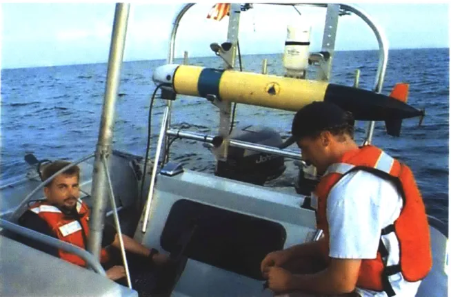
Figure 1-1: The REMUS AUV, developed by the Ocean Systems Laboratory of the Woods Hole Oceanographic Institution (Courtesy of Timothy Prestero).

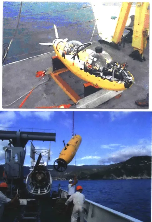
As illustrated by the successful deployment of REMUS in the Second Gulf War, the field of AUV research has advanced dramatically over the last decade. Other successful recent AUVs include the Odyssey class of vehicles (Figure 1-2), developed

by MIT Sea Grant, and the Autonomous Benthic Explorer (ABE), developed at the

Deep Submergence Laboratory of the Woods Hole Oceanographic Institution (Fig-ure 1-3). Ten years ago, these vehicles were being placed in the water for the first time [11, 95, 84]. Today, these AUVs are highly capable and reliable platforms, and many new applications are coming to fruition. Many difficult research issues, however, still remain.

Deep sea exploration is expensive and dangerous. Ocean vessels typically cost

$25,000 per day to operate. Any device that can shorten the time needed to

ac-complish a mission will save money. Ocean exploration is dangerous. Manned sub-mersibles are subjected to environmental extremes unseen in other applications and require expensive life support systems. Underwater construction using compression

Figure 1-2: Top: MIT Odyssey IIb autonomous underwater vehicle with outer, free-flooding hull opened, exposing payload pressure spheres. Bottom: MIT Odyssey III autonomous underwater vehicle shown during the GOATS-2002 experiment (NATO

SACLANT Research Centre).

200-400 L... 600 800 1000 1200 1400 200 400 600 800 1000 1200 1400 1600 1800 2000

diving and exotic gas mixtures is risky. The use of robots potentially allows us to avoid these risks and expenses.

For instance, towed sonar sleds are often used for deep sea surveying [45]. To tow a sled at a depth of several kilometers, a significantly larger amount of cable needs to be used since drag dominates the tension. While the drag of the sled is insignificant, the drag of the cable dominates. A ship dragging a ten kilometer cable can take up to twelve hours to turn around, at a cost of roughly $10,000 per turn. An untethered survey robot can turn around in a fraction of a minute, and many robots can be deployed by a single ship.

Oceanographers are interested in the temperature and salinity of ocean water as a function of depth. Seawater density drives ocean flows. Assuming that the density of seawater will vary inversely with temperature is often inadequate. As it warms, seawater expands, reducing its density. However, at the surface evaporation takes place, increasing the salinity and density. These two conflicting mechanisms make ocean flows unstable [97]. To estimate ocean flows, oceanographers gather conductivity, temperature, and depth (CTD) data. (The salinity is determined by the conductivity.) A typical ocean survey uses a system of cannisters lowered on a cable. At each relevant depth, a cannister opens and gathers water. This sort of survey typically takes four hours.

The Flying Fish [16] AUV was developed to expedite such surveys. A streamlined vehicle without a propeller, the Flying Fish is driven entirely by buoyancy. Initially it has a chunk of lead in the nose and dives at 9, sampling water on the way down. Once the vehicle reaches its bottom depth, the lead is released, and it surfaces at 91. Using a unique recovering mechanism (it is snagged by a second robot), this AUV's entire mission can be completed in forty minutes.

Manned exploration of the deep sea is expensive in part due to the necessity of life support systems. First, the pressure makes the environment extremely challenging. In space, the difference between the inside and outside pressure is one atmosphere, or roughly 100kPa. Moreover, the pressure vessels are typically in tension. Underwater, a "full ocean depth" vehicle has to withstand a compressive load of 600 atmospheres,

or roughly 60MPa. By convention, 6000m is considered full ocean depth, and a vehicle designed for 6000m will be able to access the vast majority of the ocean. However, when the Trieste bottomed out in the Marianas trench, it was closer to 11, 000m, or a pressure of lIOMPa. Since these are compressive loads, pressures that a vessel might withstand in tension can cause a buckling failure. To avoid buckling, spherical pressure vessels are often used. The manned submersible Alvin has a 2m diameter, four inch thick titanium sphere which has a limited fatigue life.

Near hydrothermal vents, water temperatures are high enough that, in the absence of light, the rocks glow red hot. The water exiting the vents is hot enough to melt the windows of Alvin.

A submersible can become entangled in seaweed, trapped under an overhang,

disabled due to a battery failure, or lose its life support systems. Once, Alvin came under attack from a swordfish. The safety record of manned ocean exploration is a testament to the engineers who design and maintain the craft. However, this comes at a price, and clearly there is a strong rationale for unmanned exploration with robots Even at a cost of hundreds of thousands of dollars, a robot that can save the user $10, 000 every time it turns around can be economically justified. A robot that saves thousands of dollars per CTD survey and dive multiple times per day can be economically justified. A robot which spares the user the costs associated with saving or losing human lives can also be justified. A tremendous amount of money is spent on ocean exploration, and what would seem an outrageous sum for a land robot is a sound investment in the marine community.

1.2

Enabling Technologies

There are a multitude of problems that must be solved for marine robots to become pervasive. Five key marine robotics research areas are power, locomotion, navigation, perception, and cognition.

Power consumption and energy source design are critical to any deployment. Robots should be designed to minimize the hotel load (the non-propulsive power

draw) and travel at a velocity that optimizes range [15]. Batteries or alternative en-ergy sources such as fuel cells need to be developed to provide the greatest neutrally buoyant energy density [79, 1].

Locomotion is another serious design issue. The dynamics of a robot depend substantially on the design goals. An AUV such as REMUS [89] that is designed to perform sidescan sonar surveys could have a simple, streamlined design. An ROV like JASON [7] that manipulates objects, such as amphora, might be better designed as a hovering vehicle.

Navigation is a chronic underwater problem. GPS is unavailable because wa-ter quickly attenuates electromagnetic signals. Inertial navigation systems drift over time. Dead reckoning leads to unbounded error. The best solution is to use a cali-brated network of underwater beacons. This is how REMUS and most other AUVs navigate today. The use of beacons increases the cost and reduces the flexibility of marine robot deployments. The ultimate goal for our research is for robots to navigate relative to distinct aspects of terrain.

Navigating relative to terrain will require substantial advances in the fourth key marine robotics research area: perception. Perception is the process of transforming sensory data into higher level representations, or constructs. Simple examples of perception include triggering on signals that exceed thresholds and rejecting spurious measurements. High-level perception typically concerns object recognition and may involve comparing high-level representations to other high-level representations. This thesis will examine methods for processing sensory data towards the ultimate goal of terrain based navigation.

Cognition is the final, and perhaps least explored, marine robotics problem. Given that a robot has the perceptive capacity to develop an understanding of its surround-ings, it would be desirable for the robot to autonomously achieve some broader goal. Most marine robots are either directly controlled by people (such as ROVs) or are preprogrammed to follow specific paths (survey vehicles such as the Odysseys, Ocean Explorer, ABE, and REMUS). With the development of cognition, it will become feasible to consider a richer variety of robot-feature interactions. We could consider

having robots perform minor tasks such as picking things up or repairing or building simple structures.

The generic oceanographic array technology sonar (GOATS) concept, illustrated in Figure 1-4 [83], provides a compelling vision for AUV technology development. The overall goal is to enable networks of many AUVs to rapidly survey large areas and to detect and classify objects in real time.

1.3

Thesis Goals

This thesis concerns feature-based navigation. At the most primitive level, the feature-based navigation problem can be broken down into: 1) finding features, 2) building a map of features, and 3) recognizing features. Finding and recognizing fea-tures using sonar has received little attention in the robotics literature compared to the equivalent problem in vision. The first part of the thesis develops a framework for mapping partially observable features. The second part of the thesis develops meth-ods for early tracking of features. Object recognition is left for future work. For the purposes of this thesis, grouping measurements based only on measurements, without knowing what the target is, over extremely short time scales, will be considered early tracking or correspondence. Recognizing targets after prolonged periods without ob-servations will be considered object recognition and will be left as future work. This thesis will be restricted to very short time scales on the order of ten seconds.

We want robots to navigate. We want to send them places, have them get there, and have them return successfully. We would like them to explore environments, find noteworthy things, come back, and either tell us how to get to those things or return to them themselves. On smaller scales, we would like for robots to develop an understanding of an environment so they can maneuver around obstacles, manipulate objects, and perform other high-level robot/object tasks.

Some robots possess some of these capabilities. Using GPS or inertial navigation, robots have been able to visit predefined areas. Using homing beacons or predefined targets, some robots have returned to areas and docked. Obstacle avoidance

tech-4

vsw

+74

~@

Figure 1-4: The generic oceanographic array technology sonar (GOATS) concept. The vision of GOATS is to enable a network of multiple AUVs to perform rapid detection and classification of proud and buried targets over large areas using multi-static acoustic sensing.

Bh

+

niques have been developed for collision avoidance. Industrial robots have performed manipulation tasks in highly controlled environments, but what we want goes further. We want robots to enter environments and use their sensors to develop true situa-tional awareness. We want them to do this without external beacons or homunculi. We want feature-based navigation.

The goal of feature based navigation just leads to more questions. What does it mean for a robot to be situationally aware? How should it use its sensors to develop an understanding of its environment? How does this depend on the environment? Are these goals achievable?

For the purposes of this thesis, we will restrict situational awareness to simply understanding environmental geometry. In other words, the robot has to understand where things are well enough to get around. This is still very open ended, as no specific environmental representation has yet been chosen.

The perception problem, or how the robot should use its sensors to build an understanding of the world, is arguably the toughest problem in robotics. The world is ambiguous, partially observable, cluttered, complicated, and dynamic. What is required of perception, and hence the form of the instantiation, depends significantly on the selected world representation.

Conventional undersea sonar data interpretation is based primarily on an imaging paradigm. The goal is to utilize as narrow beams as possible to attempt to create sharp pictures that a human operator can readily interpret. For example, Figure 1-5 shows a 500 kHz sidescan sonar image for a set of undersea targets observed during the GOATS 2002 experiment. Figure 1-6 shows data from a 675 kHz Imagenex mechanically scanned sonar taken in a tank. Each of these sensors has a beamwidth on the order of 1 degree. While these images display some acoustic artifacts, such as multipath in the tank sonar image, a well-trained human operator can clearly make some inferences about the structure of the scene being imaged.

Part of the rationale for the design of imaging sonars is to get as few pings as pos-sible on a given target. Then, using many pings obtained systematically over a given area, one can create a picture. However, if we look at the design of biosonar systems,

Figure 1-5: A sidescan image of targets observed during GOATS 2002 using a Klein

DS5000 500 kHz sonar system. The narrow beams of the Klein sonar provide images

in which the shadows cast by objects are clearly visible. (Image courtesy of GESMA.)

A (a)

(b)

Figure 1-6: (a) Imagenex 675 kHz mechanically scanned sonar. (b) Sonar data ac-quired with this sensor in a testing tank. The tank is roughly three by three meters in dimensions with four cylindrical posts protruding upwards at several locations in the tank.

Figure 1-7: A bat chasing a moth (from [4]).

we see a divergence from the way that man-made sonar systems are developed.

A motivation for the approach that we follow in this thesis comes from the

remark-able sonar capabilities of dolphins and bats [4, 2]. In contrast to man-made imaging sonars, bats and dolphins employ wide beams. They also utilize dynamic motion strategies when investigating and tracking targets. For example, Figure 1-7 shows a bat attempting to capture a moth. The motion of the bat clearly differs from the way in which a man-made sonar sensor is typically scanned through the environment. The question of how to exploit dynamic motion control for echolocation with a wide beam sonar has not received much attention in the the undersea robotics community. This is one of the key questions that we consider in this thesis. Can we use a wide beamwidth to advantage? Is it possible to maintain contact with features so that we can continually use them as navigational references?

1.4

Thesis Outline

This thesis has two parts. The first develops a framework for mapping and navigation, creating an explicit infrastructure for delayed perception and mapping of partially ob-servable features. The second part investigates how to perform early sonar perception.

By early sonar perception, we mean the initial tracking of features, prior to modeling

and object recognition.

Chapter 2 reviews prior work in mobile robot navigation and mobile robot sonar usage. Chapter 3 develops stochastic mapping with working memory, a new frame-work for mapping and navigation in situations with partial observability. Chapter 4 develops an early correspondence technique based on the minimal information nec-essary to track locally curved objects. Chapter 5 presents results from the GOATS 2002 AUV experiment. Finally, Chapter 6 provides a summary of our contributions and makes suggestions for future research.

Chapter 2

Problem Formulation

This chapter formulates our approach to the problem of feature-based navigation using wide beam sonar. We begin by discussing the task of choosing a representation for navigation and mapping. We proceed to review the feature-based formulation of the concurrent mapping and localization (CML) problem, the approach that we follow due originally to Smith, Self, and Cheesemman [87]. After discussing some of the open issues in CML research, we proceed to formulate our approach to the sonar perception problem. We discuss relevant work in computer vision, such as optical

flow, that inform our investigation of widebeam sonar perception for feature-based

navigation. The principle of natural modes [81] serves as a guiding principle for developing percerptual models.

2.1

Representations for Navigation

It is necessary to identify and define the parameters of successful robot navigation. For instance, suppose we want to send a robot to an arbitrary location. How should it proceed, and how will it know that is has gotten there?

If the distance to be travelled is short, the robot could use dead reckoning [12]. By

estimating its heading and velocity, the robot can estimate its position, maneuvering until it believes it is at the final location. Typically, when dead reckoning, the robot uses a model of its dynamics, its control inputs, and measurements such as heading

a compass or gyro and velocity from a Doppler Velocity Log (DVL). Unfortunately, when the robot dead reckons, errors grow with distance travelled and time. An inertial navigation unit could be used to reduce the error growth rate [56], but inertial navigation also results in unbounded error growth.

For long transits, in which dead reckoning and inertial navigation are insufficient, the robot will need to use external information. We need to define what external information is required, and how the robot should use that information. This leads directly to the heart of the feature-based navigation problem; the choice of a represen-tation. There are two major forms of feature based navigation: procedural navigation

and globally referenced navigation.

If procedural navigation is used, the robot transits from place to place without knowing where it is globally (ie having its position defined in a coordinate system). Instead, it uses an ordered set of instructions. Navigation is decomposed into behav-iors and cues. For instance, the following are directions, taken from an (uncorrected) e-mail for how to get to an MIT laboratory.

NW13-220 You can get in either by showing your ID at the front door of

the reactor and heading up the stairs then down the hall make a right, through the doors and my lab is right there, my office is inside or by going in NW14 up the stairs down the hall a bit first left through the red doors, all the way down the hall through another red door, then another, right down the hall first left and my office is right before you get to the grey doors.

Such instructions presuppose high-level object recognition such that one can rec-ognize "the red doors" in order to turn left through them.

The advantage of this approach is that by decomposing navigation into paths and cues, if one can recognize the cues and stay on the paths, then navigation is fairly assured. Similar approaches have been used nautically. River navigators cannot stray from their path, ignoring obstacle avoidance issues (trees and sandbars can be par-ticularly hazardous) a navigator only needs to recognize when they approach the appropriate city [26]. Navigation along coastlines proceeds similarly. Polynesian nav-igators [64] travelled between islands using "star paths". By steering at the location

where a sequence of stars appeared on the horizon, they could maintain a constant heading and steer towards a distant island. For landfall, birds were observed at dawn and dusk. At dawn, birds would fly out from shore to feed, at dusk they would fly home. The heading of the birds defined a path to the island.

Consider a second example:

Hugh Durrant-Whyte: Where's the bathroom?

John Leonard: It's left, then another left, and on your left. Do you

want Rick to show you?

Hugh Durrant-Whyte: That's ok, I'll find it, it's left, left, and then

left?

(10 minutes pass)

Hugh Durrant-Whyte: Now how do I get to the airport?

Clearly, Durrant-Whyte's trip to the bathroom takes advantage of substantial prior knowledge, but it is a very procedural trip. Leonard does not provide a globally referenced bathroom position; rather he provides a set of instructions. Given sufficient perceptive and cognitive capabilities, including some prior knowledge of hallways and bathrooms, one can parse the instructions and arrive at the desired destination. One might wonder about the phrasing of the questions. In the first, he asks "where", in the second, he asks "how". Perhaps for things that are very close, a vectorized approach is occasionally sufficient, but for distant objects, a procedural representation is necessary. Or perhaps we have over analyzed his diction.

Examples of procedural navigation in robotics include the behavior based navi-gation of Mataric and Brooks [18], the cognitive mapping of Endo and Arkin [31], the semantic spatial hierarchy of Kuipers [55], and the usage of generalized Voronoi graphs by Choset [24] .

Mataric and Brooks [18] developed a robot that navigated based on its reactions to the environment. The robot had behaviors such as obstacle avoidance and wall following. By establishing sequences of behaviors that resulted in the robot being in specific locations, a sort of robotic portolan [26] was established.

Similarly, Endo and Arkin [31] created a cognitive map, which includes both spatial and behavioral information. The goal was to create a representation that

adequately represented the information needed to move between locations.

Choset [24] used a Generalized Voronoi Graph (GVG) for navigation. The GVG is essentially a set of points that are equidistant from the closest objects. In the planar case, a sort of lattice with curves is generated. The nodes of the GVG are of special importance, for they define locations where numerous objects are equidistant. Once a GVG is defined, localization can occur simply by knowing which nodes the robot is between.

Globally referenced navigation differs from procedural navigation by representing the robot position in terms of globally referenced coordinates. Such coordinates could be latitude and longitude or a locally referenced coordinate system. The robot maps terrain, and by reobserving terrain estimates its globally referenced position. Some of the key questions include how terrain should be modeled, how the terrain should be mapped, and when terrain is reobserved, how that information should be used to improve the robot's estimate of it's locatoin?

Hybrid metric/topological representations, consisting of a network of places or submaps, have been successfully exploited for mobile robot navigation and mapping

by a variety of researchers including Kuipers [55, 54], Gutmann and Konolige [40],

and Thrun [91, 94].

Arguably, one of the most successful feature based navigation approaches is the globally referenced grid based approach of Thrun [91]. Using a combination of oc-cupancy grids and particle filters, Thrun estimates the true probability distribution of measurements, which is in turn used for navigation. However, discrete features are not represented, so it is unclear how this scales to higher level operations such as manipulation.

An alternative approach, termed "stochastic mapping" after a seminal article

by Smith, Self, and Cheeseman [87], breaks the world down into discrete modeled

features. By combining reobservations with an extended Kalman filter, measurements of objects are used for navigation. This is the approach that we follow in this thesis. In the next section, we review the stochastic mapping approach and illustrate it with a simple two-dimensional example. In the following section, we discuss some of the

active research topics in the field of CML today, such as the map scaling problem and the data association problem.

2.2

Stochastic Mapping

Stochastic mapping is a feature-based, Kalman filter based approach to mapping and navigation relative to a global reference that was first published by Smith, Self, and Cheeseman [87] and Moutarlier and Chatila [70].

The stochastic map consists of a state vector x and the covariance P. The state vector x[kIk] contains the robot state x,[kIk] and the feature states xf[k k]. We use the variable k to represent discrete timesteps.

x[klk]- Xr[kjk]

1(2.1)

xf [kI k]J

For a two dimensional example, a robot's state could be its x and y coordinates, its heading 6, and its velocity u

Xr[klk] =

Two point features, xf, and xf2, would be

Xf[klk] [

xf2 [k 1

In this case, xf[kIk] is the vector of features vidual feature vectors.

The state vector describing the map wou Xr Yr

(2.2) Or

described by their respective coordinates

Xf₁

(2.3)

Yf2

indi-Exr[k~k]

1

j

I

The covariance P, which describes the uncertainty in the state vector, would be

p[Prr

Prf

[Pfr Pif

J

For the described two dimensional world, the covariance would be

(2.5) [Prr PrI -Pfr Pff Prr Pfir Pf2r

Decomposing the robot covariance would yield 2

X~r, UXrYr 0*XrOr UXrU %rr 2

Yr Xr ayr Uyr Or (-yr U

Or-r Xr JOr Yr 27 9Uxr (TUYr (7U~r

JOinU 2

ou

Similarly, the decomposed state covariance would be

Prfi Prf2 Pf1f1 Pf1f2 Pf211 Pf 2f2 _. (2.6) (2.7)

2

X 2 U U7rrOxrOr UXU QVxrx 1 X~ 0 UrYf1 XrXf 2 CrvrYf 2

Xr r rYr r O rU orf or a (y

yrzr Y r 0yrU dYrXf 1 YrYf 1 YrXf2 GYrYf2

Orrr

U0ryr U, U (7OrXfl UOr Yf 1 rOrXf2 UOrYf2

r UXr UYr CUOr dU JUXf1 GUYf 1 UUXf₂ Uyf2

Prr = r~ rf1Y 7fO rfU ( .X (2.8)

~Xlr Xl~ j.j~r0f1 ~Xf1 07Xf 1Yf 1 rXf 1Xf 2 rXf IYf 2

f 1Xr rYf1Yr _{fiz Jyiyr69/0,Gyfn} UYf1 Or CfiU _Jfizi Yfi 1 _yfi f 1f %fif2 _Jyfif2 U2fyf2_GYflzf2

(T2

UXf2Xr 1Xf2Yr 1Xf₂0r Xf2 U Xf2Xf1 UXf₂yf X1 zf2 OXf2Xf2

(T a 2

Lf2Xr UYf2Yr %Yf2Or OYf2U %Yf2Xf1 UYf₂Yf₁ OYf2Xf2 yf2 J

2.2.1 State Projection

As the robot moves, its positional uncertainty increases. This is due to the uncertainty in velocity and heading, and process noise. A nonlinear function f(-) is used for state projection. An initial state

x[klk] =

[

[

with u[k]) being the control input. For a two dimensional model with control input u[k] = [60r 6u]T, the robot state projection would be

Xr + Ucos(Or) 6t

Xr[k +1Ik] = f(Xr[klk], u[k]) = Yr +u sin(Or)6t (2.11)

Or + 60r U + Ju

P = FXPF, +

Q

where F,, is the Jacobian of the projection function f(.) and

Q

Fx =[Fxr 0 _I

(2.13)

with the vehicle Jacobian Fxr being

Fxr =I+ 0 0 -usin(Or)6t 0 0 u cos(0) 6t 0 0 0 0 0 0 cos(Or)St sin(0,) 6t 0 0 (2.14)

2.2.2

Feature Mapping

Features are mapped by augmenting the feature vector xf of the state vector x using the nonlinear function g(.). For a map with i features, a new feature i + 1 would be mapped at time k using measurement zf,+1 [k] through the following state

augmenta-tion: x[ kk] = Xr[k k] xf[k k] Xr[k

k]

Applying the two dimensional robot model, and measuring the range and bearing to the target, zfi~l [k] = [r 0]T, the initialization function would be

g (xr[kIk], z,+[k]) = x1i*

EYf+

Next, the covariance matrix is augmented using submatrices A and B

(2.17)

where A and B are

A = GxPGxT + GRGT (2.18)

B = GxP. (2.19)

The state and measurement Jacobians G, and G, in this case would be

0 1 -r sin(Or + 0) 0 ...

0

oJ

Lsin(O, + 0) r COS (Or + 0)

If the range and bearing measurements variance would be the diagonal matrix

or2

R =r

L0 If the range and bearing observations wer

nonzero off diagonal terms.

were uncorrelated, the measurement

co-.

(2.22)

e correlated, this would be reflected by

2.2.3

Measurement Update

When measurements of features are made, the state is updated using an extended Kalman filter (EKF) [47, 9]. First, the measurement is predicted using the nonlinear prediction function h(-). Then, the innovation v is calculated, which is the difference between the actual and predicted measurement:

P B T

P =

B A

GX =

v = z - h(().)

The associated innovation covariance S is calculated using the measurement Ja-cobian H,, the state covariance P, and the measurement covariance R

S = HxPHx T + R. (2.24)

Next, the Kalman gain is calculated

K = PH TS-1 (2.25)

Using the Kalman gain, the updated state and covariance can be calculated

x[k + Ilk + 1] = x[k + 1lk] + Kv (2.26)

P=P-KSK (2.27)

For instance, for a robot in a map with a single point feature

x[k k] = Xr Yr

Or

making a measurement z =

[r

h(x(k + ilk)) =

[

2 _{+ (yf1 - Yr)2}

arctan( _{Xf )-Xr}Yf_Yr _ 0r

and would have a measurement Jacobian

(2.29) (2.23)

0r Or Or or Or Or

O_4X r aY r 0O 9- OuOxf 1 6

Yf1 (2.30)

H

=aor aor 00

_Kxr

yr 0 _5U OXf_{1 ayfJ}

or

EXr-Xfi

HX _Yr-Yfl r . (2.31)

Xf₁ Xr-1 0 Yf1 Yr XrXf(

L r r2 r2 r2

2.3

Research Issues

The Smith, Self, and Cheeseman approach to the CML problem has had a profound impact on the field of mobile robotics. Recent events such as the "SLAM Summer School" [25] document the high level of recent interest and progress in the problem of robot navigation and mapping. Topics of recent research in CML include the problems of map scaling, data association, and operation in dynamic environments.

The map scaling problem has been a key issue in CML research. The ideal so-lution to the map scaling problem would simultaneously satisfy the "Three C's" of consistency, convergence, and computational efficiency. The basic Kalman formula-tion of CML by Smith, Self, and Cheeseman suffers an 0(n2_{) growth in computational}

complexity in which n is the number of environmental features. Some methods can reduce the computation by a constant factor but still incur the 0(n2_{) growth. These}

include postponement (Davison [27] and Knight [50]), the compressed filter (Guivant and Nebot [39]), sequential map joining (Tard6s et al.[90]), and the constrained local submap filter (Williams [101]). Approximation methods that achieve 0(1) growth of complexity include decoupled stochastic maping [61] and sparse extended information filters [94, 93]. Recently, Leonard and Newman have developed a submap approach that achieves asymptotic convergence for repeated traversals of the environment while maintaining consistency and 0(1) growth of complexity [57].

One criticism of the Kalman approach to CML is the assumption that Gaus-sian probability distributions can effectively represent uncertainty and can cope with nonlinearities in models for vehicle dynamics and sensor measurements. Several

ap-proaches have been published for a fully nonlinear approach to CML, including the factored solution to simultaneous localization and mapping (FastSLAM) [68], and the use of a sum of Gaussians models for representation of errors [66].

The Atlas framework of Bosse et al. [13] uses a hybrid metric/topological rep-resentation for CML to achieve real-time CML in large, cyclic environments. The approach combines and extends elements of Chong and Kleeman [22] and Gutmann and Konolige [40].

Another assumption of most recent in CML is that the environment consists of static features. Research that lifts this assumption, to integrate tracking of dynamic objects with mapping, has recently been performed by Wang et al. [96] and Hdhnel et al.[41].

The data association problem concerns determining the correspondence of mea-surements to environmental features. Many SLAM researchers have used nearest-neighbor gating [8] for determing correspondence. Joint Compatibility Branch and Bound (JCBB), an improved method that simultaneoulsy considers associations to multiple features, has been developed by Neira and Tard6s [75].

Nearly all of the work in CML listed above assumes that sensors provide complete observations of environmental features from a single vehicle position. This assump-tion, however, is violated in many important scenarios, notably when sensing with wide beam sonar data. In effect, CML assumes perception has been solved. However, as argued in Chapter 1, we feel that perception is arguably the toughest problem in robotics.

2.4

Perception

Perception is the process of transforming raw sensory data into a useful representation so a robot can interact with its environment. Raw sensory data is the output of a sensor. For a simple acoustic sensor, the output could be a waveform or a time of flight (TOF) for ranging. A camera would output an image, typically a bitmap.

output high-level constructs such as, "my thesis advisor is looking skeptically at this sentence." Perception is what transforms raw data into high-level representations.

Sonar research typically differs from vision research in its goals. Quite often, sonar researchers are trying to create an image that a human can process, rather than a representation for automated processing. (For example, see Figure 1-5 in Chapter

1.) When humans process visual images, they have the benefit of a highly evolved

visual cortex, and substantial prior knowledge and reasoning. It would be desirable to develop sonar processing without having to replicate the human visual apparatus. Most robotic perception work using sonar has concerned either obstacle avoidance or feature detection for navigation. Nearly all commercially available land mobile robots come equipped with a ring of Polaroid sonar sensors. Many researchers who have attempted to use sonar data in land robotics have been disappointed due to a fundamental misunderstanding of the nature of sonar data. The Polaroid sonar is a wide beam time of flight sensor (TOF) that typically triggers on specular echoes and which may trigger on multipath reflections. Multipath is when the sound does not travel directly between the transducer and the target but strikes an intermediate object. When multipath occurs, the range to the target is no longer simply the path length divided by two.

The SICK laser scanner became widely available in robotics in the mid-1990s. Reseachers have been much more successful with laser data. Figure 2-2 shows a comparison of SICK laser and Polaroid sonar data taken in a corridor at MIT. The layout of the corridor is shown in Figure 2-1. Both data sets are smeared by dead reckoning error; however, it is readily evident that the laser data provides a much better match to a visual map of the environment.

A smaller number of researchers (such as Kuc, Kleeman, Wijk, Choset, Brooks,

Leonard, and Durrant-Whyte) have investigated how to use sonar in robotics, de-veloping approaches that take advantage of its strengths while accommodating the weaknesses of specific sonar units.

What form the high-level representation takes depends heavily on the cognitive algorithm. For many feature-based navigation approaches, such as Leonard and

Door Door Door Door Door

DDr DOor Door Door Door Dor

Figure 2-1: Hand-measured model of a corridor (total length approximately 25 me-ters).

Figure 2-2: Laser (top) and sonar (bottom) data taken with a B21 mobile robot in the corridor shown in Figure 2-1, referenced to the dead-reckoning position estimate. The vehicle traveled back and forth three times, following roughly the same path. Each sonar and laser return is shown referenced to odometry. The laser data is slightly smeared due to a latency between the odometry and the laser data.

r-Feder [61, 34, 58], Moutarlier and Chatila [71], Smith, Self, and Cheeseman [87], Tard6s et al.[90], Newman [77, 29], and Wijk and Christensen [98, 100, 99], the

out-put must be geometric observations of individual, modeled features. So perception determines which measurements go with which features (the correspondence prob-lem) and establishes correct models for the features (point, plane, cylinder, sphere, amphora, etc.).

Other approaches require less of perception. For instance, by devising a sufficiently complex estimator, Thrun [92] was able to abstract away all aspects of physical real-ity. Rather than decompose the world into features or objects, the world is modeled as a probability distribution. Measurements simply change the world distribution. Alternatively, Mataric and Brooks [18] bypassed traditional cognition, connecting perception directly to control. Rather than use high-level features, very simple per-ception, such as feature tracking, was used to provide an appropriate input for control behaviors.

2.4.1

Analyzing the Perception Problem

Early perception researchers had to address two problems simultaneously. In addition to solving the problems of their field, they had to define a rigorous methodology for

approaching them.

Marr [67] proposed an "information processing" approach, by which perceivers do "what is possible and proceed from there toward what is desirable." Rather than try to transform raw data into a desired representation in a single step, a sequence of transformations is performed. Each transformation is specifically designed with respect to the others and each transformation is rigorously grounded in physics. The information processing transformations were described at three levels.

The first level, the Computational Theory, describes the inputs, outputs, and transformation of a processing stage. An input should be justified based on what can reasonably be expected of precursor processing stages. Any stage that requires an impossible input will likely fail in practice. Similarly, the output of a processing stage should be justified in terms of the broader goal of the processing. Transforming data