HAL Id: hal-01906001
https://hal.sorbonne-universite.fr/hal-01906001
Submitted on 26 Oct 2018HAL is a multi-disciplinary open access archive for the deposit and dissemination of sci-entific research documents, whether they are pub-lished or not. The documents may come from teaching and research institutions in France or abroad, or from public or private research centers.
L’archive ouverte pluridisciplinaire HAL, est destinée au dépôt et à la diffusion de documents scientifiques de niveau recherche, publiés ou non, émanant des établissements d’enseignement et de recherche français ou étrangers, des laboratoires publics ou privés.
What is the tensile strength of a ceramic to be used in
numerical models for predicting crack initiation?
Dominique Leguillon, Eric Martin, Oldřich Ševeček, Raúl Bermejo
To cite this version:
Dominique Leguillon, Eric Martin, Oldřich Ševeček, Raúl Bermejo. What is the tensile strength of a ceramic to be used in numerical models for predicting crack initiation?. International Journal of Fracture, Springer Verlag, 2018, 212 (1), pp.89-103. �10.1007/s10704-018-0294-7�. �hal-01906001�
What is the tensile strength of a ceramic to be used in numerical models for
predicting crack initiation?
Dominique Leguillon • Eric Martin • Oldrich Sevecek • Raul Bermejo
Dominique Leguillon dominique.leguillon@upmc.fr
Institut Jean Le Rond d'Alembert, Sorbonne Université, Centre National de la Recherche Scientifique, UMR 7190, F-75005, Paris, France.
Eric Martin martin@lcts.u-bordeaux.fr
Laboratoire des Composites Thermo-Structuraux, CNRS UMR 5801, Université de Bordeaux, F-33600, Pessac, France.
Oldrich Sevecek sevecek@fme.vutbr.cz
Institute of Solid Mechanics, Mechatronics and Biomechanics, Faculty of Mechanical Engineering, Brno University of Technology, 616 69 Brno, Czech Republic.
Raul Bermejo raul.bermejo@unileoben.ac.at
Institut fuer Struktur- und Funktionskeramik, Montanuniversitaet Leoben, A-8700 Leoben, Austria.
Department of Materials Science and Engineering, The Pennsylvania State University, University Park, PA-16802, USA.
Corresponding author: dominique.leguillon@upmc.fr
Abstract: Criteria for predicting initiation of cracks in brittle materials like ceramics are based
on two parameters: the material fracture toughness and the tensile strength. Standardized experiments exist to estimate the former. However, the tensile strength is often taken from experiments (mainly uniaxial bending) on specimens with various geometries and surface finish, usually tested under ambient conditions at a given loading rate. The reported strength is commonly the Weibull characteristic strength, which scatters due to the critical defect size distribution on the tested specimen. In this work, we propose a definition of the “inherent” or “intrinsic” tensile strength to be used in numerical models, making a distinction between extrinsic defects due to manufacturing and intrinsic ones relying on the microstructure.
Our approach is based on the Finite Fracture Mechanics theory and the Coupled Criterion applied to small surface flaws and its influence on the measured (extrinsic) strength. Numerical results are compared with experiments on alumina reported in the literature. In addition, a model for the Petch law (strength vs. grain size) in polycrystalline materials is proposed using the Coupled Criterion, which predicts an initial crack length of increasing numbers of grains as the grain size decreases.
1. Introduction
The coupled criterion (CC) (Weissgraeber et al., 2016) and the cohesive zone models (CZMs) (Elices et al., 2002) are the most common methods for predicting the crack nucleation in brittle materials. Recent examples include also the phase field methods (PFMs) (Tanné et al., 2018). They require usually two fracture parameters: the material strength and the material fracture toughness. Note that in CZMs the material toughness is sometimes replaced with the critical
opening, but together with the peak stress, it is strictly equivalent to the data of the two previously mentioned parameters. In PFMs the two parameters are the material toughness and the regularization length, but again, even if the equivalence is not as straightforward as for CZMs, it is strictly equivalent to the data of the two previously mentioned parameters (Tanné et al., 2018).
A number of tests are identified and standardized to measure fracture toughness in brittle materials. In particular, uniaxial flexure of prismatic specimens having a defined starting defect (e.g. notch, indent) is widely used for ceramic materials. The commonly used methods are Single Edge Notch Beam (Damani et al., 1996), Surface Crack in Flexure (ISO 18756, 2008), and Single Edge V-Notched Beam (ISO 23146, 2008). Other alternative methods have been recently developed to measure the toughness of brittle components with various geometries, for instance, the Notched Ball test (Strobl et al., 2017), and the Notched-Ball-on-Three-Balls test (Danzer, 2007; Strobl et al., 2014). The Double Cleavage Drilled Compression test on a drilled specimen can also be mentioned (He et al., 1995). In contrast to toughness measurements, determination of the tensile strength in brittle materials is more challenging, especially in ceramics. In fact, strength measurements commonly refer to the “extrinsic” strength of the ceramic material, which is related to the critical defect causing fracture of the testing specimen. Typical defects are surface flaws (e.g. surface pores, pull-outs, grinding grooves, scratches, contact cracks), and volume flaws (e.g. internal pores, agglomerates, aggregates, second phases) introduced during processing, manufacturing, handling, and/or in service (Bermejo and Danzer, 2014). Besides the size of such flaws, their shape and location within the specimen affect the measured strength. For instance, for commonly loading situations, surface flaws are more severe than volume flaws (Danzer, 2014). In addition, the type of test (i.e. tensile, uniaxial or biaxial bending) is known to give different results. This is related to the so-called “strength size effect”, which is the most prominent consequence of the stochastic character of strength in many brittle materials, as interpreted by Weibull theory (Weibull, 1951). This approach provides the probability of failure of a specimen under a given tensile load: the larger the specimen, the greater the probability of encountering a critical flaw and thus the greater the probability of failure. Furthermore, the testing conditions (i.e. loading rate, relative humidity in the environment) can also influence the strength (and toughness) measurements. The presence of humidity in the environment can trigger the “sub-critical” propagation of existing defects, and thus lower the extrinsic strength of the tested specimen (Freiman, 2013; Bermejo at al., 2013; Krautgasser et al., 2016).
An interesting observation in strength measurements is that when diminishing the size of the critical flaw, the increase in tensile strength reaches an upper limit (Danzer et al., 2007). This is explained by the lower level of small natural or inherent (intrinsic) flaws, whereby the grain size is commonly admitted as a first approximation of the critical intrinsic defect length (i.e. the smallest defect size in the material). This upper limit has been identified in many polycrystalline ceramics, but not in glasses (see Usami et al., 1986), which supports the hypothesis that the strength limit, what we define as the intrinsic strength (Taylor (2007) uses the denomination inherent strength), may be related to the grain size of the material.
The aim of this paper is to demonstrate that this (upper limit) strength value must be selected, when applying the CC or any CZM, in order to be able to retrieve the curves exhibiting the tensile stress at failure vs. the flaw size. It will be shown that diminishing the grain diameter, i.e. the intrinsic flaw size, leads to an increase of the intrinsic tensile strength and to an upper limit that leads to the Petch law for polycrystalline materials (Carniglia, 1965; Carniglia, 1971; Chantikul et al., 1990; Zimmermann et al., 1998; Harper, 2001). The analysis will focus on surface flaws and is outlined as follows. A first section briefly recalls the CC concept with two possible approaches, i.e. full Finite Element calculations and matched asymptotic expansions, applied to a small surface flaw. In another section, this criterion is applied to surface flaws of
various shapes and sizes and then is compared to experiments (Usami et al., 1986). This analysis allows defining the intrinsic tensile strength for a given ceramic taking into account its grain size. The final section is devoted to the Petch law for polycrystalline ceramics, i.e. a similar analysis but for decreasing grain sizes. The effect of internal (microscopic) stresses resulting from the random distribution of the anisotropy orientation of the grains on the final plateau of the law will also be assessed.
2. The coupled criterion applied to a surface flaw
The analysis is conducted through a 2D plane strain approach for simplicity; 3D approaches to CC are still embryonic and involve significant technical difficulties (Leguillon, 2014; Doitrand and Leguillon, 2018).
2.1 The coupled criterion (CC)
The CC allows predicting crack nucleation in brittle materials at stress concentration locations. It is based on the fulfilment of two conditions: (i) a stress condition, where the tensile stress all along the pre-supposed crack path must be larger than the tensile strength of the material, and (ii) an energy condition, where the change in potential energy between the uncracked and the cracked states must be larger than the energy required to propagate the crack. The CC may be expressed as follows: c c P P P P c inc c ( ) for 0 ( ) (0) ( ) (0) ( ) ( ) r r l l W W l W W l G l G l G l σ ≥σ ≤ ≤ ⇔ σ ≥σ − ≥ ⇒ = − ≥ (1)
where σ( )r is the tensile stress prior to fracture along the pre-supposed crack path at a distance r of the stress concentration location, σc is the material intrinsic tensile strength (as will be defined later on), WP(0) and WP( )l are the potential energy for the uncracked and cracked states, respectively, and G is the fracture energy under plane strain assumption, which is c related to the fracture toughness (see Eq. (20) later on). The incremental energy release rate
inc
G depends on the crack length ,l which is unknown up to now. Note that the first equivalence holds true because σ( )r is a decreasing function of r in the vicinity of a stress concentration location.
It can be derived from (1) (Leguillon, 2002; Leguillon and Martin, 2004) that the crack nucleation is an unstable mechanism: the crack jumps a length l, which is entirely determined by the two inequalities in (1), thus providing simultaneously an upper and a lower bound for admissible crack lengths to be made compatible. The length l varies from some few tens of microns to one or two hundred microns in ceramics, from some hundreds microns to some few millimeters in brittle polymers, and from some tens of centimeters to few meters in rocks (Leguillon, 2013).
2.2 The Finite Element (FE) approach to the CC
In order to implement the CC two functions have to be determined: the tensile stress σ( )r on the pre-supposed crack path and the potential energy WP( )r of the structure containing a crack with length r . To this aim the structure under consideration is meshed with double nodes along a line that contains the pre-supposed crack path (note that the exact crack length is yet unknown). A first FE calculation is carried out with all double nodes being merged. The
solution provides both the function σ( )r prior to fracture and WP(0). Then the double nodes are released one by one providing the function WP( )r for r>0. Note that the mesh topology is independent of the crack length, thus reducing the computational errors on the calculation of
inc( )
G r . If the mesh size is fine enough along the crack path (which is highly recommended), the energy release rate G (Griffith, 1921) can also be computed. Let
{ }
r for j j=1,N be the set of abscissa (the distances to the initiation point) of the double nodes, with r1 = and 0 rN > l, then: P P inc 1 inc P P 1 1 (0) ( ) ( ) 0 ; ( ) for 1 ( ) ( ) ( ) j j j j j j j j W W r G r G r j r W r W r G r r r + + − = = > − = − (2)2.3 The CC applied to a surface flaw
As already mentioned in Section 1, the strength of ceramics is sensitive to the presence of flaws which act as crack initiators. We focus in this analysis on small surface flaws, and take the example of a shallow V-notch with a depth d and an opening of 90 deg. at the surface of a specimen (Figure 1).
Figure 1. Specimen with a small surface flaw (V-notch) and a short crack. The energy and stress conditions defined in (1) can be written as:
2 inc c 2 2 c 2 c ( , ) ( , ) ( , ) ( , ) for 0 ( , ) d G d l A d l T G E d x s d x T x l s d l T σ σ σ = ≥ = ≥ ≤ ≤ ⇔ ≥ (3)
where T is the tension applied to the specimen, E is the Young’s modulus of the material and ( , )
In the case of a V-notch, A is an increasing function of l whereas s is a decreasing function. Then, according to the CC, the two inequalities in (3) determine a unique crack increment at initiation l , as solution to: c
c c 2 c c ( , ) 1 ( , ) A d l EG s d l = d σ (4)
This relationship introduces a characteristic length L , also called Irwin’s length (Irwin, 1958), c given by: c c 2 c EG L σ = (5)
The applied load at initiation can be written as:
c c c c c c c c c ( ) 1 ( ) = ( , ) ( , ) ( , ) EG T d L T d s d l dA d l A d l d σ σ = = ⇒ (6)
thus, highlighting the role of the characteristic length L . c 2.4 The matched asymptotic expansions approach
This method is perfectly suitable to take into account a small geometric perturbation in a structure and offers a mathematical framework to the problem. It has been initially employed using l as a small parameter (Leguillon, 2002), the size being verified afterward. In the present case, considering small surface flaws, it is the flaw depth d that will be selected as a small parameter (Leguillon et al., 2007; Cornetti et al., 2010) (Figure 1). In addition, it is assumed that the crack length l is smaller or of the same order of magnitude than the flaw depth d; this assumption will be also checked afterward. Otherwise, if l d while remaining small, the usual approach can be employed, using asymptotic expansions with respect to l. The asymptotic procedure was developed by Cornetti et al. (2010) and is briefly recalled here. The solution to the cracked state Ud( ,x x l is expressed as the solution to the unperturbed 1 2, ) case U0( ,x x1 2) (i.e. without flaw d →0 and thus l→0) plus a small correction
0
1 2 1 2
( , , ) ( , ) ...
d
U x x l =U x x + (7)
This is the so-called outer expansion, a single term is enough to our purpose. It is valid out of a small region containing the flaw and the crack. At this stage, the remainder (the dots in (7)) is not known, it can only be determined after having made two matchings: one toward the inner expansion, as shown below, and then back to the outer expansion (Leguillon, 2011). In the present case, it can be shown that the small correction behaves as O(d2).
The inner expansion is obtained by zooming in the domain by 1 / d and considering again the limit as d →0. The new domain Ω is spanned by the space variables in yi =xi/d. It is unbounded and contains a flaw with depth unity and a crack with length λ=l d/ (the geometry is similar to Figure 1-bottom, but with 1 instead of d, λ instead of l, and the outer boundary being thrown at infinity). The inner expansion takes the form:
0 1
1 2 1 2 0 1 2 1 1 2
( , , ) ( , , ) ( ) ( , , ) ( ) ( , , ) ...
d d
U x x l =U dy dy dλ =F d V y y λ +F d V y y λ + (8) where F d1( ) /F d0( )→ as 0 d →0 and where the extra terms (the dots) are negligible. In order to carry out the matching between these two expansions (7) and (8) (Van Dyke, 1964), i.e. (7) when approaching the origin must match with (8) at infinity, a detailed behavior of (7) near the origin, and thus of U at the leading order, is required: 0
0 1 2
( , ) ( ) ...
U x x =Trt θ + (9)
here T is the applied tension to the specimen and t( )θ is the angular function corresponding to the uniaxial tension parallel to x (such that 1 σ11= , 1 σ12 =σ22 = ). It is worth pointing out 0 that in this case there is no flaw, thus the boundary is smooth. The Cartesian coordinates x x 1, 2 and the polar coordinates ,r θ are used indistinctively in (9) without risk of confusion. Due to (9), the matching conditions allow identifying the various terms of (8) (Leguillon and Sanchez-Palencia, 1987): 0 1 2 2 1 2 1 1 2 1 2 1 1 2 1 2 1 2 ( , , ) 0 ; ( ) ; ( , , ) ( ) with / ( , , ) ( , , ) ( , , ) ... d d V y y F d Td V y y t y y r d U x x l U dy dy d TdV y y λ λ ρ θ ρ λ λ = = ≈ = + = = = + (10)
The symbol ≈ means “behaves like at infinity”. Using a superposition principle: 1
1
1 2 ˆ 1 2
( , , ) ( ) ( , , )
V y y λ =ρ θt +V y y λ (11)
allows showing that V and thus ˆ1 V are solutions to well-posed problems (even if 1 V has not 1 a finite energy in Ω ). These functions are independent of the applied load, of the global in geometry of the specimen and particularly of the flaw depth d; they can be computed once and for all.
According to Leguillon et al. (2007), the incremental energy release rate can be expressed in terms of the path independent integral Ψ as:
(
)
1 2 1 1 2 2 1 ( , ) ( ) ( ) d 2 W W σ W n W σ W n W s Γ Ψ =∫
⋅ ⋅ − ⋅ ⋅ (12)where W and 1 W are any two functions fulfilling the equilibrium equations, (2 σ W j) is the stress tensor associated with W through Hooke’s law (see (13)), j Γ is any integration path encompassing the flaw and the crack, starting and finishing on the traction free face, and n is its normal vector pointing toward the origin. It can be calculated either in the outer or in the inner domain, taking into account the change of variables and especially the definition of the “inner” stress field σ as:
1 1
(Wj) : xWj : yWj (W j)
d d
where C is the elastic tensor and ∇ and x ∇ are the gradient operators with respect to the 'sy xj and the yj's.
The function Ginc( )l =Ginc(λd) takes the following form, which can be included in the energy condition in (1):
(
)
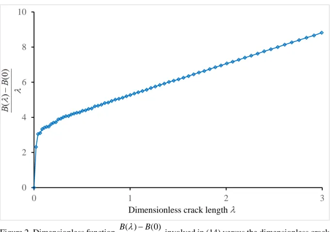
2 inc c 1 1 2 ( ) (0) ( ) with ( ) ( , , ), ( ) d B B G d T G E B E V y y t λ λ λ λ λ ρ θ − = ≥ = Ψ (14)Note that in (14), according to (12), V can be replaced with 1 V . The scaling coefficients ( )ˆ1 B λ are dimensionless and it can be shown that the above inequality is the exact counterpart of the first inequality in (3). The dimensionless function
(
B( )λ −B(0) /)
λ is depicted in Figure 2; it is a strictly increasing function of λ . Since this function is the result of a difference between two terms, both calculated by the path integral (14) after having solved a FE analysis, this introduces inaccuracies and the curve is not as smooth as it could be expected. Note that, releasing double nodes to vary the crack length allows using a unique mesh topology, thus reducing a major source of numerical errors. Anyhow, eqn. (16) (below) can be solved without difficulty.Figure 2. Dimensionless function B( )λ B(0) λ
−
involved in (14) versus the dimensionless crack length λ. 0 2 4 6 8 10 0 1 2 3
The stress condition in (1), using expressions derived from the inner expansion, can be written (taking only into account the tensile component σ ) as:
(
)
(
1)
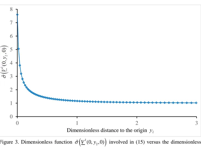
c (0, , 0) (0, , 0) d U l T V σ = σ λ ≥σ (15)Relationship (15) is the counterpart of the second inequality in (3). The dimensionless function
(
1)
2 (0, , 0)
V y
σ is depicted in Figure 3; it is a decreasing function of y (keep in mind that this 2 function is calculated prior to crack nucleation).
Figure 3. Dimensionless function σ
(
V1(0,y2, 0))
involved in (15) versus the dimensionless distance to the origin y2.Discarding T from (14) and (15) leads to a relationship giving the dimensionless crack length at initiation λc (see the analogy with (4)), which is independent of the applied load:
c c c 2 2 c c c 1 ( ) (0) 1 (0, , 0) B B EG L d d λ σ λ λ σ − = = (16)
Then, the actual initiation length is:
c c
l =λd (17)
and the applied load at failure can be derived (to be compared to (6), where d intervenes through λc): 0 1 2 3 4 5 6 7 8 0 1 2 3
c c c (0, , 0) T σ σ λ = (18)
This approach takes advantage of a single computation in the inner domain regardless the shape of the specimen and particularly the depth of the flaw, because all the calculations in the inner domain are independent of the global geometry (especially the flaw depth d, which has been dilated to unity).
Remark: It can easily be shown that:
inc inc inc d ( ) ( ) ( ) ( ) d G l G l G l l G l l = + > (19)
As Ginc( )l is a strictly increasing function of l (Figure 2), at crack nucleation G l( )c >Gc, which means that l is not an arrest length. The crack jumps a length c l and then grows in an unstable c manner. As a consequence, the length l cannot be observed experimentally. c
3. Influence of a surface flaw on the measured strength
3.1 V-notches
Usami et al. (1986) reported an extensive experimental campaign of strength measurements of various ceramics as a function of the size and the shape of different flaws. For illustrative purposes, we have selected only results on alumina (Al2O3, Young’s modulus E =350GPa,
Poisson’s ratio ν =0.3, toughness KIc =3.1 MPa m1/2) to compare with the predictions of the
CC using the asymptotic approach of Section 2.4. The fracture energy G is derived from the c fracture toughness K using Irwin’s relationship under plane strain assumption: Ic
2 2 c Ic 1 G K E ν − = (20)
Figure 4. Tensile strength of alumina. Comparison between experiments (diamonds) and predictions using the asymptotic approach of the CC for a 90 deg. opening sharp notch (red solid line) and a crack like surface flaw (dashed blue line).
As shown in Figure 4, the CC predictions, for a flaw made of a shallow V-notch with opening angle 90 deg. (Figure 1), agree quite well with experiments. In particular, they take into account the smooth transition between an energy driven failure load (on the right) and a stress driven one (on the left). Obviously the intrinsic tensile strength σc to be retained in that case is the left asymptotic value (~ 200 MPa); it is the value that was actually used to make the calculations exhibited in this section. As it will be shown in Section 4, the intrinsic tensile strength depends strongly on the grain size (Danzer et al., 2007), which average is reported to be around 0.02 mm by Usami et al. When the extrinsic flaw size drops below the grain size (commonly admitted as the intrinsic flaw size), it is the grain size that becomes predominant.
The crack-like flaw curve is classically obtained using an expression of the stress intensity factor K at the tip of a short surface crack (Tada et al., 2000): I
I 1.122
K = T πd (21)
The crack growth criterion KI =KIc remains valid as long as T <σc. For the case T ≥σc it is the stress criterion T =σc the one that governs. In this model, the transition occurs for
c 0.06
d = mm, which is slightly larger than the average grain size reported by Usami and likely indicates the presence of coarser grains. However, it is of course not an exact measure because it relies strongly on the crack-like flaw assumption. Note that there exists a controversy on the role of the average grain size vs. the larger grains (Rice, 1997).
Obviously, there is not a big difference between the 90 deg. V-notch and the sharp crack. A comparison with a larger opening 120 deg. is proposed in Figure 5 without revealing a significant difference. 40 400 0.0005 0.005 0.05 0.5 A p p li ed l o ad a t fa il u re ( M P a) Flaw depth (mm)
V-notch - matched asymptotics Crack-like flaw
Figure 5. Tensile strength of alumina. Comparison between experiments (diamonds) and predictions using the asymptotic approach of the CC for various V-notches opening (from 0 deg. to 120 deg.).
3.2 A remark on V-notches
Clearly from (10) and (11), V (and 1 V ) undergoes a singularity at the tip of the V-notch and ˆ1 the Williams expansion reads:
1 1 2
( , ) ( ) ...
V y y = +C κ ραu θ + (22)
Where C is an irrelevant constant, α the singular exponent (Table 1) and ( )u θ the associated mode (Leguillon and Sanchez-Palencia, 1987). Here κ is the dimensionless generalized stress intensity factor (see (Zghal et al., 2018) for a table of values).
Table 1. Mode I singular exponent α vs. the V-notch opening ω.
V-notch opening (deg.) 0 30 90 120 160 180 α 0.5 0.502 0.545 0.616 0.819 1
Using (10), the generalized stress intensity factor k (MPa m1-α) of the actual solution U can d be expressed in terms of the notch depth
1
k =Td −ακ (23)
Then according to Leguillon (2002), if the crack initiation length is small compared to the notch depth (i.e. if the notch depth is large enough while remaining small compared to the specimen size) then the failure initiation criterion can be written as:
40 400 0.0005 0.005 0.05 0.5 A p p li ed l o ad a t fa il u re ( M P a) Flaw depth (mm) 0 deg. 90 deg. 120 deg. Experiments by Usami
1 2 2 1 Ic c c c 1 1 * K k k k T A d α α α σ κ − − − ≥ = ⇒ ≥ (24)
Where A is a scaling coefficient (Leguillon, 2002)(see also (Zghal et al., 2018) for a table of * values of A*). Therefore, when the notch depth increases, the failure load tends towards an asymptote with slope α−1 in the log-log diagrams of Figures 4 and 5. This property has been exploited to extend the curves without additional calculations, i.e without solving (16).
3.3 U-notches
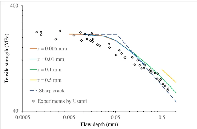
A similar comparison was also conducted with simulations carried out on surface flaws made of a blunted slit (referred to as U-notches) with varying root radii (Figure 6). It is shown that the agreement remains good only for small root radii. Large root radii (e.g. r > 0.1 mm) prevent making calculations for shallow slits, hence the smaller segments of curves in Figure 6.
Figure 6. Tensile strength of alumina. Comparison between experiments (diamonds) and predictions using the asymptotic approach of the CC for a blunted slit with varying root radius (from 0.001 to 0.5 mm).
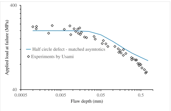
3.4 Semi-circular defect
Among other defect shapes Usami et al. suggest also a semi-circular surface flaw, but again, the matching is not as good as for sharp V-notches, as can be observed in Figure 7. However, it can be noted that differences only occur when the defect size becomes large, otherwise all geometries tend to merge.
40 400 0.0005 0.005 0.05 0.5 T en si le s tr en g th ( M P a) Flaw depth (mm) r = 0.005 mm r = 0.01 mm r = 0.1 mm r = 0.5 mm Sharp crack Experiments by Usami
Figure 7. Tensile strength of alumina. Comparison between experiments (diamonds) and predictions using the asymptotic approach of the CC for a semi-circular surface flaw.
4. A property of the intrinsic tensile strength
4.1 The Petch law
The Petch law describes the influence of the grain size on the strength of a polycrystalline material. It was originally developed for metals where the yield strength was found to be inversely proportional to the square root of the grain size, as dislocations pile up at the grain boundaries, also known as the Hall-Petch law (Hall, 1951; Petch, 1953). Thus it should be better here to talk about a Petch-like law dedicated to tensile strength rather than yield strength. As already mentioned, such an analysis can be carried out only if extrinsic flaws (surface flaws for instance) are smaller than the grain size which is commonly taken as the intrinsic flaw size (Wachtman et al., 2009). In this section we will only consider the so-called “90-notch flaw” corresponding to a V-notch flaw with opening 90 deg.
Usami et al. (1986) reported a small increase of the toughness as the average grain size g decreases. We will use the following empirical approximation derived from their data:
Ic( ) 0.25 ln( ) 4.12
K g = − g + (25)
where g is expressed in µm and K in MPa mIc 1/2.
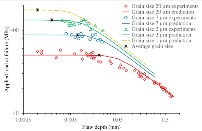
Figure 8 shows a comparison between experiments carried out by Usami et al. (1986) on alumina for different average grain sizes and the predictions using the 90-notch flaw approach and an extrapolation to the limit case. This does not involve new calculations, but only to solve (16) and (18) for new values of G (i.e. c K ) and Ic σc, as reported in Table 2. The intrinsic tensile strength σc (plateau on the left of the solid lines in Figure 8) is an estimate made to serve as guide to the eye. The reported average grain sizes are represented by stars. It is important to
40 400 0.0005 0.005 0.05 0.5 A p p li ed l o ad a t fa il u re ( M P a) Flaw depth (mm) Half circle defect - matched asymtotics Experiments by Usami
point out that these values correspond more or less to the points where the curves become plateaus.
Figure 8. Tensile strength of alumina. Comparison between experiments for different reported average grain size (stars): 0.02 mm (red diamonds), 0.007 mm (blue circles), 0.002 m (green triangles) and predictions using the 90-notch flaw (solid lines of the same color). The gold dashed line corresponds to an extrapolation to the limit case (see Table 2).
The Petch law is often reported (Zimmermann et al., 1998) with two regimes based on the crack-like flaw: (i) the first one described by the Griffith criterion and baptized as Orowan regime, and (ii) a plateau referred to as Petch regime. According to (Chantikul et al., 1990; Danzer et al., 2007) this plateau could appear for high-density alumina around σc=700MPa, and should be taken as the “intrinsic-intrinsic” tensile strength. It is doubly intrinsic because this limit does not depend on the size of either extrinsic defects or intrinsic defects (e.g. grain size). Concurrently, a fracture toughness value of KIc=3.64MPa m1/2 has been reported (25)
and the average grain size g corresponding to the plateau can be roughly estimated to be 0.001 mm (Figure 8). Moreover, solving (16) in this case leads to λc , which means that at 13 nucleation the crack jumps through 13 grains. Table 2 summarizes all these results.
40 400 0.0005 0.005 0.05 0.5 A p p li ed l o ad a t fa il u re ( M P a) Flaw depth (mm)
Grain size 20 µm experiments Grain size 20 µm prediction Grain size 7 µm experiments Grain size 7 µm prediction Grain size 2 µm experiments Grain size 2 µm prediction Grain size 1 µm prediction Average grain size
Table 2. Reported average grain size and toughness from Figure 7 in (Usami et al., 1986) (see eqn. (25)) and estimate of the corresponding intrinsic tensile strength. The last line corresponds to extrapolations according to an intrinsic tensile strength of 700 MPa (Danzer et al., 2007).
Average grain size g (mm) Toughness Ic K (Mpa m1/2) Intrinsic tensile strength σc (MPa) 0.020 3.10 200 0.007 3.34 350 0.002 3.49 530 0.001 3.64 700
The tensile strength versus grain size relation is generally represented as a function of the inverse of the square root of the grain size as in Figure 9. One can point out that the growing part is not strictly linear due to: (i) the approximate values of the average grain sizes and the intrinsic tensile strengths (determined by eye), and/or (ii) the variations of K as a function of Ic the grain size (see (25)). Results by Chantikul et al. (1990) are superimposed. Obviously from their micrographs, the grain size they measured corresponds to the largest grains, thus the retained value for the average grain size is here one half of the measured one according to the Hillert’s rule they refer to (Hillert, 1965).
Figure 9. Tensile strength of alumina. The intrinsic tensile strength (solid blue line and stars) function of the inverse square root of the average grain size, following Zimmermann et al. (1998) nomenclature. Results by Chantikul et al (1990) are superimposed (circles).
The reader's attention is drawn to the notations used in Figures 9 and 12 that could be tiny bit puzzling if not acquainted with. As it is common in some material science communities, the abscissa is expressed as the inverse square root of the grain size.
0 200 400 600 800 0 10 20 30 40 50 In tr in si c te n si le s tr en g th ( M P a)
Average grain size (mm-1/2)
Prediction
Experiments by Chantikul et al.
Orowan regime
4.2 The role of residual stresses
In Figure 9, the plateau is flat whereas many plots exhibit a slight slope in the Petch regime (Chantikul et al., 1990; Harper, 2001). An explanation might be the presence of internal thermal residual stresses, associated with the random distribution of grains that have direction dependent coefficients of thermal expansion as well as elastic properties. Vedula et al. (2001) reported that the highest principal stress could be as large as ∼530 MPa for a cooling temperature ∆ = −T 1500°C.
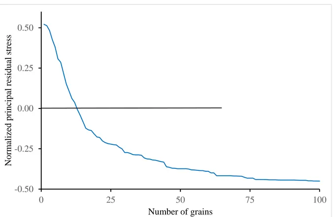
A simple simulation has been performed to estimate the role of residual stresses. First, the largest principal stress is supposed to be randomly distributed in each grain (a set of 10000 grains was used for 10 different random selections); it is parametrized by its largest value in the specimen. In a next step all these values are projected onto a single direction (that of the crack, itself random with respect to the basis chosen to rotate the grains). Then neighboring values (to simulate neighboring grains) are gathered 2 by 2, 3 by 3 and so on. For a grouping j by j , each family f is characterized by the smaller residual stress over the family, and the maximum j is taken over all the families and finally averaged (upper bar) over the 10 random selections as:
( ) max min ( ) j j j i i f f σ σ ∈ = (26)
If only one grain is broken, it promotes the failure of the grain where the largest residual stress lies. If two grains are broken simultaneously, of all pairs of grains, the one where the smaller of the two residual stresses is the largest has to be searched for. Failure of this pair will be promoted by the residual stresses. And so on with 3 grains and j grains. Finally, as it is a random distribution of residual stresses, it is averaged over 10 of trials. As a consequence σ( )j is the (normalized) residual stress to take into account if j neighboring grains are broken simultaneously, being the most favourable value for fracture of j grains. Note that σ(1) is the largest value reached by the residual stresses, it differs from 1 due to the projection. This is illustrated in Figure 10.
Figure 10. The normalized thermal residual stress resulting from a random distribution through the grains, function of the number of grains broken simultaneously.
It has been mentioned in the previous section that for g =0.001mm, the crack jumps 13 grains at nucleation. It is worth mentioning that σ(13) , as a consequence, the thermal residual 0 stresses have no influence on the transition point between Orowan and Petch regimes. Solving (16) for decreasing values of the grain size g , and taking into account the corresponding fracture properties reported in Table 2, we obtain the number of grains broken simultaneously at crack initiation as a function of the grain size, as shown in Figure 11. Combining Figure 10 and Figure 11, i.e. taking into account the thermal residual stresses within the grains in the Petch regime, leads to Figure 12, representing the intrinsic tensile strength versus average grain size for different values of maximum residual principal stresses. Note that the Orowan regime part has been smoothed compared to Figure 9. The slope is often reported as K , but keep in mind Ic that this parameter slightly varies with the grain size according to (25). Otherwise, it is almost unchanged because crack initiation is mainly driven by the energy condition in the Orowan regime.
There may obviously be other causes that create this slope. For instance, Wachtman et al. (2009) mentioned for example that “finer grains have lower concentrations of impurities along the grain boundaries and, therefore, may be stronger”, but such considerations are beyond the scope of this work. -0.50 -0.25 0.00 0.25 0.50 0 25 50 75 100 N o rm al iz ed p ri n ci p al r es id u al s tr es s Number of grains
Figure 11. Number of grains broken simultaneously at crack initiation, function of the grain size.
Figure 12. Tensile strength of alumina. The intrinsic-intrinsic tensile strength (Petch regime) as a function of the inverse square root of the average grain size for different values of the largest residual principal stress: 0 MPa (red), 100 MPa (blue), 300 MPa (green) and 500 MPa (gold).
0 10 20 30 40 0 0.0002 0.0004 0.0006 0.0008 0.001 0.0012 N um be r of gr ai ns
Average grain size (mm)
0 250 500 750 1000 0 10 20 30 40 50 60 In tr in si c te n si le s tr en g th ( M P a)
Average grain size (mm-1/2)
Orowan regime
Max. residual stress 0 MPa Max. residual stress 100 MPa Max. residual stress 300 MPa Max. residual stress 500 MPa
Petch regime
5. Conclusion
The main goal of the present analysis was to provide a satisfying definition of the tensile strength of a ceramic to be used in numerical models for prediction of crack initiation. Based on experiments by Usami et al. (1986) on alumina, it has been shown that the appropriate value to be considered corresponds to the plateau observed when the size of the extrinsic flaws (defects due to manufacturing or deliberately created for experimental purpose) becomes smaller than the average grain size. This is the only way for the numerical models, we focused herein on the CC but it is known that CZM’s give similar result (Cornetti et al., 2016; Martin et al., 2016), to recover the experiments measuring the strength as a function of the flaw size. Of course, more classically, it works for larger geometric perturbation, such as V-notches made for experimental purpose which act like major flaws. This value, so-called intrinsic tensile strength, depends on the grain size. It is totally deterministic as opposed to the extrinsic strength that is governed by Weibull's statistics. This conclusion has an important consequence for future works: if tests on V-notched or U-notched specimens make it possible, using the CC, to determine a tensile strength, then the value thus obtained will be the intrinsic strength. This approach avoids all discussion on stochastic aspects.
Furthermore, it has been observed, in experiments by Danzer et al. (2007), that these plateaus have also a limit as the grain size decreases, the so-called intrinsic-intrinsic tensile strength. Then using the CC, it has been possible to recover a Petch-like law for brittle polycrystalline materials. In the limit case, baptized as Petch regime, the CC predicts that an increasing numbers of grains will simultaneously be broken at the stage of crack initiation as the grain size decreases. As a consequence, the microscopic internal stresses due the anisotropy of the grains may also influence the intrinsic strength of the material in this regime.
References
Bermejo R., Danzer R., 2014. Mechanical characterization of ceramics: Designing with brittle materials. In Comprehensive hard materials, vol. 2, Elsevier Ltd, Oxford, 285-298.
Bermejo R., Supancic P., Krautgasser C., Morrell R., Danzer R., 2013. Subcritical crack growth in Low Temperature Co-fired Ceramics under biaxial loading. Engng. Fract. Mech. 100, 108-121.
Carniglia S.C., 1965. Petch relation in single-phase oxide ceramics. J. Am. Ceram. Soc. 48, 580-583.
Carniglia S.C., 1972. Reexamination of experimental strength-vs-grain-size data for ceramics. J. Am. Ceram. Soc. 55, 243-249.
Chantikul P., Bennison S.J., Lawn B.R., 1990. Role of grain size in the strength and R-curve properties of alumina. J. Am. Ceram. Soc. 73, 2419-2427.
Cornetti P., Sapora A., Carpinteri A., 2016. Short cracks and V-notches: Finite Fracture Mechanics vs. Cohesive Crack Model. Engng. Fract. Mech. 168, 2-12.
Cornetti P., Taylor D., Carpinteri A., 2010. An asymptotic matching approach to shallow-notched structural elements. Engng. Fract. Mech. 77, 348-358.
Damani R., Gstrein R., Danzer R., 1996. Critical notch root radius effect in SENB-S fracture toughness testing. J. Eur. Ceram. Soc. 16, 695-702.
Danzer R., 2014. On the relationship between ceramic strength and the requirements for mechanical design. J. Eur. Ceram. Soc. 34, 3435-3460.
Danzer R., Harrer W., Supancic P., Lube T., Wang Z., Börger A., 2007. The ball on three-ball test – Strength and failure analysis of different materials. J. Eur. Ceram. Soc. 27, 1481-1485. Doitrand A., Leguillon D., 2018. 3D application of the coupled criterion to crack initiation
Elices M., Guinea G.V., Gomez J., Planas J., 2002. The cohesive zone model: advantages, limitations and challenges. Engng. Fract. Mech. 69, 137-163.
Freiman S.W., 2013. Environmentally enhanced fracture of glasses and ceramics. In Handbook of advanced ceramics (second edition), Ed. S. Somiya, Academic Press, 753-764.
Griffith A.A., 1921. The phenomena of rupture and flow in solids. Phil. Trans. Of the Royal Soc. of London - Series A 221, 163-198.
Hall, E.O., 1951. The deformation and ageing of mild steel: III Discussion of results. Proc. Phys. Soc. B 64, 747-753.
Harper C., 2001. Handbook of ceramics, glasses and diamonds. Mc Graw-Hill, New York. He M.Y., Turner M.R., Evans A.G., 1995. Analysis of the double cleavage drilled compression
specimen for interface fracture energy measurements over a range of mode mixities. Acta Metal. Mater. 43, 3453-3458.
Hillert, M., 1965. On the theory of normal and abnormal grain growth. Acta Metall., 13, 227-238.
Irwin G., 1958. Fracture. Hand. der Physic, Springer, Berlin, vol. VI.
ISO 18756, 2008. Fine ceramics (advanced ceramics, advanced technical ceramics)- determination of fracture toughness of monolithic ceramics at room temperature by the surface crack in flexure (SCF) Method.
ISO 23146, 2008. Fine ceramics (advanced ceramics, advanced technical ceramics)- Test methods for fracture toughness of monolithic ceramics – Single-edge V-notch beam (SEVNB) method.
Krautgasser C., Chlup Z., Supancic P., Danzer R., Bermejo R., 2016. Influence of subcritical crack growth on the determination of fracture toughness in brittle materials. J. Eur. Ceram. Soc. 36, 1307-1312.
Leguillon D., 2002. Strength or toughness? A criterion for crack onset at a notch. Eur. J. of Mechanics – A/Solids, 21, 61-72.
Leguillon D., 2011. Determination of the length of a short crack at a v-notch from a full field measurement. Int. J. Solids Structures 48, 884-892.
Leguillon D., 2013. A simple model of thermal crack pattern formation using the coupled criterion. C. R. Mécanique, 341, 538-546.
Leguillon D., 2014. An attempt to extend the 2D coupled criterion for crack nucleation in brittle materials to the 3D case. Theor. Appl. Fract. Mech., 74, 7-17.
Leguillon D., Sanchez-Palencia E., 1987. Computations of Singular Solutions in Elliptic Problem and Elasticity. John Wiley, New-York and Masson, Paris.
Leguillon D., Quesada D., Putot C., Martin E., 2007. Size effects for crack initiation at blunt notches or cavities. Engng. Fract. Mech. 74, 2420-2436.
Leguillon D., Martin E., Lafarie-Frenot M.C., 2015. Flexural vs. tensile strength in brittle materials. C.R. Mécanique 343, 275-281.
Leguillon D., Sanchez-Palencia E., 1987. Computation of singular solutions in elliptic problems and elasticity, John Wiley & Son, New York and Masson, Paris.
Martin E., Leguillon D., 2004. Energetic conditions for interfacial failure in the vicinity of a matrix crack in brittle matrix composites. Int. J. Solids Structures, 41, 6937-6948.
Martin E., Vandellos T., Leguillon D., Carrère N., 2016. Initiation of edge debonding: Coupled criterion versus cohesive zone model. Int. J. Fract. 199, 157-168.
Zghal J., Moreau K., Moes N., Leguillon D., Stolz C., 2018. Analysis of the failure at notches and cavities in quasi-brittle media using the Thick Level Set damage model and comparison with the coupled criterion. Int. J. Fract., https://doi.org/10.1007/s10704-018-0287-6
Petch, N.J., 1953. The cleavage strength of polycrystals. J. Iron Steel Inst., 174, 25-28.
Rice R.W., 1997. Review. Ceramic tensile strength - grain size relations: grain sizes, slopes, and branch intersections. J. Mater. Sci. 32, 1673-1692.
Strobl S., Lube T., Supancic P., Schöppl O., Danzer R., 2017. Surface strength of balls made of five structural ceramic materials evaluated with the Notch Ball test (NBT). J. Eur. Ceram. Soc. 37, 5065-5070.
Strobl S., Rasche S., Krautgasser C. Sharova E., Lube T., 2014. Fracture toughness testing of small ceramic disks and plates. J. Eur. Ceram. Soc. 34, 1637-1642.
Tada H., Paris P.C., Irwin G.R., 2000. The Stress Analysis of Cracks Handbook. Third edition, ASME Press, New York.
Tanné E., Li T., Bourdin B., Marigo J.J., Maurini C., 2018. Crack nucleation in variational phase-field models of brittle fracture. J. Mech. Phys. of Solids 110, 80-99.
Taylor D., 2007. The theory of critical distance. Elsevier, Amsterdam.
Usami S., Kimoto H., Takahashi I. and Shida S., 1986. Strength of ceramic materials containing small flaws. Engng. Fract. Mech. 23, 745-761.
Van Dyke M., 1964. Perturbation methods in fluid mechanics. Academic Press, New York.
Vedula V.R., Glass S.J., Saylor D.M., Rohrer G.S., Carter W.C., Langer S.A., Fuller Jr E.R., 2001. Residual-stress predictions in polycrystalline alumina. J. Am. Ceram. Soc. 84, 2947-2954.
Wachtman J.B., Cannon W.R., Matthewson M.J., 2009. Mechanical properties of ceramics. Second edition, John Wiley, New York.
Weibull W., 1951. A statistical distribution function of wide applicability. J. Appl. Mech. 18, 293–297.
Weissgraeber P., Leguillon D., Becker W., 2016. A review of Finite Fracture Mechanics: Crack initiation at singular and non-singular stress-raisers. Arch. Appl. Mech. 86, 375-401.
Zimmermann A., Hoffman M., Flinn B.D., Bordia R.K., Chuang T.J., Fuller Jr E.R., Rödel J., 1998. Fracture of alumina with controlled pores. J. Am. Ceram. Soc. 81, 2449-2457.