Analytics for online markets

(1)

Analytics for Online Markets

by

Kris Johnson

B.S., Georgia Institute of Technology (2007)

Submitted to the Sloan School of Management

in partial fulfillment of the requirements for the degree of

Doctor of Philosophy in Operations Research

at the

MASSACHUSETTS INSTITUTE OF TECHNOLOGY

June 2015

c

○ Massachusetts Institute of Technology 2015. All rights reserved.

Author . . . .

Sloan School of Management

May 5, 2015

Certified by. . . .

David Simchi-Levi

Professor of Engineering Systems Division and the

Department of Civil and Environmental Engineering

Thesis Supervisor

Accepted by . . . .

Dimitris Bertsimas

Boeing Professor of Operations Research

Co-director, Operations Research Center

(2)

(3)

Analytics for Online Markets

by

Kris Johnson

Submitted to the Sloan School of Management on May 5, 2015, in partial fulfillment of the

requirements for the degree of

Doctor of Philosophy in Operations Research

Abstract

Online markets are becoming increasingly important in today’s world as more people gain access to the internet. Furthermore, the explosion of data that is collected via these online markets provides us with new opportunities to use analytics techniques to design markets and optimize tactical decisions. In this thesis, we focus on two types of online markets -peer-to-peer networks and online retail markets - to show how using analytics can make a valuable impact.

We first study scrip systems which provide a non-monetary trade economy for exchange of resources; their most common application is in governing online peer-to-peer networks. We model a scrip system as a stochastic game and study system design issues on selection rules to match trade partners over time. We show the optimality of one particular rule in terms of maximizing social welfare for a given scrip system that guarantees players’ incentives to participate, and we investigate the optimal number of scrips to issue under this rule.

In the second part, we partner with Rue La La, an online retailer in the online flash sales industry where they offer extremely limited-time discounts on designer apparel and acces-sories. One of Rue La La’s main challenges is pricing and predicting demand for products that it has never sold before. To tackle this challenge, we use machine learning techniques to predict demand of new products and develop an algorithm to efficiently solve the subse-quent multi-product price optimization. We then create and implement this algorithm into a pricing decision support tool for Rue La La’s daily use. We conduct a controlled field experiment which estimates an increase in revenue of the test group by approximately 10%. Finally, we extend our work with Rue La La to address a more dynamic setting where a retailer may choose to change the price of a product throughout the course of the selling season. We have developed an algorithm that extends the well-known multi-armed bandit algorithm called Thompson Sampling to consider a retailer’s limited inventory constraints. Our algorithm has promising numerical performance results when compared to other algo-rithms developed for the same setting.

Thesis Supervisor: David Simchi-Levi

Title: Professor of Engineering Systems Division and the Department of Civil and Environmental Engineering

(4)

(5)

Acknowledgments

First and foremost, I would like to thank my advisor, David Simchi-Levi. I couldn’t have imagined a better advisor and mentor to help guide me through my PhD. David always believed in me and helped me achieve things that I didn’t even think were possible. He has taught me how to be an effective researcher and the art of guiding research projects from start to finish. Not only was David an excellent academic advisor, but he also truly cares about my happiness and success. His help and advice has been invaluable, and I am so lucky to have him as my advisor.

I would also like to thank my thesis committee members, Asu Ozdaglar and Steve Graves, for their time and help guiding my PhD work to completion and supporting my goal of becoming a professor. I had the chance to take Asu’s excellent game theory class early in my PhD studies, and her class helped shape Chapter 2 of this thesis. I had the pleasure of being Steve’s teaching assistant for a couple of semesters and really enjoyed working with and learning from him.

Two other faculty members that have mentored me are Joel Sokol (Georgia Tech) and Rob Freund (MIT), and I would like to thank them both for their time and support. I am so thankful to have worked with Joel at Georgia Tech; he opened my eyes to the possibility of pursuing a PhD in operations research and without him, I certainly would not be at MIT today! I am also fortunate to have worked as Rob’s teaching assistant at MIT. Both Rob and Joel are fantastic teachers, and both have made themselves available and proactively reached out to offer advice and mentorship to help me navigate the academic world.

I appreciate the Operations Research Center faculty and staff for supporting me through-out this journey. The ORC co-directors, Dimitris Bertsimas and Patrick Jaillet, have done a great job guiding the ORC over the years. The ORC staff, Laura Rose and Andrew Carvalho, have made everything run so smoothly. Furthermore, I’d like to thank Janet Kerrigan who is always willing to lend a helping hand and never fails to make me laugh.

I am so fortunate to have made such amazing friends during my time at MIT: Fernanda Bravo, Andre Calmon, Maxime Cohen, Iain Dunning, Adam Elmachtoub, David Fagnan, Swati Gupta, Vishal Gupta, Nathan Kallus, Angie King, Alex Lee, Ben Letham, Will Ma,

(6)

Velibor Misic, Allison O’Hair, Leon Valdes, He Wang, Yehua Wei, Alex Weinstein, and Nataly Youssef. Your friendship and support have made the last five years the best years of my life - thank you! Special thanks to Angie and Fernanda, who have become two of my closest friends ever since we survived the first year of classes together. We have traveled the world together and they have always been a huge source of support. In addition, I’d like to thank David Ward, Ashleigh and Brad Range, and Mary Winn and Martin Miller for their friendship and support in Boston over the last several years and reminding me that there is, in fact, life outside of MIT.

I am also lucky to have collaborated with wonderful people on the work presented in this thesis, each of whom will be a lifelong friend. Chapter 2 was done in close collaboration with Peng Sun, a professor at Duke University who has really coached me to be a productive researcher. The work in Chapter 3 was done in partnership with the online retailer Rue La La, and I am very grateful to have worked with Murali Narayanaswamy, VP of Marketing & Strategy at Rue La La, and Alex Lee; I also thank the numerous other Rue La La and Accenture executives and employees for their assistance and support throughout our project. In the last year, I am so thankful to have had the opportunity to work with He Wang (Chapter 4) who is a brilliant researcher and has become a great friend.

Last but certainly not least, I would like to thank my family - Sharon Johnson (mom), Tom Johnson (dad), Kate Fuchs (sister), and Dan Ferreira (fiancé). Without them, I would certainly not be graduating from MIT today. Dan was one of the first people to encourage me to pursue my PhD and has been incredibly supportive of me throughout the ups and downs of this journey; I’m so lucky to spend the rest of my life with him. Kate has been my best friend since Day 1, and she has also been a role model of how to achieve balance between academics, work, and personal life; I’m so fortunate to have her as my twin sister. Finally, I owe my deepest gratitude to my parents. Words cannot describe how amazing my parents are and how appreciative I am of their lifetime of love, support, and encouragement. They instilled the value of education and love for learning in me at a very young age. They have always believed in me, even when I did not, and their love and support have lifted me to heights that I did not think were possible. Mom and dad, I dedicate this thesis to you.

(7)

List of Figures

2-1 Probability of no trade with 𝑁 = 3 players. . . 25

2-2 Conditions (2.13) and (2.15), with 𝑁 = 5. . . 35

2-3 The non-monotone, unimodal structure of the value function in its minimum recurrent state. . . 37

3-1 Example of three events shown on Rue La La’s website . . . 48

3-2 Example of three styles shown in the men’s sweater event . . . 48

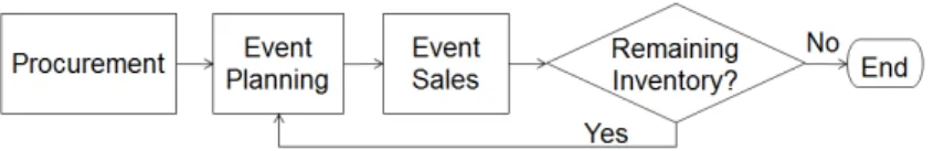
3-3 Subset of Rue La La’s procure-to-pay process . . . 49

3-4 First exposure (new product) sell-through distribution by department . . . . 50

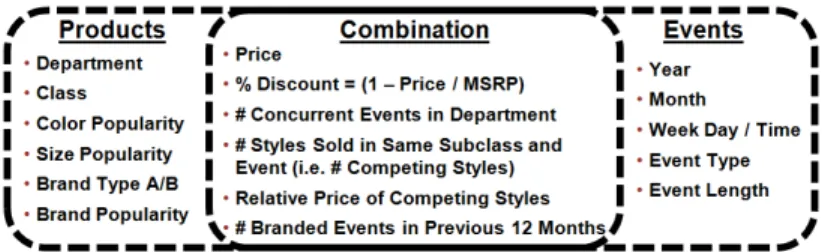
3-5 Summary of features used to develop demand prediction model . . . 56

3-6 Description of select features . . . 56

3-7 Demand curves (percent of total sales by hour) for 2-day events . . . 59

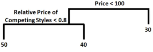
3-8 Transforming unconstrained demand prediction (ˆ𝑢𝑖) to sales prediction ( ˆ𝑑𝑖) . 60 3-9 Illustrative example of a regression tree . . . 61

3-10 Architecture of pricing decision support tool . . . 72

4-1 Performance comparison of dynamic pricing algorithms . . . 98

B-1 Cluster dendrogram for 2-day events . . . 131

B-2 Performance evaluation of demand unconstraining approach . . . 133

C-1 Performance results comparison of regression models . . . 137

C-2 Comparison of MAE and MAPE . . . 138

(10)

(11)

List of Tables

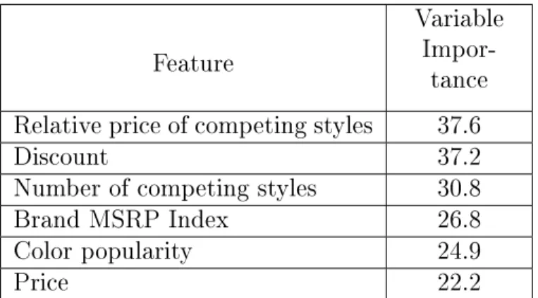
3.1 Features with largest variable importance . . . 63 3.2 Example of LP Bound Algorithm performance . . . 69 3.3 Percent increase in each treatment group’s metric over the control group’s

metric . . . 74 3.4 Wilcoxon rank sum test results for the impact on sell-through . . . 78 3.5 Estimate of additive increase in percent of available revenue earned due to

raising prices . . . 79 3.6 Estimate of percent increase in revenue due to raising prices . . . 81 4.1 Literature on dynamic learning and pricing with limited inventory . . . 90 C.1 Descriptive statistics of the test data set for Rue La La’s largest department 135 C.2 Performance metrics used to compare regression models . . . 136

(12)

(13)

Chapter 1 Introduction

Online markets are becoming increasingly important as more people around the world gain internet access. As of April 1, 2015, there were nearly 3.1 billion internet users around the world; within the United States alone, nearly 90% of the population now has internet access [Internet Live Stats, 2015]. In this thesis, we focus on two types of online markets: peer-to-peer networks and online retail markets. Peer-to-peer networks refer to a network of computers such that each computer can act as a server for the others; peer-to-peer networks are most commonly used as online file sharing systems, which in 2014 accounted for over 5% of peak period internet traffic in North America [Statista, 2015]. Online retail markets refer to retailers who only sell products online (e.g. Amazon.com); this industry has experienced approximately 10% annual growth over the last 5 years in the United States, reaching nearly $300B in revenue in 2014 [Lerman, 2014].

Peer-to-peer networks and online retail markets have faced a variety of challenges that are rather unique to online markets as compared to their offline counterparts. For example, implementations of many peer-to-peer file sharing systems have failed due to system design issues such as having a lack of incentives for users to share files; with no governing body in place to manage these systems and user participation, users can easily take advantage of these networks and download files without sharing any of their own. As another example, online retailers have additional information available to them compared to brick-and-mortar stores; one challenge they face is in harnessing this data to make tactical pricing decisions that maximize revenue. We employ a variety of data-driven, analytics techniques - such as

(14)

regression, clustering, reinforcement learning, and optimization - to address these system design and tactical challenges that online markets face.

In the first part of this thesis, we design a "scrip system" that can be used to govern peer-to-peer networks and align incentives of users to both receive and provide files. A "scrip system" is simply a market that uses "scrips", or coupons, instead of currency to exchange goods and services. The use of scrip systems in the past has been limited, most likely due to system design issues resulting in market crashes. In our work, we aim to design scrip systems that avoid these market crashes, hence allowing their use in governing the operations of peer-to-peer networks as well as a variety of other markets. We model a scrip system as an infinite-horizon stochastic game and study system design issues. We show the optimality of one particular rule to maximize social welfare while guaranteeing players’ incentives to participate. We also investigate the optimal number of scrips to issue under this rule. We show that there is an upper bound on the number of scrips allowed in the system, which increases with the time discount factor as well as the ratio between the benefit and cost of service. This work is detailed in Chapter 2.

In the second part of this thesis, we worked in partnership with the online retailer Rue La La to help them use their available data to make tactical pricing decisions that maxi-mize revenue. Rue La La is in the online fashion sample sales industry, where they offer extremely limited-time discounts on designer apparel and accessories. One of the retailer’s main challenges is pricing and predicting demand for products that it has never sold be-fore, which account for the majority of sales and revenue. To tackle this challenge, we use machine learning techniques to estimate historical lost sales and predict future demand of new products. The nonparametric structure of our demand prediction model, along with the dependence of a product’s demand on the price of competing products, pose new challenges on translating the demand forecasts into a pricing policy. We develop an algorithm to ef-ficiently solve the subsequent multi-product price optimization that incorporates reference price effects, and we create and implement this algorithm into a pricing decision support tool for Rue La La’s daily use. We conduct a controlled field experiment and find that sales does not decrease due to implementing tool recommended price increases for medium and high price point products. Finally, we estimate an increase in revenue of the test group by

(15)

approximately 10% with an associated 90% confidence interval of [3%, 18%]. This work is detailed in Chapter 3.

In the third part of this thesis, we extend our work with Rue La La to address a more dynamic setting where a retailer may choose to change the price of a product throughout the course of the selling season. The goal of this work is to develop a dynamic pricing strategy that uses real-time data available in online retail markets to learn unknown demand and then exploit this knowledge to maximize revenue over the remainder of the selling season. The multi-armed bandit problem has been a well-studied formulation of this dynamic pricing problem given unlimited inventory of a product. A classical machine learning algorithm for the multi-armed bandit problem is known as Thompson Sampling, which has been shown to be a highly competitive algorithm in empirical studies and has strong theoretical performance bounds. Many retailers, though, face limited inventory constraints which must be consid-ered when developing a dynamic pricing strategy. Thus, we have developed an algorithm that extends the Thompson Sampling algorithm to consider a retailer’s limited inventory constraints. Our algorithm has promising numerical performance results when compared to other algorithms developed for the same setting. This work is detailed in Chapter 4.

Chapters 3 and 4 represent a departure from the traditional revenue management litera-ture, where demand is often modeled as a parametric function of price. One probable reason for the popularity of these demand functions is their set of properties, such as linearity, con-cavity and increasing differences, that leads to simpler, tractable optimization problems in operations management. On the other hand, data-driven analytics (i.e. “machine learning”) techniques have proven to be very valuable in a variety of fields, and in Chapters 3 and 4 we illustrate how we have used and adapted these analytics techniques to the field of revenue management. With more and more data being collected by online retailers, we show how companies can harness this data to make better pricing decisions.

(16)

(17)

Chapter 2 Analyzing Scrip Systems

2.1 Introduction

Scrips are coupons that are used in place of currency to exchange goods and services; typ-ically, they cannot be exchanged for money, and therefore their sole use is for the good or service which they are intended for. In this chapter we study scrip systems, which are mar-kets that use scrips rather than money to exchange goods and services. Such marmar-kets are typically implemented when the use of governmental currency is impractical or undesirable. One example of a scrip system is that of the Capitol Hill babysitting co-op, documented in [Sweeney and Sweeney, 1977]. A group of about 150 married couples with children who lived in the Washington, D.C. area were tired of looking for and hiring babysitters to watch their children every time they wanted to enjoy a night out, so they decided to join together to form a babysitting co-op, managed by a scrip system. Every couple in the co-op was given an initial amount of coupons, or scrips, to pay for babysitting service by another couple in the co-op who was willing to provide the service. Free riding was mitigated in the system since a couple could only enjoy the service when they had coupons, and earning coupons required providing services.

It turns out that this babysitting co-op experienced market crashes similar to many other types of markets. Initially, they distributed too few coupons and trade rarely occurred. This was likely because either a couple ran out of coupons to pay for service or they hoarded the few coupons for later special situations. In order to solve this issue, the group collectively

(18)

decided to give every couple additional coupons, to the point that each couple valued one additional coupon too little, and therefore was not willing to provide services to earn an additional coupon. This story was popularized by [Krugman, 1999], who related the scrip system’s crashes to economic slumps and monetary policies. Since crashes occurred due to having the wrong number of scrips in the system, a natural and important question to ask is, therefore, what is the “right” number of scrips in a system?

There are many other examples of scrip systems that have been implemented in resource exchange environments, such as online peer-to-peer systems, to prevent free riding (see, e.g., [Vishnumurthy et al., 2003], [Gupta et al., 2003], [Ioannidis et al., 2003], [Sirivianos et al., 2007], [Peterson and Sirer, 2009], [Belenkiy et al., 2007], and [Satoshi Nakamoto, 2009]). The idea is similar to that of the babysitting co-op example, where scrips are credited to users who provide products/services (e.g., share files) and debited when users receive them (e.g., access other’s files), so that in the long-run, the amount of products/services participants can receive matches what they provide.

Other common uses of scrip systems include online resource allocation environments; for example, grid computing networks (see, e.g., [Brunelle et al., 2006]), research testbeds (see, e.g., [Chun et al., 2005], [AuYoung et al., 2007] and [AuYoung et al., 2007]), distributed database systems ( [Stonebraker et al., 1996]), and privacy-enhancing technologies, where a volunteer network of servers are needed to route Internet traffic in order to conceal the user’s IP address ( [Humbert et al., 2011]). Some scholars suggest that the academic journal refereeing process may also be managed by a scrip system!

Clearly scrip systems are important in a variety of settings, yet there has been relatively little work done to analyze their behavior. In all of these examples, the number of scrips in-jected into the system is a determinant of system performance. As seen from the babysitting co-op example, having too few or too many scrips in the system can cause market crashes. Another important question arises in the online applications of scrip systems – how should the service provider be chosen? In this chapter, we analyze a class of scrip systems and provide insights regarding system design: the way service providers should be selected as well as the optimal number of scrips that should be used in the system.

(19)

system in terms of maximizing social welfare, i.e., total utility of all players in the system over time, while making sure that players have the incentive to follow the rules of the scrip system. For scrip systems where the time discount factor is close enough to 1, or trade benefits one partner much more than it costs the other, the maximum social welfare is always achieved no matter how many scrips are in the system. As a result, system optimal performance can be achieved under individual incentive constraints. When the benefit of trade and time discount are not sufficiently large, on the other hand, injecting more scrips in the system hurts most participants; in this case, there is an upper bound on the number of scrips allowed in the system, above which some players may default. We show that this upper bound increases with the discount factor as well as the ratio between the benefit and cost of service.

In the remainder of this section, we provide a literature review on the modeling and analysis of scrip systems. The basics of our model, as well as the optimal centralized control policy, are introduced in Section 2.2. We then study the stochastic game played in the absence of a central planner in Section 2.3 and demonstrate that the central optimal solution can be achieved in the game when the discount factor is sufficiently large. Section 2.4 investigates the impact of the number of scrips in the system. Finally, Section 2.5 concludes the chapter with a summary of our results and potential areas for future work.

2.1.1 Literature Review

As mentioned before, in the computer science literature, several papers have been written regarding the application of scrip systems and their implementation. There have been, however, only a few papers that formally model and analyze scrip systems. [Aperjis and Johari, 2006] is one of the earliest papers that studies a peer-to-peer file sharing system as an exchange economy. They propose a static game where users decide uploading/downloading rates, and they study the market clearing prices in equilibrium. The papers that are most closely related to ours are [Friedman et al., 2006], [Kash et al., 2007], [Kash et al., 2012a] and [Kash et al., 2012b]. In fact, this stream of papers motivated our study.

[Friedman et al., 2006] is one of the first papers that analyzed players’ strategies as well as design characteristics of scrip systems in a stochastic setting. Their model considers a homogeneous population of players in a scrip system with a finite number of scrips. Services

(20)

are provided at a fixed price (in terms of the number of scrips) and incur a fixed and identical utility gain (loss) to each player receiving (providing) the service. They consider an infinite time horizon game with discounting. In each period, a player is chosen uniformly at random to request service, while all other players have the option to volunteer as a service provider, one of whom is selected randomly. Our model, described in Section 2.2, is similar to their model with one major departure. Instead of having a player chosen randomly to provide service, we allow the system designer to choose a service provider selection rule for all players to follow; then we determine the number of scrips that should be injected in the system accordingly. At the end of our analysis, we return to their assumption of randomly selecting a service provider, and we show similar results regarding the number of scrips that should be injected into such a scrip system.

A key assumption adopted in [Friedman et al., 2006] is that each player chooses to volunteer to provide service following a threshold strategy. That is, a player is willing to volunteer to provide service only if his scrip stock is lower than a threshold number of scrips. The paper shows that when the discount factor is close enough to one, there exists an 𝜖-Nash Equilibrium in which each player follows such a threshold strategy. One implication of the threshold strategy is that there exists a total threshold number of scrips in the system, above which no trade occurs and therefore the system will experience a market crash. Our model, on the other hand, does not restrict players’ strategies to be of threshold type; rather, we show the existence of a total threshold number of scrips as a result. Follow-on work in [Kash et al., 2012b] shows that social welfare increases as the number of scrips in the system increases up to this threshold of total scrips, after which the social welfare drops to zero due to the market crash. [Kash et al., 2012a], where the model is further generalized to include multiple player types, characterizes each player’s threshold that achieves the optimal social welfare. In [Kash et al., 2012b], the authors further analyze the impact of altruists and hoarders in the scrip system.

Motivated by the application of scrip systems to privacy-enhancing technologies, [Hum-bert et al., 2011] analyzes scrip systems where each service request requires 𝑛 providers to satisfy. This model directly extends the model in [Kash et al., 2007] to require 𝑛 service providers instead of one. The authors show similar results to those in [Kash et al., 2007]

(21)

in-cluding the existence of an 𝜖-Nash Equilibrium where all players act according to a threshold policy.

Finally, recent literature in economics also studies scrip systems, motivated by the babysit-ting co-op, as the micro-foundation of monetary policy. [Hens et al., 2007] provides an overview of this line of work. There are quite a few differences between their model and ours. The main difference is that they assume no cost to provide service, while we assume providing service incurs a negative utility, and the ratio between the benefit and cost of service plays an important role in our model. Similar to [Friedman et al., 2006], [Hens et al., 2007] also focuses on the random service provider selection rule, which is, one may argue, simple and realistic in many economic settings.

2.2 Basic Model Description

Consider an economy with a non-empty set 𝑁 of players. Each player 𝑖 ∈ 𝑁 has 𝑟𝑖 scrips,

where we abuse notation to use 𝑁 to represent the number of players as well. In each time period, one player at random will be the “service requester” with probability 1/𝑁, and all other players’ types are 0. In any given period, the service requester is able to obtain utility 𝑢 if the player chosen as a service provider (one of the type 0 players) is willing to sacrifice utility 𝑐 < 𝑢 in exchange for 1 scrip and if the service requester has a scrip and is willing to pay 1 scrip for service. Assume a time discount factor 𝛾 for the system.

Denote the “state” of the system to be 𝑠 = (𝑟, 𝑗), where 𝑟 is the vector of scrip stocks (𝑟𝑖)𝑖∈𝑁 and 𝑗 is the service requester. Thus, the total number of scrips in the system is

𝑅 =∑︀

𝑖𝑟𝑖, which does not change over time. “State space” 𝑆 is the collection of all possible

states 𝑠. We denote a stationary policy 𝜋 to map the state (𝑟, 𝑗) into a probability distribution on the remaining players other than 𝑗. The purpose of 𝜋 is to select a service provider for any possible state 𝑠. Denote set Π to represent the set of admissible policies.

At this point it is worth introducing a particular service provider selection rule in Π, the “minimum scrip selection rule” ¯𝜋, where in each round, the type 0 player with the least number of scrips is selected as the service provider. If more than one type 0 player has the fewest scrips, one player is chosen randomly from them with equal likelihood to be the

(22)

service provider. Another example of a selection rule in Π is the “random provider selection rule”, a common selection rule considered in previous literature, where a player is selected as the service provider uniformly at random, independent of her scrip stock.

We first demonstrate that the minimum scrip selection rule, ¯𝜋, maximizes social welfare among all policies in Π in a central planner setting, where we assume that a hypothetical central planner not only chooses the service provider, but also decides whether trade should occur.

2.2.1 Central Planner Setting

Now we consider a hypothetical central planner who tries to maximize the total social welfare over an infinite time horizon with discount factor 𝛾 ∈ (0, 1). In each period, given state (𝑟, 𝑗), the central planner decides whether trade should occur when player 𝑗 has at least one scrip, and if so, chooses a player 𝑖 to be the service provider. Let 𝑒𝑘 be a vector in ℜ𝑁 with every

component equal to zero except the kth component equal to one. 𝐽(𝑟, 𝑗) is the system social welfare from state (𝑟, 𝑗), and 𝒥 (𝑟) = ∑︀𝑁

𝑗′₌₁𝐽 (𝑟, 𝑗′) is the total system social welfare across

all states with the same vector of scrip stocks. The corresponding Bellman equation is: 𝐽 (𝑟, 𝑗) = ⎧ ⎨ ⎩ max{max𝑖̸=𝑗(𝑢 − 𝑐) +_𝑁𝛾𝒥 (𝑟 + 𝑒𝑖− 𝑒𝑗), _𝑁𝛾𝒥 (𝑟)} , 𝑟𝑗 > 0 𝛾 𝑁𝒥 (𝑟) , 𝑟𝑗 = 0 , (2.1) where 𝒥 (𝑟) = 𝑁 ∑︁ 𝑗′₌₁ 𝐽 (𝑟, 𝑗′) .

In the Bellman equation (2.1), the outer maximization decides whether to trade a scrip for service, while the inner maximization selects the trading partner.

Equivalently, we can express the Bellman equation in terms of 𝒥 as 𝒥 = Γ𝒥 , where (Γ𝒥 )(𝑟) = 𝛾(𝑁 − 𝑁𝑟) 𝑁 𝒥 (𝑟) + ∑︁ 𝑗: 𝑟𝑗≥1 max{︁(𝑢 − 𝑐) + 𝛾 𝑁 max𝑖:𝑖̸=𝑗 𝒥 (𝑟 + 𝑒𝑖− 𝑒𝑗), 𝛾 𝑁𝒥 (𝑟) }︁ , (2.2)

in which 𝑁𝑟 is the number of players with positive scrips in 𝑟.

(23)

simplex {𝑟 ∈ Z𝑁 + :

∑︀

𝑖𝑟𝑖 = 𝑅}, and show that the optimal system social welfare function 𝒥 *

satisfies them, which further implies that the minimum scrip selection rule is optimal in the central planner setting.

(C1) Symmetry: For any 𝑟 and 𝑟′ _{with 𝑟}

𝑘 = 𝑟𝑘′ for all 𝑘 except 𝑖, 𝑗, where 𝑟𝑖 = 𝑟′𝑗 and 𝑟𝑗 = 𝑟𝑖′,

𝒥 (𝑟) = 𝒥 (𝑟′) . (2.3)

(C2) For any 𝑟 and players 𝑖 and 𝑗 such that 𝑟𝑖 > 𝑟𝑗,

𝒥 (𝑟 − 𝑒𝑖+ 𝑒𝑗) ≥ 𝒥 (𝑟) . (2.4)

(C3) For any scrip distribution 𝑟 and player 𝑗 with 𝑟𝑗 > 0,

𝒥 (𝑟) − max

𝑖:𝑖̸=𝑗 𝒥 (𝑟 + 𝑒𝑖− 𝑒𝑗) ≤

𝑁

𝛾 (𝑢 − 𝑐) . (2.5)

Furthermore, for a player 𝑖, denote set 𝐼𝑟𝑖 to contain all players with at most 𝑟𝑖 scrips.

If

∑︁

𝑗∈𝐼_𝑟𝑖

𝑟𝑗 ≥ 𝑟𝑖(|𝐼𝑟𝑖| − 1) + 1 , (2.6)

then for any player 𝑗 ∈ 𝐼𝑟𝑖 we have

𝒥 (𝑟) − 𝒥 (𝑟 + 𝑒𝑖− 𝑒𝑗) ≤

𝑁

𝛾 (𝑢 − 𝑐) . (2.7)

Proposition 1. The solution 𝒥* _{to the Bellman equation 𝒥 = Γ𝒥 satisfies conditions (C1),}

(C2), and (C3).

The proof is based on showing that for any function 𝒥 that satisfies these properties, so does Γ𝒥 . The detailed proof is presented in the Appendix. Proposition 1 implies the following characterization of the central planner’s optimal policy.

Theorem 1. In the central planner setting, trade always occurs, and the minimum scrip selection rule ¯𝜋 is optimal.

(24)

Proof: Condition (2.5) for 𝒥* _suggests (𝑢 − 𝑐) + 𝛾 𝑁 𝑚:𝑚̸=𝑙max 𝒥 * (𝑟 + 𝑒𝑚− 𝑒𝑙) ≥ 𝛾 𝑁𝒥 * (𝑟) ,

for 𝑟𝑙 > 0, which implies that trade always occurs if the service requester has at least one

scrip to pay for service. Therefore, for a vector 𝑟 with 𝑟𝑗 > 0, Bellman equation (2.1)

becomes

𝐽*(𝑟, 𝑗) = (𝑢 − 𝑐) + 𝛾

𝑁 max𝑖:𝑖̸=𝑗 𝒥 *

(𝑟 + 𝑒𝑖− 𝑒𝑗) . (2.8)

Condition (C2) further implies that the optimal 𝑖 that solves the maximization in (2.8) must be the one with the least number of scrips.

The intuition behind Theorem 1 is clear. In order to maximize social welfare, the central planner always prefers trading, which generates 𝑢−𝑐 > 0, over not, whenever possible. Trade cannot occur when the service requester has no scrips. The minimum scrip selection rule tries to balance the scrip holdings among players, therefore minimizing the chance that a player runs out of scrips. An important observation is that with more scrips in the system, there is a lower probability that a service requester will have no scrips, thus resulting in a higher probability of social welfare increasing by 𝑢 − 𝑐 in each round; this implies that in the central planner setting, social welfare increases with the number of scrips in the system.

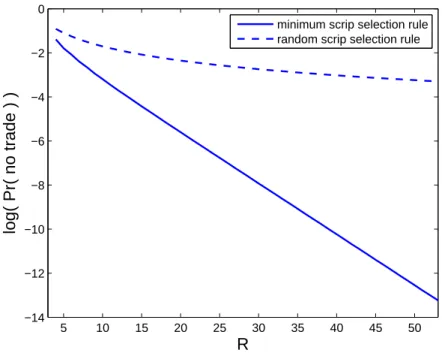
In particular, the solid curve in Figure 2-1 illustrates that the probability that trade does not occur, due to lack of scrips by the service requester, appears log linearly decreasing with the number of scrips 𝑅 in the system when 𝑅 is sufficiently large; each point on this curve is obtained through standard numerical iteration approaches to compute steady state probabilities for a 3 player Markov Chain. In comparison, the dotted curve represents the same probability following the random provider selection rule. It is clear that the chance of no trade is much lower with the minimum scrip selection rule than the random provider selection rule. More generally, we are able to obtain a closed form expression of the probability of no trade following the random provider selection rule (see Proposition 7 in the Appendix, and [Kash et al., 2012a] Lemmas A.3 and A.4 for steady state probabilities in more general settings).

(25)

5 10 15 20 25 30 35 40 45 50 −14 −12 −10 −8 −6 −4 −2 0 R log( Pr( no trade ) )

minimum scrip selection rule random scrip selection rule

Figure 2-1: Probability of no trade with 𝑁 = 3 players.

2.3 Stochastic Game and Optimality of Minimum Scrip

Selection Rule

In this section, we remove the existence of a central planner, and we formally define the game in which the pair of players selected to be potential trade partners can decide whether to exchange a scrip for service. We then demonstrate that even in the absence of a central planner, the minimum scrip selection rule, ¯𝜋, achieves the maximum social welfare obtained in the central planner setting under certain conditions, which corresponds to the Folk The-orem for stochastic games (see, e.g., [Fudenberg and Tirole, 1991]). Furthermore, we show that in the game setting there exist thresholds on the discount factor as well as the relative benefit of receiving a service above which all players have the incentive to trade a scrip for service whenever the service requester has at least one scrip.

(26)

2.3.1 Stochastic Game

Now we consider a game in which all players follow a particular service provider selection policy 𝜋 ∈ Π; we assume that no players collude. We focus on a stochastic game setting where the planning horizon is infinite, due to the well known distinction between finite horizon stochastic games and infinite horizon stochastic games (see, e.g., [Fudenberg and Tirole, 1991]). In our setting, if the planning horizon was finite, given that scrips have no salvage value at the end of the horizon, no type 0 player would offer service and suffer a negative utility −𝑐 in the last period. Using backward induction and following the same logic throughout the time horizon, no trade ever occurs in any finite horizon game.

In the infinite horizon setting, each player’s strategy may depend on the entire history of the game. In particular, we denote vector 𝜃 = (𝑟, 𝑗, 𝑖, Ω) to represent the “state of game” at each period, in which 𝑟 is the scrip distribution vector, 𝑗 is the service requester, 𝑖 is the player selected to be the service provider according to selection rule 𝜋(𝑟, 𝑗), and set Ω contains all players who 𝑖) have never refused to trade a scrip for service with anyone within set Ω, and 𝑖𝑖) have never traded with anyone not in set Ω at the time of trade1_{. Obviously, in}

the beginning of the time horizon, Ω contains all the 𝑁 players in the game. Further denote set 𝐷𝑘(𝜃)to represent player 𝑘 ∈ 𝑁’s action space at state of game 𝜃. In particular, if player

𝑗 has positive scrips (𝑟𝑗 > 0), she can choose whether or not to give one scrip to player 𝑖

in exchange for service (𝑑𝑗 = 1), or not to spend the scrip for service (𝑑𝑗 = 0); therefore,

𝐷𝑗(𝑟, 𝑗, 𝑖, Ω) = {1, 0}. Player 𝑖, on the other hand, can choose whether to accept the scrip

and serve player 𝑗 (𝑑𝑖 = 1) or not (𝑑𝑖 = 0); therefore, 𝐷𝑖(𝑟, 𝑗, 𝑖, Ω) = {1, 0}. Any player other

than 𝑖 and 𝑗 must take no action, so 𝐷𝑘(𝑟, 𝑗, 𝑖, Ω) = {0} for 𝑘 ̸= 𝑖, 𝑗. Note that at state of

game 𝜃 = (𝑟, 𝑗, 𝑖, Ω), trade of a scrip for service occurs only if 𝑟𝑗𝑑𝑖𝑑𝑗 > 0. Denote the action

profile 𝐷(𝜃) = ×𝑘∈𝑁𝐷𝑘(𝜃), with element 𝑑(𝜃) = (𝑑𝑘(𝜃))𝑘∈𝑁 ∈ 𝐷(𝜃).

Given state of game 𝜃 = (𝑟, 𝑗, 𝑖, Ω) and action profile 𝑑, single period utilities for players 𝑖 and 𝑗 depend on whether or not trade occurred; 𝑢𝑖(𝜃, 𝑑) = −𝑐 and 𝑢𝑗(𝜃, 𝑑) = 𝑢if 𝑟𝑗𝑑𝑖𝑑𝑗 > 0

(trade occurred), and 𝑢𝑖(𝜃, 𝑑) = 𝑢𝑗(𝜃, 𝑑) = 0 if 𝑟𝑗𝑑𝑖𝑑𝑗 = 0 (trade did not occur). In either

1_{In the stochastic game, generally speaking, the service provider selection rule may allow selection of}

another player in case a first selected player rejects to serve. Such a generalized selection rule 𝜋 maps the distribution of scrips to a sequence of provider selections, contingent upon acceptance. All equilibrium results hold with this generalization.

(27)

case, for any player 𝑘 ̸= 𝑖, 𝑗, the utility 𝑢𝑘(𝜃, 𝑑) = 0. Given service provider selection rule

𝜋, each player tries to maximize her own total utility over an infinite horizon with discount factor 𝛾 ∈ (0, 1).

Following [Myerson, 1997], it is sufficient to consider stationary strategy profiles, i.e., strategies that only depend on state of the game rather than the entire history. Specifically, consider stationary strategy 𝜏𝑘 for player 𝑘 that maps state of the game 𝜃 to a particular

action 𝑑𝑘 ∈ 𝐷𝑘(𝜃) and the corresponding policy profile for all players, denoted as 𝜏 = (𝜏𝑘).

Let 𝑣𝑘(𝜏, 𝜃) denote player 𝑘’s expected 𝛾-discounted average payoff if players commit to

stationary policy profile 𝜏 and the current state of game is 𝜃. Further denote 𝑌𝑘(𝜏, 𝑑𝑘, 𝑣𝑘, 𝜃)

to represent player 𝑘’s discounted average payoff starting from state 𝜃 if all players commit to stationary policy 𝜏 except player 𝑘, who deviates in the first round with action 𝑑𝑘,

𝑌𝑘(𝜏, 𝑑𝑘, 𝑣𝑘, 𝜃) = (1 − 𝛾)𝑢𝑘(︀𝜃, (𝑑𝑘, 𝜏−𝑘(𝜃)))︀ + 𝛾 𝑁 ∑︁ 𝑗′_∈𝑁 𝑣𝑘 (︁ 𝜏,(︀𝑟′, 𝑗′, 𝜋(𝑟′, 𝑗′), 𝜔(𝜃, 𝑑𝑘) )︀)︁ , where 𝜔(𝜃, 𝑑𝑘) = Ω if 𝑑𝑘= 1 or 𝑘 ̸= 𝑖, 𝑗 , and 𝜔(𝜃, 𝑑𝑘) = Ω ∖ 𝑘 if 𝑑𝑘 = 0 and 𝑘 = 𝑖 or 𝑗 .

Theorem 7.1 of [Myerson, 1997] states that the stationary strategy 𝜏 is an equilibrium strategy profile of the stochastic game if for every player 𝑘 we have

𝑣𝑘(𝜏, 𝜃) = max 𝑑𝑘∈𝐷𝑘(𝜃)

𝑌𝑘(𝜏, 𝑑𝑘, 𝑣𝑘, 𝜃) . (2.9)

In other words, if each player’s optimal strategy is to not deviate from 𝜏 in a single period, then 𝜏 is an equilibrium strategy profile. Using these notations, it is straightforward to verify the following result, which we will use to prove Lemma 3 to support the Folk Theorem result. Lemma 1. Following any service provider selection rule 𝜋 ∈ Π, it is an equilibrium for every player 𝑖 = 𝜋(𝑟, 𝑗) to always refuse providing service. The corresponding equilibrium discounted average payoff for each player is 0.

In order to demonstrate the next result, we define the always trade strategy profile ¯𝜏 to be such that in each time period the service requester always chooses to pay for service

(28)

whenever she has positive scrips, and the selected type 0 player always chooses to provide service as long as the service requester belongs to set Ω and refuses to provide service if the service requester does not belong to set Ω. We also define unichain selection rules to be the set of service provider selection rules under which if players follow the always trade strategy profile, the resulting Markov chain on the state space 𝑆 has a single recurrent class. It is easy to verify that both the minimum and random provider selection rules mentioned earlier in the chapter are examples of unichain selection rules, along with many others.

Lemma 2. Following any unichain service provider selection rule 𝜋, if players follow the always trade strategy ¯𝜏, the total discounted payoff is positive for all players at any state 𝑠 for 𝛾 close enough to 1.

Proof: Since policy 𝜋 is unichain, the long run average payoff is independent of the initial state (𝑟, 𝑗) ( [Bertsekas, 2007]). In any time period, the chance that a random service requester has a positive number of scrips is at least 1/𝑁. As a result, by following the always trade strategy profile, the expected social welfare gain per time period is at least (𝑢 − 𝑐)/𝑁, which lower bounds the long run average social welfare gain. Since the 𝑁 players are indistinguishable, the per player long run average payoff is lower bounded by (𝑢−𝑐)/𝑁2 _>

0.

Following Proposition 4.1.2 of [Bertsekas, 2007], the total average discounted payoff 𝑣𝑘(¯𝜏 , 𝜃) converges to the long run average payoff as discount 𝛾 approaches 1, and

there-fore is also positive.

Lemma 2 essentially states that when the discount factor is close enough to 1, the value function is positive at all states under any unichain service provider selection rule and the always trade strategy. Following the idea behind the Folk Theorem, if a player wants to refuse requesting or providing service in exchange for a scrip, and therefore deviate from the always trade strategy, the entire group of players can punish this player by refusing to provide service in the future. This results in an inferior, zero, total future utility for the focal player. This threat prevents a player from deviating from the always trade strategy. The following result summarizes this idea.

(29)

Lemma 3. Under any unichain service provider selection rule 𝜋, there exists a 𝛾 such that for any 𝛾 ∈ [𝛾, 1], the always trade strategy profile ¯𝜏 is an equilibrium.

This result follows from the Folk Theorem for stochastic games (Theorem 9, [Dutta, 1995]). The complete proof in the Appendix verifies the conditions of Theorem 9 in [Dutta, 1995] based on Lemmas 1 and 2.

Lemma 3 implies that as the discount factor is getting close to 1, the centralized optimal solution can be achieved in the stochastic game. This is by no means surprising, in light of the Folk Theorem. The above sequence of lemmas, however, motivates our next analysis of the always trade strategy when either the policy 𝜋 is not unichain or the discount factor is not sufficiently close to 1.2

2.3.2 Always Trade Strategy

In this section we show that under certain conditions the central planner’s optimal social welfare obtained in Section 2.2.1 can be achieved in the stochastic game. Motivated by Lemmas 1 - 3, we next focus on the case in which each player follows the always trade strategy.

Without loss of generality, denote 𝑉 (𝑠) to represent the total discounted value function of player 1 at state of the system 𝑠 = (𝑟, 𝑗), under service provider selection rule 𝜋 and the always trade strategy ¯𝜏. Therefore, function 𝑉 satisfies the following recursive equation,

𝑉 = 𝑇 𝑉 , (2.10) in which (𝑇 𝑉 )(𝑟, 1) = ⎧ ⎨ ⎩ (𝛾/𝑁 )∑︀ 𝑗′𝑉 (𝑟, 𝑗′) , 𝑟1 = 0 𝑢 + 𝛾/(𝑁 |Υ𝜋(𝑟, 1)|)∑︀ 𝑗′ ∑︀ 𝑖∈ϒ𝜋_(𝑟,1)𝑉 (𝑟 − 𝑒1+ 𝑒𝑖, 𝑗′) , 𝑟1 > 0 , (2.11)

2_{When the policy 𝜋 is not unichain, Lemma 2 does not hold. Therefore Condition 1 of Dutta’s theorem}

may be violated. Furthermore, Dutta’s Folk Theorem for stochastic games requires the discount factor to be sufficiently close to 1.

(30)

and (𝑇 𝑉 )(𝑟, 𝑗) = ⎧ ⎪ ⎪ ⎪ ⎨ ⎪ ⎪ ⎪ ⎩ (𝛾/𝑁 )∑︀ 𝑗′𝑉 (𝑟, 𝑗′) , 𝑟𝑗 = 0 𝛾/(𝑁 |Υ𝜋_{(𝑟, 𝑗)|)}∑︀ 𝑗′ ∑︀ 𝑖∈ϒ𝜋_(𝑟,𝑗)𝑉 (𝑟 − 𝑒𝑗 + 𝑒𝑖, 𝑗′) , 𝑟𝑗 > 0, 1 ̸∈ Υ𝜋(𝑟, 𝑗) (︁ −𝑐 + 𝛾/𝑁∑︀ 𝑗′ ∑︀ 𝑖∈ϒ𝜋_(𝑟,𝑗)𝑉 (𝑟 − 𝑒𝑗+ 𝑒𝑖, 𝑗′) )︁ /|Υ𝜋(𝑟, 𝑗)| , 𝑟𝑗 > 0, 1 ∈ Υ𝜋(𝑟, 𝑗) . (2.12) Here the set Υ𝜋_{(𝑟, 𝑗)}_{represents the set of players eligible to be selected as the service provider,}

according to selection policy 𝜋; we assume ties are broken randomly. For example, under the minimum scrip selection rule ¯𝜋, set Υ𝜋¯_{(𝑟, 1)} _{includes all players who hold the smallest}

number of scrips, excluding player 1. If the cardinality of the set |Υ𝜋_{(𝑟, 𝑗)| > 1}_{, each player}

in the set has the same chance of being chosen to be the service provider. When the service provider selection rule is clear in the context, we remove the superscript in Υ𝜋 _{for simplicity.}

Using the recursive expression of value function 𝑉 , we show the following result.

Proposition 2. For any given service provider selection rule 𝜋 ∈ Π and model parameters 𝑢, 𝑐, 𝑁 and 𝑅, there is a unique threshold ¯𝛾 ∈ (0, 1), such that 𝑉 (𝑟, 𝑗) ≥ 0 for all 𝑟 and 𝑗 if and only if 𝛾 ≥ ¯𝛾.

Proof: Denote 𝑉𝛾 to be the solution to recursive equations (2.10)-(2.12). That is,

𝑉𝛾 _{= 𝑇 𝑉}𝛾_{. Now consider a slightly revised value iteration,}

(𝑇𝛾𝑉 )(𝑟, 1) = ⎧ ⎨ ⎩ (𝛾/𝑁 )∑︀ 𝑗′𝑉 (𝑟, 𝑗′) , 𝑟1 = 0 𝛾𝑢 + 𝛾/(𝑁 |Υ(𝑟, 1)|)∑︀ 𝑗′ ∑︀ 𝑖∈ϒ(𝑟,1)𝑉 (𝑟 − 𝑒1+ 𝑒𝑖, 𝑗 ′_{) , 𝑟} 1 > 0 , (𝑇𝛾𝑉 )(𝑟, 𝑗) = ⎧ ⎪ ⎪ ⎪ ⎨ ⎪ ⎪ ⎪ ⎩ (𝛾/𝑁 )∑︀ 𝑗′𝑉 (𝑟, 𝑗′) , 𝑟𝑗 = 0 𝛾/(𝑁 |Υ(𝑟, 𝑗)|)∑︀ 𝑗′ ∑︀ 𝑖∈ϒ(𝑟,𝑗)𝑉 (𝑟 − 𝑒𝑗 + 𝑒𝑖, 𝑗′) , 𝑟𝑗 > 0, 1 ̸∈ Υ(𝑟, 𝑗) (︁ −𝛾𝑐 + 𝛾/𝑁 ∑︀ 𝑗′ ∑︀ 𝑖∈ϒ(𝑟,𝑗)𝑉 (𝑟 − 𝑒𝑗 + 𝑒𝑖, 𝑗 ′₎)︁_{/|Υ(𝑟, 𝑗)| , 𝑟} 𝑗 > 0, 1 ∈ Υ(𝑟, 𝑗) .

Denote ˆ𝑉𝛾 _{to be the solution to ˆ𝑉}𝛾 _{= 𝑇}𝛾_𝑉_ˆ𝛾_{, which is also the total discounted value function}

of player 1 with 𝛾𝑢 and 𝛾𝑐 as the benefit and cost of trade instead of 𝑢 and 𝑐. Therefore, ˆ

𝑉𝛾 _{= 𝛾𝑉}𝛾_.

Now consider a discount factor ˆ𝛾 such that 𝑉^𝛾 _{≥ 0}, which implies ˆ𝑉𝛾^ _{≥ 0}. Consider

any discount factor 𝛾′ _{such that 𝛾}′ _{> ˆ}_𝛾_{. We have 𝑇}𝛾′_ˆ

(31)

convergence of the value iteration algorithm and monotonicity of the operator 𝑇𝛾 _(Corollary

1.2.1.1 and Lemma 1.1.1 in [Bertsekas, 2007]), ˆ 𝑉𝛾′ = lim 𝑡→∞(𝑇 𝛾′₎𝑡_𝑉_ˆ𝛾^ _{≥ lim} 𝑡→∞(𝑇 ^ 𝛾₎𝑡_𝑉_ˆ𝛾^ _{= ˆ}_𝑉^𝛾 _{≥ 0 ,} which implies 𝑉𝛾′ = ˆ𝑉𝛾′/𝛾′ ≥ 0.

Note that this result is stronger than Lemma 2 because it holds for policies 𝜋 that are not unichain and shows a unique threshold ¯𝛾. Parallel to Proposition 2, we have the following intuitive result.

Proposition 3. For any given service provider selection rule 𝜋 ∈ Π and model parameters 𝛾, 𝑁 and 𝑅, there is a unique threshold on 𝑢/𝑐, such that 𝑉 (𝑟, 𝑗) ≥ 0 for all 𝑟 and 𝑗 if and only if 𝑢/𝑐 is larger than this threshold.

The proof is very similar to the proof of Proposition 2 and thus is omitted here.

Propositions 1, 2 and 3 imply the following main result of this section, which is stronger than Lemma 3.

Theorem 2. For any model parameters 𝑢, 𝑐, 𝑁 and 𝑅, there is a unique threshold of the discount factor, ¯𝛾, such that when 𝛾 > ¯𝛾, the centralized optimal social welfare is achieved in equilibrium. That is, under the minimum scrip selection rule ¯𝜋, in equilibrium all players follow the always trade strategy.

Similarly, for any given model parameters 𝛾, 𝑁 and 𝑅, there is a unique threshold on 𝑢/𝑐, above which the centralized optimal social welfare is achieved in equilibrium by all players following the always trade strategy under the minimum scrip selection rule.

The equilibrium result is proved by applying the definition of the always trade strategy to equilibrium condition (2.9).

2.4 Number of Scrips in the System

In the previous section we demonstrated the optimality of the minimum scrip selection rule in the stochastic game setting with a fixed number of scrips and when the discount factor

(32)

is large enough. In this section we investigate the appropriate number of scrips to ensure that always trade is an equilibrium strategy under the minimum scrip selection rule. In particular, we show that under fairly general conditions, there is a unique threshold of the number of scrips in the system, below which always trade is an equilibrium. Furthermore, the threshold increases with the discount factor 𝛾 and the benefit of receiving service, 𝑢/𝑐.

First we present a condition under which no matter how many scrips are in the system, the value function for any state is non-negative, implying that always trade is an equilibrium. Theorem 3. Under any service provider selection rule 𝜋 ∈ Π, if

𝑢 𝑐 ≥

𝑁

𝛾 , (2.13)

no matter how many scrips are in the system, the value function 𝑉 that solves the recursive equations (2.10)-(2.12) is non-negative; that is, the always trade strategy is an equilibrium. The proof is presented in the Appendix.

The condition (2.13), rewritten as 𝑐 ≤ 𝛾𝑢/𝑁, reflects the trade-off between the cost of serving today versus the expected benefit of receiving service tomorrow. It is intuitive that if the cost of earning a scrip today is less than the expected benefit of spending it in the next period, providing service never generates a negative net expected profit. Interestingly, the condition does not depend on the service provider selection rule.

Since the condition is rather restrictive, we next analyze what happens under the min-imum scrip selection rule when the condition 𝑐 ≤ 𝛾𝑢/𝑁 is violated. First, we present a technical characterization of recurrent states, which is somewhat interesting in its own right and useful for proving our main result.

Lemma 4. Consider the case when 𝑅 ≥ 𝑁, i.e., the number of scrips in the system is no less than the number of players. Under the minimum scrip selection rule and always trade strategy, any state with more than one player having 0 scrips is transient.

The proof is based on induction on the number of players with 0 scrips. The detailed proof is presented in the Appendix. Lemma 4 allows us to restrict attention to only those

(33)

states where no more than 1 player has 0 scrips, which will be useful to prove Proposition 4, constituting the foundation of our main result, Theorem 4.

Analogous to the symmetry condition (C1) in the central planner setting, Lemma 5 below provides a symmetry argument needed for the proofs of Propositions 4 and 5.

Lemma 5. Assume value function 𝑉 satisfies recursive equations (2.10)-(2.12) for a system with 𝑅 ≥ 𝑁 scrips with the minimum scrip selection rule. For any nonnegative integer vectors 𝑟 and 𝑟′ _{such that ∑︀}

𝑗𝑟𝑗 = 𝑅 and ∑︀𝑗𝑟 ′

𝑗 = 𝑅 with 𝑟𝑘 = 𝑟′𝑘 for all 𝑘 except 𝑙 ̸= 1,

𝑚 ̸= 1, where 𝑟𝑙 = 𝑟𝑚′ and 𝑟𝑚 = 𝑟′𝑙, ∑︁ 𝑗 𝑉 (𝑟, 𝑗) =∑︁ 𝑗 𝑉 (𝑟′, 𝑗) . (2.14)

The proof is presented in the Appendix.

Proposition 4. Assume value function 𝑉 satisfies recursive equations (2.10)-(2.12) for a system with 𝑅 ≥ 𝑁 scrips with the minimum scrip selection rule, and value function ¯𝑉 satisfies recursive equations (2.10)-(2.12) for a system with the same parameters except with 𝑅 + 1 scrips. Further, assume that

𝑢 𝑐 ≤ 𝑁 𝛾 [︂ 𝑁 𝛾 − (𝑁 − 1) ]︂ − (𝑁 − 1) . (2.15)

For any nonnegative integer vector 𝑟 in the recurrent class such that ∑︀𝑗𝑟𝑗 = 𝑅, and any

player index 𝑗 and 𝑘 ̸= 1, we have ¯ 𝑉 (𝑟 + 𝑒𝑘, 𝑗) ≤ 𝑉 (𝑟, 𝑗) , (2.16) ∑︁ 𝑗 ¯ 𝑉 (𝑟 + 𝑒1, 𝑗) − ∑︁ 𝑗 𝑉 (𝑟, 𝑗) ≤ 𝑐𝑁 𝛾 , ∀𝑟 : 𝑟1 > 0 , and (2.17) ∑︁ 𝑗 ¯ 𝑉 (𝑟 + 𝑒1, 𝑗) − ∑︁ 𝑗 𝑉 (𝑟, 𝑗) ≤ 𝑁 𝛾 [︂ 𝑁 𝛾 − (𝑁 − 1) ]︂ 𝑐 , ∀𝑟 : 𝑟1 = 0 . (2.18)

Property (2.16) is a monotonicity property for value functions across different state spaces, and it states that if we inject one more scrip in the system, every player, other than the one who receives the scrip, is worse off (measured by the value function). The basic

(34)

intuition behind it is that giving more scrips to others makes a player more likely to become the minimum scrip holder, and therefore work sooner than otherwise. For the one who does receive the additional scrip, while it is intuitive that the person is better off, properties (2.17) and (2.18) show that the benefit is, in fact, upper bounded. The intuition is that even though the player who receives the additional scrip is better off by, at some point, spending it for service, such a trade is followed by a state where the additional scrip belongs to someone else, therefore the player will be worse off afterwards, following (2.16). The basic logic of the proof for Proposition 4 is that these properties are preserved through value iteration. The complete proof, however, needs to verify the properties under all possible scenarios of scrip distribution among players in both the 𝑅 scrip system as well as the 𝑅 + 1 scrip system. Furthermore, in order to establish each one of properties (2.16)-(2.18), we need all the prop-erties to hold to begin the value iteration, as well as condition (2.15). As a result, the proof is rather involved and is presented in the Appendix.

Property (2.16) is the key property that we focus on. It implies that there is a threshold (possibly infinity) on the number of scrips, above which the value function at some state may become negative. When the value function does become negative, the threat of zero utility does not work anymore, and the corresponding player at this state is better off claiming bankruptcy by leaving the group. In order to prevent such an undesirable outcome, the number of scrips issued in the system must be lower than this threshold. As discussed in Section 2.2.1, the social welfare of the system increases with the number of scrips. Therefore, assuming players follow the minimum scrip selection rule, the system designer will choose the number of scrips in the system to be just below this threshold in order to achieve the greatest possible social welfare while making it in each player’s best interest to not leave the group.

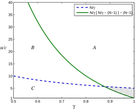
The monotonicity property (2.16), however, holds only under condition (2.15). Figure 2-2 depicts the condition. That is, in the area below the solid curve, due to monotonicity there is a threshold on the number of scrips (possibly infinity), below which always trade is an equilibrium strategy. The dashed curve in Figure 2-2 corresponds to condition (2.13) in Theorem 3. In the area above the dashed curve, no matter how many scrips are in the system, always trade is an equilibrium strategy. These curves partition Figure 2-2 into four

(35)

0.5 0.6 0.7 0.8 0.9 1 1 5 10 15 20 25 30 35 40 γ A C B u/c N/γ N/γ [ N/γ − (N−1) ] − (N−1)

Figure 2-2: Conditions (2.13) and (2.15), with 𝑁 = 5.

ares. In area A, no matter how many scrips are in the system, always trade is an equilibrium strategy. In area B, adding a scrip to the system decreases every player’s total discounted value except that of the player with the additional scrip; however, we know that each player’s total discounted value remains positive and thus no matter how many scrips are in the system, always trade is an equilibrium. In area C, adding a scrip to the system decreases every player’s total discounted value except that of the player with the additional scrip; in this case, there is a threshold (possibly infinity) on the number of scrips above which at least one of the player’s total discounted value is negative. This leaves the shaded area depicted in the figure not covered by theoretical results. Later in Section 2.4.1, we conduct a numerical study on the shaded area, which indicates that although the monotonicity property (2.16) does not hold, it is very likely that there still exists a unique upper bound on the number of scrips.

Theorem 2 in the previous section states that for any given number of scrips 𝑅, there is a threshold on 𝛾 above which the value function 𝑉 is always positive. Proposition 4 further states that under condition (2.15), for a given discount 𝛾, there is a threshold 𝑅 below which the value function 𝑉 is always positive. The combination of the two results implies that

(36)

in the 𝑅 − 𝛾 space, the region that guarantees that value function 𝑉 is always positive is characterized by a threshold in 𝑅 that is monotone in 𝛾. The result is formally stated in the following Theorem. (The result on 𝑢/𝑐 follows the exact same argument.)

Theorem 4. In a scrip system with 𝑁 players and at least 𝑁 scrips, for any given set of model parameters such that

𝑢 𝑐 ≥ 2(𝑁 − 1) √ 𝑁2_{+ 4𝑁 − 4 − 𝑁} , or 𝛾 ≤ 𝑁 (√𝑁2_{+ 4𝑁 − 4 − 𝑁 )} 2(𝑁 − 1) , (2.19)

there is an upper bound ¯𝑅 (possibly infinity) on the number of scrips, below which always trade is an equilibrium strategy under the minimum scrip selection rule, and the system optimal social welfare is achieved in the game. Furthermore, the upper threshold ¯𝑅 increases with 𝛾 and 𝑢/𝑐.

Sufficient condition (2.19) is obtained by equating conditions (2.13) and (2.15). Illus-trated in Figure 2-2, condition (2.19) covers the area to the left and above of the intersection between the solid and dashed curves. As we will demonstrate in numerical studies in Section 2.4.1, the monotone threshold structure presented in Theorem 4 likely holds even without these conditions being met.

2.4.1 Shaded Area

We do not have theoretical results when conditions (2.13) and (2.15) are both violated, de-picted by the shaded area in Figure 2-2. Therefore, we conducted numerical studies to check the structure of the value function in its minimum recurrent state. In particular, we take a grid of values for 𝑢/𝑐 and 𝛾 in the shaded area when 𝑁 = 3,3 _{and we see how the minimum}

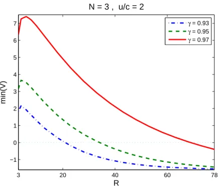
value function’s value (over recurrent states) changes with increasing 𝑅. We observe that in every case, the value function is unimodal and therefore monotonically decreases as 𝑅 increases to be large enough. Figure 2-3 depicts one such example.

The findings indicate that when condition (2.15) in Proposition 4 is violated, a player’s value function does not always decrease monotonically with more scrips given to others. On 3_{Since the state space grows exponentially with 𝑁, which poses significant computational challenges, we}

(37)

3 20 40 60 78 −1 0 1 2 3 4 5 6 7 R min(V) N = 3 , u/c = 2 γ = 0.93 γ = 0.95 γ = 0.97

Figure 2-3: The non-monotone, unimodal structure of the value function in its minimum recurrent state.

the other hand, in our numerical examples, it always first increases when the number of scrips 𝑅 is small, and then decreases. Therefore, as long as the minimum value function over recurrent states is positive at the smallest scrip number 𝑅 = 𝑁, there still is a unique upper bound (possibly infinity) on the number of scrips, below which the value function is positive in all states. If so, the threshold on the number of scrips in the system increases with 𝛾 and 𝑢/𝑐, even without the necessity of condition (2.19).

The following result indicates that when 𝑅 = 𝑁 the value function is indeed positive in all recurrent states.

Proposition 5. Assume 𝑅 = 𝑁 and 𝑢 𝑐 ≥ 𝑁 𝛾 [︂ 𝑁 𝛾 − (𝑁 − 1) ]︂ − (𝑁 − 1) . (2.20)

The value function 𝑉 that solves the recursive equations (2.10)-(2.12) under the minimum scrip selection rule is positive in all recurrent states.

(38)

2.4.2 Generalizations

In this section, we describe two generalizations of our model. The first relates our model to the random provider selection rule proposed in previous literature. The second adapts our model for potential use in kidney exchange networks.

Random Provider Selection Rule

It is important to note that there is a possibility that a different service provider selection rule may permit a greater number of scrips than the minimum scrip selection rule. We have shown that for a given number of scrips in the system, the minimum scrip selection rule achieves the maximum social welfare. It could be possible, however, that a different service provider selection rule outperforms the minimum scrip selection rule because it allows more scrips in the system without a player defaulting compared to the minimum scrip selection rule. Here we analyze the random provider selection rule, a common selection rule considered in previous literature. More precisely, we consider a generalization of the minimum scrip selection rule that also includes the random provider selection rule.

In particular, consider the following service provider selection rule. First, 𝐾 players out of the 𝑁 −1 players are randomly selected as “potential providers”. Then the potential provider who has the least number of scrips is selected as the service provider. Such a setting covers the possibility that not every player can provide service in each period, which, to a certain extent, relates to settings studied in [Kash et al., 2007], [Kash et al., 2012a], and [Kash et al., 2012b]. Obviously, when 𝐾 = 1, we have the random provider selection rule, while the case 𝐾 = 𝑁 − 1 is the minimum scrip selection rule. The recursive equations (2.10)-(2.12) are customized to 𝑉 = 𝑇 𝑉 , where

(𝑇 𝑉 )(𝑟, 𝑗) = E𝜅𝑗[(Ξ𝜅𝑗𝑉 )(𝑟, 𝑗)] , (2.21)

(39)

players who are not 𝑗, and Ξ𝜅𝑗𝑉 follows (Ξ𝜅1𝑉 )(𝑟, 1) = ⎧ ⎨ ⎩ (𝛾/𝑁 )∑︀ 𝑗′𝑉 (𝑟, 𝑗′) , 𝑟₁ = 0 𝑢 + 𝛾/(𝑁 |Υ𝜅1(𝑟, 1)|) ∑︀ 𝑗′ ∑︀ 𝑖∈ϒ_𝜅1(𝑟,1)𝑉 (𝑟 − 𝑒1+ 𝑒𝑖, 𝑗 ′_{) , 𝑟} 1 > 0 , (2.22) and (Ξ𝜅𝑗𝑉 )(𝑟, 𝑗) = ⎧ ⎪ ⎪ ⎪ ⎨ ⎪ ⎪ ⎪ ⎩ (𝛾/𝑁 )∑︀ 𝑗′𝑉 (𝑟, 𝑗′) , 𝑟𝑗 = 0 𝛾/(𝑁 |Υ𝜅𝑗(𝑟, 𝑗)|) ∑︀ 𝑗′ ∑︀ 𝑖∈ϒ_𝜅𝑗(𝑟,𝑗)𝑉 (𝑟 − 𝑒𝑗+ 𝑒𝑖, 𝑗 ′_{) ,} _𝑟 𝑗 > 0, 1 ̸∈ Υ𝜅𝑗(𝑟, 𝑗) (︁ −𝑐 + 𝛾/𝑁∑︀ 𝑗′ ∑︀ 𝑖∈ϒ_𝜅𝑗(𝑟,𝑗)𝑉 (𝑟 − 𝑒𝑗 + 𝑒𝑖, 𝑗 ′₎)︁_/|Υ 𝜅𝑗(𝑟, 𝑗)| , 𝑟𝑗 > 0, 1 ∈ Υ𝜅𝑗(𝑟, 𝑗) . (2.23) Here Υ𝜅𝑗(𝑟, 𝑗) represents the set of minimum scrip holders among players in the set 𝜅𝑗.

Similar to Proposition 4 for the minimum scrip selection rule, the following result holds for the general service provider selection rule described above, including the random provider selection rule.

Proposition 6. Assume value function 𝑉 satisfies 𝑉 = 𝑇 𝑉 , where operator 𝑇 is defined in equations (2.21)-(2.23), and value function ¯𝑉 satisfies the same recursive equation in a system with the same parameters except with 𝑅 + 1 scrips. Further, assume that

𝑢 𝑐 ≤

𝑁

𝛾 − (𝑁 − 1) . (2.24)

For any nonnegative integer vector 𝑟 such that ∑︀𝑗𝑟𝑗 = 𝑅 and any player index 𝑗 and 𝑘 ̸= 1,

we have ¯ 𝑉 (𝑟 + 𝑒𝑘, 𝑗) ≤ 𝑉 (𝑟, 𝑗) , and (2.25) ∑︁ 𝑗 ¯ 𝑉 (𝑟 + 𝑒1, 𝑗) − ∑︁ 𝑗 𝑉 (𝑟, 𝑗) ≤ 𝑐𝑁 𝛾 . (2.26)

The proof is similar to that of Proposition 4 and is presented in the Appendix.

For similar reasons as discussed above for the minimum scrip selection rule, property (2.25) implies that there is a threshold (possibly infinity) on the number of scrips in the system, above which the value function at some state may become negative. Numerical studies similar to those described in Section 2.4.1 suggest that conditions (2.13) and (2.24)

(40)

are sufficient, but not necessary, for the threshold structure to hold.

Interestingly, therefore, both the minimum scrip selection rule and the random provider selection rule permit a threshold number of scrips in the system (possibly infinity), above which the system crashes. Depending upon the system parameters 𝑢, 𝑐, 𝑁, and 𝛾, numerical results show that sometimes the minimum scrip selection rule permits at least as many scrips as the random provider selection rule; in this case, the minimum scrip selection rule is the preferable service provider selection rule for the scrip system because it provides a greater social welfare. For other parameters, though, the random provider selection rule permits more scrips than the minimum scrip selection rule, and in some cases the difference is enough to cause the random provider selection rule to outperform the minimum scrip selection rule in terms of social welfare. Depending on the system parameters and application, the system designer may choose to compare the performance of the minimum scrip selection rule and the random provider selection rule before creating the scrip system. Since both exhibit a threshold property on the number of permissable scrips in the system, this should be relatively simple to do.

Adaptation for Kidney Exchange Networks

Over 90,000 patients are in need of a kidney transplant in the United States ( [Ashlagi and Roth, 2012]). Several of these patients have a living donor (typically a family member or close friend) who is willing to give them one of their kidneys to save the patient’s life; we will call this couple a "patient-donor pair". The donor’s blood and tissue types must be compatible with the patient’s in order for the kidney transplant to be successful. Since this is often not the case, "kidney exchange networks" have been set up around the country to help match patient-donor pairs with other patient-donor pairs such that the donor of one pair can give his or her kidney to the patient of the other pair and vice versa4_.

Since these exchanges are usually simultaneous and in the same location, these kidney exchange networks are typically regional and consist of member hospitals in that region. 4_{In some cases, patient-donor pairs are matched to form longer "chains", i.e. where the donor of pair}

A gives his kidney to the patient of pair B, the donor of pair B gives his kidney to the patient of pair C, and the donor of pair C gives his kidney to the patient of pair A. For simplicity, we will only consider an exchange/match between two pairs.