Versatile black-box optimization

(1)

Versatile Black-Box Optimization

Jialin Liu

Southern University of Science and Technology

Shenzhen, China liujl@sustech.edu.cn

Antoine Moreau

Université Clermont Auvergne, CNRS, SIGMA Clermont, Institut Pascal

Clermont-Ferrand, France antoine.moreau@univ-bpclermont.fr

Mike Preuss

LIACS, Universiteit Leiden, The Netherlands m.preuss@liacs.leidenuniv.nl

Jeremy Rapin, Baptiste Roziere

Facebook AI Research & Paris-Dauphine University

Paris, France jrapin@fb.com,broz@fb.com

Fabien Teytaud

Univ. Littoral Cote d’Opale

Calais, France teytaud@univ-littoral.fr

Olivier Teytaud

Facebook AI Research Paris, France oteytaud@fb.com

ABSTRACT

Choosing automatically the right algorithm using problem descrip-tors is a classical component of combinatorial optimization. It is also a good tool for making evolutionary algorithms fast, robust and versatile. We present Shiwa, an algorithm good at both discrete and continuous, noisy and noise-free, sequential and parallel, black-box optimization. Our algorithm is experimentally compared to competitors on YABBOB, a BBOB comparable testbed, and on some variants of it, and then validated on several real world testbeds.

CCS CONCEPTS

• Theory of computation → Optimization with randomized search heuristics.

KEYWORDS

Black-box optimization, portfolio algorithm, gradient-free algo-rithms, open source platform

ACM Reference Format:

Jialin Liu, Antoine Moreau, Mike Preuss, Jeremy Rapin, Baptiste Roziere, Fabien Teytaud, and Olivier Teytaud. 2020. Versatile Black-Box Optimization. In Genetic and Evolutionary Computation Conference (GECCO ’20), July 8–12, 2020, Cancún, Mexico. ACM, New York, NY, USA, 9 pages. https://doi.org/10. 1145/3377930.3389838

1 INTRODUCTION: ALGORITHM SELECTION

Selecting automatically the right algorithm is critical for success in combinatorial optimization: our goal is to investigate how this can be applied in derivative-free optimization. Algorithm selec-tion [8, 29, 30, 32, 48, 49] can be made a priori or dynamically. In the dynamic case, the idea is to take into account preliminary nu-merical results, i.e. starting with several optimizers concurrently and, afterwards, focusing on the best only [12, 29, 34, 35, 37, 41].

Permission to make digital or hard copies of all or part of this work for personal or classroom use is granted without fee provided that copies are not made or distributed for profit or commercial advantage and that copies bear this notice and the full citation on the first page. Copyrights for components of this work owned by others than ACM must be honored. Abstracting with credit is permitted. To copy otherwise, or republish, to post on servers or to redistribute to lists, requires prior specific permission and/or a fee. Request permissions from permissions@acm.org.

Algorithm selection among a portfolio of methods routinely wins SAT competitions. Passive algorithm selection [4] is the special case in which the algorithm selection is made a priori, from high level characteristics which are typically known in advance, such as the following problem descriptors: dimension; computational budget (measured in terms of number of fitness evaluations); degree of parallelism in the optimization; nature of variables, whether they are discrete or not, ordered or not, whether the domain is metrizable or not1; presence of constraints; noise in the objective function; and multiobjective nature of the problem. Besides the performance improvement on a given family of optimization problems, algo-rithm selection also aims at designing a versatile algoalgo-rithm, i.e. an algorithm which works for arbitrary domains and goals. We use benchmark experiments in an extendable open source platform [46], which contains a collection of benchmark problems and state of the-art gradient-free algorithms, for designing a vast algorithm se-lection process - and test it on real world objective functions. Up to our knowledge, there is no direct competitor we could compare to because algorithm selection is usually only performed on a subset of the problem types we tackle. However, we do outperform the native algorithm selection methods of Nevergrad (CMandAS and CMandAS2 [45]) on YABBOB (Fig. 2), though not by a wide margin as on testbeds far from their usual context (Fig. 3).

2 DESIGN OF SHIWA

We propose Shiwa for algorithm selection. It uses a vast collection of algorithm selection rules for optimization. Most of these rules are passive, but some are active.

2.1 Components

Our basic tools are methods from [46]:

• Continuous domains: evolution strategies (ES) [5] including the Covariance Matrix Adaptation ES [23] (abbreviated as “CMA” in this paper), estimation of distribution algorithms (EDA) [9, 38, 40], Bayesian optimization [27], particle swarm optimization (PSO) [28], differential evolution (DE) [36, 50], sequential quadratic programming [1], Cobyla [43] and Pow-ell [42].

1_{We consider that a domain is metrizable if it is equipped with a meaningful, non-binary,}

metric. In the present paper, any domain containing a discrete categorical variable is considered as non-metrizable. This is not the mathematical notion of metrizability.

(2)

• Discrete optimization: the classical (1+ 1)-evolutionary al-gorithm, Fast-GA [19] and uniform mixing of mutation rates [17]. We also include some recombination opera-tors [26].

• Noisy optimization: bandits [10], algorithms with repeated sampling [18] and population control [25].

2.2 Combinations of algorithms

Various tools exist for combining existing optimization algorithms. Terminology varies depending on authors. We adopt the follow-ing definitions: Chainfollow-ing: runnfollow-ing an algorithm, then another, and so on, initializing each algorithm using the results obtained by previous ones. In the present paper, we refer to chaining when an algorithm is run for a part of the computational budget, and another algorithm is run for the rest. For example, a memetic al-gorithm [44] running an evolution strategy at the beginning and Powell’s method [42] afterwards is a form of chaining. Passive algorithm selection [4]: the decision is made at the beginning of the optimization run, before any evaluation is performed. Active algorithm selection: preliminary results of several optimization

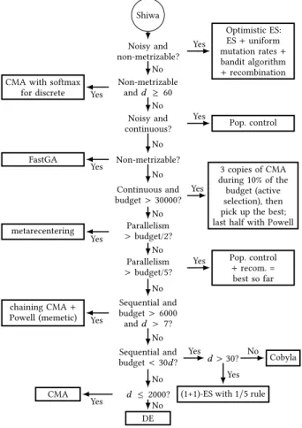
Shiwa Noisy and non-metrizable? Non-metrizable andd ≥ 60 Noisy and continuous? Non-metrizable? Continuous and budget >30000? Parallelism > budget/2? Parallelism > budget/5? Sequential and budget > 6000 andd > 7? Sequential and budget <30d ? d >30? d ≤2000? Optimistic ES: ES+ uniform mutation rates+ bandit algorithm + recombination CMA with softmax

for discrete Pop. control FastGA 3 copies of CMA during10% of the budget (active selection), then pick up the best; last half with Powell metarecentering Pop. control + recom. = best so far chaining CMA+ Powell (memetic) Cobyla

(1+1)-ES with1/5 rule CMA DE Yes No Yes No Yes No Yes No Yes No Yes No Yes No Yes No Yes No No Yes Yes _No

Figure 1: The Shiwa algorithm using the components listed in Section 2.1 based on the hypotheses presented in Section 2.4.1. The problem dimension is denoted byd.

algorithms can be used to select one of them. Splitting: the vari-ables are partitioned intok groups of variables G1, . . . , Gk. Then an

optimizerOi optimizes variables inGi; there arek optimizers

run-ning concurrently. All optimizers see the same fitness values, and, at each iteration, the candidate is obtained by concatenating the candidates proposed by each optimizer. Our optimization algorithm uses all these combinations, except splitting - though there are problems for which splitting looks like a good solution and should be used. Most of the improvement is due to passive algorithm selec-tion for moderate computaselec-tional budgets, whereas asymptotically active algorithm selection becomes critical (in particular for mul-timodal cases) and chaining (combining an evolution strategy for early stages and fast mathematical programming techniques at the end) is an important tool for large computational budget.

2.3 Preliminaries

2.3.1 Ask and tell and recommend. In the present document, we use a “ask and tell” presentation of algorithms, convenient for presenting combinations of methods. Given an optimizero, o.ask returns a candidate to be evaluated next.o.tell(x,v) informs o that the value atx is v. o.numask is the number of times o.ask has been used.o.archive is the list of visited points, with, for each of them, the list of evaluations (note that a same candidate can have been evaluated more than once, typically for noise management). o.recommend provides an approximation of the optimum; this is typically the final step of an optimization run.

2.3.2 Softmax transformations. [46] uses a softmax transforma-tion for converting a discrete optimizatransforma-tion problem into a noisy continuous optimization problem; for example, a variable with 3 possible valuesa, b and c, becomes a triplet of continuous variables va,vbandvc. The discrete variable has valuevawith probability

exp(va)/(exp(va)+ exp(vb)+ exp(vc)). Preliminary experiments

show that this simple transformation can perform well for discrete variables with more than 2 values.

2.3.3 Optimism, pessimism, progressive widening. Following [14, 24, 39, 51], we use combinations of bandits, progressive growing of the search space and evolutionary computation as already developed in Nevergrad. Such combinations are labelled “Optimistic” in Fig. 1. We refer to [46] for full details.

2.4 Algorithm design

2.4.1 Hypotheses. The design of our algorithm Shiwa relies on the following hypotheses: (i) The standard (1+ 1)-ES in continuous domains is reliable for low computational budget / high dimension. (ii) DE is a well known baseline algorithm. (iii) CMA performs well in moderate dimension [23], in particular for rotated ill-conditioned problems. (iv) Population control [25] is designed for continuous parameter optimization in high-dimension with a noisy optimiza-tion funcoptimiza-tion. (v) In other noisy optimizaoptimiza-tion settings one can use an “optimistic” combination of bandit algorithms and evolution-ary computation [24, 31] as detailed above. (vi) Population control can be used for increasing the population size in case of stagna-tion, even without noise (see the “NaiveTBPSA” code in [46]). (vii) The MetaRecentering [11] algorithm wins benchmarks in many

(3)

one-shot optimization problems in [46]: it is a combination of Ham-mersley sampling [21], scrambling [2], and automatic rescaling [11]. (vii) Continuous optimization algorithms combined with softmax can be used for discrete optimization in the case of an alphabet of cardinal > 2, according to our results in discrete settings (unpre-sented but available online2), though the case of a discrete alphabet of cardinal 2 is classically handled with classical discrete evolution-ary methods [17, 19]. (viii) Active portfolios are designed for large computational budgets (simple active portfolio methods, CMandAS and CMandAS2, are ranked as the 1st and 3rd in Figure 3a), with our proposed methods as only competitors. (ix) Some algorithms require a computational budget linear in the dimension for their ini-tialization, hence poor performance occurs when the computational budget is low compared to the dimension.

2.4.2 Algorithm: Shiwa. Based on the hypotheses presented above, we designed an algorithm structured as a decision tree (see Fig. 1). Constants in this decision tree were modified using preliminary experiments on the YABBOB testbed (defined below): Shiwa as shown in Fig. 1 is the final result. The algorithms mentioned in the boxes of Fig. 1 were preexisting in Nevergrad. Our Shiwa algorithm has been merged into Nevergrad [46] and is therefore publicly visible there3.

3 EXPERIMENTS

We compare Shiwa to algorithms from Nevergrad on a large and diverse set of problems. The results of these experiments, which have all been produced using Nevergrad, are summarized in Figs. 2, 3, 4, 5, 6 and 7. The plots are made as follows.

A limited number of rows is presented (top for the best). Each row corresponds to an optimizer. Optimizers are ranked by their scores. The score of an optimizero in a testbed T is the frequency, averaged over all problemsp ∈ T and over all optimizers o′ in-cluded in the experiments, ofo outperforming o′onp ∈ T . The problems differ in the objective function, parametrization, compu-tational budgetT , dimension d, presence of random rotation or not, and the degree of parallelization. “o outperforming o′_{on a function}

f ” means that f (o.recommend) < f (o′_{.recommend), with a truth}

value of1₂ in case of tie. Similarly to [22], the comparison is made among implementations, not among abstract algorithms; the de-tailed implementations are freely available and open sourced in [46] or in modules imported there. The columns correspond to the same optimizers, but there are more optimizers included. Still, not all optimizers are shown. Between parentheses, we can see how many cases were run out of how many instances exist; e.g. 244/252 means that there are 252 instances, but only 244 were successfully run. A failure can be due to a bug, or, in most cases, to the timeout - some optimizers become computationally expensive in high-dimensional problems and fail to complete.

Detailed setup and reproducibility. The detailed setup of our benchmarks is available online4. We did not change any setting. Our plots are those produced automatically and periodically by

2_{http://dl.fbaipublicfiles.com/nevergrad/allxps/list.html}

3_{https://github.com/facebookresearch/nevergrad/blob/master/nevergrad/}

optimization/optimizerlib.py

4_{https://github.com/facebookresearch/nevergrad/blob/master/nevergrad/}

benchmark/experiments.py

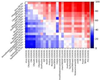
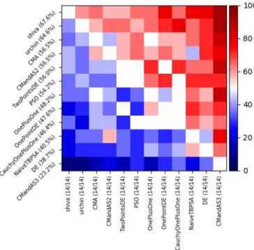
Figure 2: YABBOB: Sequential optimization with computa-tional budgetT ∈ {50, 200, 800, 3200, 12800}. Reading guide: we see that Shiwa performs better on average over all YAB-BOB experiments, than each of the other algorithms (i.e. all colors in Shiwa’s row are ≥ 50%). On average over all YAB-BOB experiments, Shiwa wins with a probability of 68.5% against other methods. “winning” means that the point rec-ommended by Shiwa had a better fitness value than the point recommended by another method (ties have truth value1₂). CMandAS and CMandAS2 are simple active portfo-lio methods present in Nevergrad and fully described there.

Nevergrad. In the artificial testbeds, Nevergrad considers cases with different numbers of critical variables (i.e. variables which have an impact on the fitness functions) and of useless variables (possibly zero). There are also rotated cases and non-rotated cases. The detailed setup is at the URL above. We provide a high-level presentation of benchmarks in the present document.

Statistical significance. Each experiment contains several set-tings. The total number of repetitions varies, but there are al-ways at least 200 random repetitions (cumulated over the dif-ferent settings) for each result displayed in our plots, and at least 5 repetitions per setting. Importantly, Nevergrad periodi-cally reruns all benchmarks with all algorithms: we can see in-dependent reruns of all results presented in the present paper at http://dl.fbaipublicfiles.com/nevergrad/allxps/list.html, plus addi-tional experiments (including a so-called YAWIDEBBOB which extends YABBOB) and results are essentially the same.

3.1 YABBOB: Yet Another Black-Box

Optimization Benchmark

YABBOB is a benchmark of black-box optimization problems. It roughly approximates BBOB [22], without exactly sticking to it. Consequently, CMA performs the best on it. YABBOB has the follow-ing advantages. It is part of a maintained and easy to use platform. Optimization algorithms are natively included in an open sourced platform. Everyone can rerun everything. There is a noisy optimiza-tion counterpart, without the issues known in BBOB [6, 7, 15, 16].

(4)

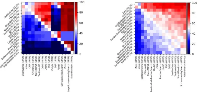
(a) YABIGBBOB: counterpart of YABBOB with T ∈ {40000, 80000}, d ∈ {2, 10, 50}. Vashi and Medusa are clones of Shiwa sometimes present in the Nevergrad platform.

(b) YAHDBBOB: counterpart of YABBOB with d ∈ {100, 1000, 3000}. CMA performs poorly in this case.

(c) YANOISYBBOB: counterpart of YABBOB with Gaussian noise added, with variance not vanishing to zero at the optimum. Shiwa is on par with methods good at noisy problems.

(d) YAPARABBOB: counterpart of YABBOB with 100 parallel workers. Medusa is a clone of Shiwa sometimes present in the Nevergrad plat-form.

Figure 3: Variants of YABBOB: YANOISYBBOB, YAHDBBOB, YAPARABBOB, YABIGBBOB, corresponding to the counterpart one with noise, the high-dimensional one, the parallel one, the big computational budget, respectively.T is the computational budget andd refers to the dimension. Shiwa is good in all categories, often performing the best, and always competing decently with the best in that category.

There are several variants, parallel or not, noisy or not, high-dimensional or not, large computational budget or not. The same platform includes a large range of real world testbeds, switching form artificial to real world is just one parameter to change in the command line.

3.2 Training: artificial testbeds

We designed Shiwa by handcrafting an algorithm as shown in Fig. 1, in which the constants have been tuned on YABBOB (Fig. 2) by trial-and-error. Then, variants of YABBOB, namely YANOISYBBOB,

YAHDBBOB, YAPARABBOB (respectively noisy, high-dimensional, and parallel counterparts of YABBOB), presented in Fig. 3, and several other benchmarks (see details in Section 3.3) are used for testing the generality of Shiwa. Tables 1 and 2 present our bench-marks. In addition, we validate our results on a wide real world testbed in Section 3.4.

(5)

(a) ARcoating: optical properties of layered structures. Shiwa is out-performed by the simple (1+ 1)-ES; for the more general Photonics problem (covering a wider range of cases) this is not the case.

(b) FastGames (tuning strategies at reworld games; zero uses an al-ready optimized policy, hence is not a real competitor.)

Figure 4: Results on specific homogeneous families of problems (to be continued in Fig. 5). Shiwa performs well overall. Table 1: YABBOB testbed and variants. The objective functions are Hm, Rastrigin, Griewank, Rosenbrock, Ackley, Lunacek, DeceptiveMultimodal, BucheRastrigin, Multipeak, Sphere, DoubleLinearSlope, StepDoubleLinearSlope, Cigar, AltCigar, Ellip-soid, AltEllipEllip-soid, StepEllipEllip-soid, Discus, BentCigar, DeceptiveIllcond, DeceptiveMultimodal, DeceptivePath. Full details in [46]. Reading guide: the YABBOB benchmark contains all these functions, tested in dimension 2, 10 and 50; with budget ranging from 50 to 12800; both in the rotated and not rotated case; without noise, and always with random translations+N(0, Id).

Name Dimensions Budget Parallelism Translated Rotated Noisy YABBOB 2, 10, 50 50, 200, 800, 3200, 12800 1 (sequential) +N(0, Id) {yes, no} No YABIGBBOB 2, 10, 50 40000, 80000 1 (sequential) +N(0, Id) {yes, no} No YAHDBBOB 100, 1000, 3000 50, 200, 800, 3200, 12800 1 (sequential) +N(0, Id) {yes, no} No YANOISYBBOB 2, 10, 50 50, 200, 800, 3200, 12800 1 (sequential) +N(0, Id) {yes, no} Yes Table 2: Other benchmarks used in this paper, besides YABBOB and its variants. Full details in [46].

Category Name Description

Real world

ARCoating Anti-reflective coating optimization.

Photonics Optical properties: Bragg, Morpho and Chirped.

FastGames Tuning of agents playing the game of war, Batawaf, GuessWho, BigGuessWho Flip. MLDA Machine learning and data analysis testbed [20]

Realworld Includes many of the above and others, e.g. traveling salesman problems.

Artificial

Multiobjective 2 or 3 objective functions among Sphere, Ellipsoid, Hm and Cigar in dimension 6 or 7, sequential or 100 workers, budget from 100 to 5900.

Manyobjective Similar with 6 objective functions.

Multimodal Hm, Rastrigin, Griewank, Rosenbrock, Ackley, Lunacek, DeceptiveMultimodal in dimension 3 to 25, sequential, budget from 3000 to 100000

Paramultimodal Similar with 1000 workers.

Illcondi Cigar, Ellipsoid, dimension 50, budget 100 to 10000, both rotated and not rotated. SPSA Sphere, Cigar, various translations, strong noise.

(6)

(a) Multiobjective optimization (set of problems with 2 or 3 objectives). The negative hypervolume is used as fitness value for converting this multiobjective problem into a monoobjective one. See (5b) for discus-sion.

(b) Manyobjective optimization (set of problems with 6 objectives). Shiwa and CMA perform on par for these two multiobjective cases (5a) and (5b).

(c) MLDA: Machine Learning and Data Analysis [20].

(d) Multimodal optimization: hm, Rastrigin, Griewank, Rosen-brock, Ackley, Lunacek, DeceptiveMultimodal; 3 or 25 critical variables; 0 or 5 useless variables per critical variable; T ∈

{3000, 10000, 30000, 100000}.

Figure 5: We here plot results on other specific homogeneous families of problems (Fig. 4 continued; to be continued in Fig. 6).

3.3 Illustrating: homogeneous families of

benchmarks.

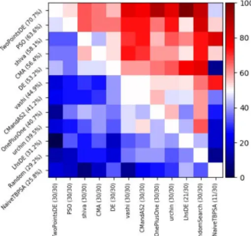
We here consider tests which are not directly from YABBOB vari-ants. Some functions are common to some of YABBOB; this section, as opposed to the next one, is not intended to be a completely independent test: these tests are either related to YABBOB or to real world tests from the next section. This section illustrates the behavior of Shiwa on various families of functions, for analysis purposes. Results are presented in Fig. 4, 5 and 6 and 7.T and d in the captions refer to the computational budget and dimension, respectively. We keep the name of these experiments as in [46]. The context of Fig. 7 (“illcondi” problem in Nevergrad) is as fol-lows: smooth ill-conditioned problems, namely Cigar and Ellipsoid,

both rotated and unrotated, in dimension 50 with moderate com-putational budget (from 100 to 10000). Unsurprisingly, for these problems for which ruggedness is null and the challenge is to tackle ill-conditioning within a moderate computational budget, SQP and Cobyla outperform all methods based on random exploration: Shiwa (and its variant Urchin) can compete, without knowing anything about the objective functions, because, based on the low computa-tional budget it switches to a chaining of CMA and Powell or to Cobyla (depending on the budget, see Fig. 1), and not to classical evolutionary methods alone.

(7)

(a) Parallel Multimodal (1000 parallel workers). (b) SPSA test: noisy benchmark designed for testing Simultaneous Per-turbation Stochastic Approximation (SPSA) [47].

Figure 6: We here plot results on other specific homogeneous families of problems (Fig. 5 continued).

Figure 7: Ill-conditioned optimization (“illcondi” in [46]). Here this is a big gap between the top algorithms and others - evolutionary algorithms are not competitive on smooth

ill-conditioned functions.

3.4 Testing: real world testbeds

We test our method on the “realworld” collection of problems in [46]. This contains Traveling Salesman Problems (TSPs), Power Sys-tems Management, Photonics, ARCoating (design of anti-reflective coatings in optics [13]), Machine Learning and Data Applications (MLDA [20]), Games (policy optimization, incl. non-metrizable do-mains). Results are presented in Fig. 8, and problems in this figure are all independent of YABBOB variants which were used for fine-tuning Shiwa. Photonics and ARCoating problems are one of our contributions. The Photonics problems are truly evolutionary in

Figure 8: Test on real-world problems, in the “realworld” benchmark from Nevergrad. This single figure aggregates many real world problems from [46] as documented there - here Shiwa outperforms most competitors because it

per-forms decently on all subfamilies of problems. This testbed contains 21 different functions, tested over 3 different de-grees of parallelism, and many distinct budgets. Urchin is a variant of Shiwa.

the sense that the best solutions correspond to optical structures which occur in nature [3] and have thus been produced by evo-lution. These testbeds are characterized by a very large number of local minima because these structures present potentially a lot of resonances. Finally, these problems are particularly modular, the different parts of the structures playing different roles without being truly independent.

4 CONCLUSIONS

We designed Shiwa (Section 2.4.2), a versatile optimization algo-rithm tackling optimization problems on arbitrary domains (con-tinuous or discrete or mixed), noisy or not, parallel or oneshot or sequential, and outperforming many methods thanks to a combi-nation of a wide range of optimization algorithms. The remarks in

(8)

Figure 9: Test on photonics problems, namely Bragg, Mor-pho and Chirped. This experiment is one of our contribu-tions: it combines sequential and 50-parallel experiments, with dimension ranging from 60 to 80 and computational budget from 100 to 10000. Urchin is a slightly modified clone of Shiwa.

Section 2.4.1, namely comparisons between optimizers over various domains, have scientific value by themselves, and are not visible in many existing testbeds. Experimental results include artificial ones: these results on YABBOB could be biased given that results on YABBOB were used for designing Shiwa. But the results are also good on variants of YABBOB which were not used for designing the algorithms (Fig. 3), and on a wide real-world public testbed, namely “realworld” from Nevergrad, and on our new Photonics implementation. Results were particularly good for wide families of problems, for which no homogeneous method alone can perform well. Shiwa can also take into account the presence of noise (with-out knowledge of the noise intensity, rarely available in real life), type of variables, computational budget, dimension, parallelism, for extracting the best of each method and outperforming existing methods. As an example of versatility, Shiwa outperforms CMA on YABBOB, is excellent on real world benchmarks, on the new photonics problems, and on ill-conditioned quadratic problems, and outperforms most one-shot optimization methods. In Fig. 8, cover-ing a wide range of problems which have never been used in the design of Shiwa, Shiwa performed well. Reproducibility matters: all our code is integrated in [46] and publicly available. Limitations. We met classes of functions for which we failed to become better on the first, without degrading on the second. Typically, we are happy with the results in parallel, one-shot, high-dimensional or ill-conditioned cases: we get good results for any of these cases, without degrading more classical settings. The extension to noisy

cases or discrete cases was also straightforward and without draw-back. But for hard multimodal settings vs ill-conditioned unimodal functions, we did our best to choose a realistic compromise but could not have something optimal for both. The no-free lunch [52] actually tells us that we can not be universally optimal. Additional research in the active selection part might help.

Further work. 1. We consider taking into account, as a prob-lem feature, the computational cost of the objective function, the presence of constraints, and, in particular for being more versa-tile regarding multimodal vs monomodal problems and rugged vs smooth problems, using more active (i.e. online) portfolios, or fitness analysis. 2. A challenge is to recursively analyze the do-main for combining different algorithms on different groups of variables: this is in progress. 3. Splitting algorithms are present in [46]. We feel that they are quite good in high dimension and could be part of Shiwa. 4. Particle Swarm Optimization is excellent in some difficult cases: we try to leverage it by integrating it into Shiwa. 5. We did not present our experiments in discrete settings: they can however be retrieved in the section entitled “wide-discrete” of http://dl.fbaipublicfiles.com/nevergrad/allxps/list.html. We see there the good performance of tools using softmax, including Shiwa. We did not include this in the present paper because, in the context of limited space, there was not enough diversity in the experiments. A thorough analysis of this method, rather new and beyond the scope of the present work dedicated to algorithm selection, is left as further work. 6. Shiwa was mainly designed by scientific knowl-edge, and a bit by trial-and-error on YABBOB. We guess much better results could be obtained by a more systematic analysis, e.g. numer-ical optimization on a wider counterpart of YABBOB. 7. Integrating e.g. [33] for high-dimensional cases is also a possibility.

ACKNOWLEDGMENTS

Author J. Liu was supported by the National Key R&D Pro-gram of China (Grant No. 2017YFC0804003), the National Natural Science Foundation of China (Grant No. 61906083), the Guang-dong Provincial Key Laboratory (Grant No. 2020B121201001), the Program for Guangdong Introducing Innovative and Enter-preneurial Teams (Grant No. 2017ZT07X386), the Science and Tech-nology Innovation Committee Foundation of Shenzhen (Grant No. JCYJ20190809121403553), the Shenzhen Science and Technology Program (Grant No. KQTD2016112514355531) and the Program for University Key Laboratory of Guangdong Province (Grant No. 2017KSYS008).

REFERENCES

[1] Artelys. 2019. Artelys Knitro, winner of the 2019 BBComp edition. https: //www.artelys.com/news/solvers-news/knitro-bbcomp-winner/

[2] Emanouil I Atanassov. 2004. On the discrepancy of the Halton sequences. Math. Balkanica (NS) 18, 1-2 (2004), 15–32.

[3] Mamadou Aliou Barry, Vincent Berthier, Bodo D. Wilts, Marie-Claire Cam-bourieux, Rémi Pollés, Olivier Teytaud, Emmanuel Centeno, Nicolas Biais, and Antoine Moreau. 2018. Evolutionary algorithms converge towards evolved bio-logical photonic structures. arXiv:1808.04689 [physics.optics]

[4] Nicolas Baskiotis and Michèle Sebag. 2004. C4.5 competence map: a phase transition-inspired approach. In Machine Learning, Proceedings of the Twenty-first International Conference (ICML 2004), Banff, Alberta, Canada, July 4-8, 2004. [5] H.-G. Beyer. 2001. The Theory of Evolution Strategies. Springer, Heideberg. [6] Hans-Georg Beyer. 2012. http://lists.lri.fr/pipermail/bbob-discuss/2012-April/

000270.html.

[7] Hans-Georg Beyer. 2012. http://lists.lri.fr/pipermail/bbob-discuss/2012-April/ 000258.html.

(9)

[8] Bernd Bischl, Pascal Kerschke, Lars Kotthoff, Thomas Marius Lindauer, Yuri Malitsky, Alexandre Fréchette, Holger H. Hoos, Frank Hutter, Kevin Leyton-Brown, Kevin Tierney, and Joaquin Vanschoren. 2016. ASlib: A Benchmark Library for Algorithm Selection. Artificial Intelligence (AIJ) 237 (2016), 41 – 58. https://doi.org/10.1016/j.artint.2016.04.003

[9] Peter AN Bosman and Dirk Thierens. 2000. Expanding from Discrete to Continu-ous Estimation of Distribution Algorithms: The IDEA. In International Conference on Parallel Problem Solving from Nature. Springer, 767–776.

[10] Sébastien Bubeck, Rémi Munos, and Gilles Stoltz. 2011. Pure exploration in finitely-armed and continuous-armed bandits. Theor. Comput. Sci. 412, 19 (2011), 1832–1852.

[11] M. L. Cauwet, C. Couprie, J. Dehos, P. Luc, J. Rapin, M. Riviere, F. Teytaud, and O. Teytaud. 2019. Fully Parallel Hyperparameter Search: Reshaped Space-Filling. Arxiv eprint 1910.08406 (2019).

[12] Marie-Liesse Cauwet, Jialin Liu, Baptiste Rozière, and Olivier Teytaud. 2016. Algorithm portfolios for noisy optimization. Annals of Mathematics and Artificial Intelligence 76, 1-2 (2016), 143–172.

[13] Emmanuel Centeno, Amira Farahoui, Rafik Smaali, Angélique Bousquet, François Réveret, Olivier Teytaud, and Antoine Moreau. 2019. Ultra thin anti-reflective coatings designed using Differential Evolution. arXiv:1904.02907 [physics.optics] [14] Rémi Coulom. 2007. Computing “ELO ratings” of move patterns in the game of

Go. ICGA journal 30, 4 (2007), 198–208.

[15] Remi Coulom. 2012. http://lists.lri.fr/pipermail/bbob-discuss/2012-April/000257. html.

[16] Remi Coulom. 2012. http://lists.lri.fr/pipermail/bbob-discuss/2012-April/000252. html.

[17] Duc-Cuong Dang and Per Kristian Lehre. 2016. Self-adaptation of Mutation Rates in Nonelitist Populations. In Parallel Problem Solving from Nature PPSN XIV -14th International Conference, Edinburgh, UK, September 17-21, 2016, Proceedings. 803–813.

[18] Jérémie Decock and Olivier Teytaud. 2013. Noisy Optimization Complexity Under Locality Assumption. In Proceedings of the Twelfth Workshop on Foundations of Genetic Algorithms XII (Adelaide, Australia) (FOGA XII ’13). ACM, New York, NY, USA, 183–190.

[19] Benjamin Doerr, Huu Phuoc Le, Régis Makhmara, and Ta Duy Nguyen. 2017. Fast Genetic Algorithms. In Proceedings of the Genetic and Evolutionary Computation Conference (GECCO ’17). ACM, 777–784.

[20] Marcus Gallagher and Sobia Saleem. 2018. Exploratory Landscape Analysis of the MLDA Problem Set. In Proceedings of PPSN18 Workshops.

[21] J. M. Hammersley. 1960. Monte-Carlo Methods For Solving Multivariate Problems. Annals of the New York Academy of Sciences 86, 3 (1960), 844–874.

[22] Nikolaus Hansen, Anne Auger, Steffen Finck, and Raymond Ros. 2012. Real-Parameter Black-Box Optimization Benchmarking: Experimental Setup. Technical Report. Université Paris Sud, INRIA Futurs, Équipe TAO, Orsay, France. http: //coco.lri.fr/BBOB-downloads/download11.05/bbobdocexperiment.pdf [23] Nikolaus Hansen and Andreas Ostermeier. 1996. Adapting arbitrary normal

mutation distributions in evolution strategies: The covariance matrix adaptation. In Proceedings of IEEE international conference on evolutionary computation. IEEE, 312–317.

[24] Verena Heidrich-Meisner and Christian Igel. 2009. Hoeffding and Bernstein Races for Selecting Policies in Evolutionary Direct Policy Search. In Proceedings of the 26th Annual International Conference on Machine Learning (ICML ’09). ACM, 401–408.

[25] Michael Hellwig and Hans-Georg Beyer. 2016. Evolution Under Strong Noise: A Self-Adaptive Evolution Strategy Can Reach the Lower Performance Bound - The pcCMSA-ES. In Parallel Problem Solving from Nature – PPSN XIV, Julia Handl, Emma Hart, Peter R. Lewis, Manuel López-Ibáñez, Gabriela Ochoa, and Ben Paechter (Eds.). Springer International Publishing, Cham, 26–36. [26] John H. Holland. 1973. Genetic Algorithms and the Optimal Allocation of Trials.

SIAM J. Comput. 2, 2 (1973), 88–105.

[27] Donald R. Jones, Matthias Schonlau, and William J. Welch. 1998. Efficient Global Optimization of Expensive Black-Box Functions. Journal of Global Optimization 13, 4 (01 Dec 1998), 455–492. https://doi.org/10.1023/A:1008306431147 [28] James Kennedy and Russell C. Eberhart. 1995. Particle swarm optimization. In

Proceedings of the IEEE International Conference on Neural Networks. 1942–1948. [29] Pascal Kerschke, Holger H. Hoos, Frank Neumann, and Heike Trautmann. 2018.

Automated Algorithm Selection: Survey and Perspectives. Evolutionary Compu-tation (ECJ) (2018), 1 – 47. https://doi.org/10.1162/evco_a_00242

[30] Pascal Kerschke and Heike Trautmann. 2018. Automated Algorithm Selection on Continuous Black-Box Problems By Combining Exploratory Landscape Analysis and Machine Learning. Evolutionary Computation (ECJ) (2018), 1 – 28. https: //doi.org/10.1162/evco_a_00236

[31] Vasil Khalidov, Maxime Oquab, Jérémy Rapin, and Olivier Teytaud. 2019. Con-sistent population control: generate plenty of points, but with a bit of resam-pling. In Proceedings of the 15th ACM/SIGEVO Conference on Foundations of Ge-netic Algorithms, FOGA 2019, Potsdam, Germany, August 27-29, 2019. 116–123. https://doi.org/10.1145/3299904.3340312

[32] Lars Kotthoff. 2014. Algorithm Selection for Combinatorial Search Problems: A Survey. AI Magazine 35, 3 (2014), 48 – 60. https://doi.org/10.1609/aimag.v35i3. 2460

[33] I. Loshchilov, T. Glasmachers, and H.-G. Beyer. 2019. Large Scale Black-box Optimization by Limited-Memory Matrix Adaptation. IEEE Transactions on Evo-lutionary Computation 23, 2 (2019), 353–358. DOI: 10.1109/TEVC.2018.2855049. [34] Katherine Mary Malan and Andries Petrus Engelbrecht. 2013. A Survey of Tech-niques for Characterising Fitness Landscapes and Some Possible Ways Forward. Information Sciences (JIS) 241 (2013), 148 – 163. https://doi.org/10.1016/j.ins.2013. 04.015

[35] Olaf Mersmann, Bernd Bischl, Heike Trautmann, Mike Preuss, Claus Weihs, and Günter Rudolph. 2011. Exploratory Landscape Analysis. In Proceedings of the 13th Annual Conference on Genetic and Evolutionary Computation (GECCO) (Dublin, Ireland). ACM, 829 – 836. https://doi.org/10.1145/2001576.2001690

[36] J. Montgomery and S. Chen. 2010. An analysis of the operation of differential evolution at high and low crossover rates. In IEEE Congress on Evolutionary Computation. 1–8.

[37] Mario Andrés Muñoz Acosta, Yuan Sun, Michael Kirley, and Saman K. Halgamuge. 2015. Algorithm Selection for Black-Box Continuous Optimization Problems: A Survey on Methods and Challenges. Information Sciences (JIS) 317 (October 2015), 224 – 245. https://doi.org/10.1016/j.ins.2015.05.010

[38] Heinz Mühlenbein and Gerhard Paass. 1996. From recombination of genes to the estimation of distributions I. Binary parameters. In International conference on parallel problem solving from nature. Springer, 178–187.

[39] Maxime Oquab, Jeremy Rapin, Olivier Teytaud, and Tristan Cazenave. 2019. Paral-lel Noisy Optimization in Front of Simulators: Optimism, Pessimism, Repetitions, Population Control. In Workshop Data-driven Optimization and Applications at CEC.

[40] Martin Pelikan, David E Goldberg, and Fernando G Lobo. 2002. A survey of opti-mization by building and using probabilistic models. Computational optiopti-mization and applications 21, 1 (2002), 5–20.

[41] Erik Pitzer and Michael Affenzeller. 2012. A Comprehensive Survey on Fitness Landscape Analysis. In Recent Advances in Intelligent Engineering Systems, János Fodor, Ryszard Klempous, and Carmen Paz Suárez Araujo (Eds.). Springer, 161 – 191. https://doi.org/10.1007/978-3-642-23229-9_8

[42] M. J. D. Powell. 1964. An efficient method for finding the minimum of a function of several variables without calculating derivatives. Comput. J. 7, 2 (1964), 155–162. [43] M. J. D. Powell. 1994. A Direct Search Optimization Method That Models the Objective and Constraint Functions by Linear Interpolation. Springer Netherlands, Dordrecht, 51–67.

[44] N. J. Radcliffe and P. D. Surry. 1994. Formal memetic algorithms. In Evolutionary Computing: AISB Workshop, T.C. Fogarty (Ed.). Springer Verlag LNCS 865, 1–16. [45] Jérémy Rapin, Pauline Dorval, Jules Pondard, Nicolas Vasilache, Marie-Liesse Cauwet, Camille Couprie, and Olivier Teytaud. 2019. Openly revisiting derivative-free optimization. In Proceedings of the Genetic and Evolutionary Computation Conference Companion, GECCO 2019, Prague, Czech Republic, July 13-17, 2019, Manuel López-Ibáñez, Anne Auger, and Thomas Stützle (Eds.). ACM, 267–268. https://doi.org/10.1145/3319619.3321966

[46] J. Rapin and O. Teytaud. 2018. Nevergrad - A gradient-free optimization platform. https://GitHub.com/FacebookResearch/Nevergrad.

[47] Pushpendre Rastogi, Jingyi Zhu, and James C. Spall. 2016. Efficient implementa-tion of enhanced adaptive simultaneous perturbaimplementa-tion algorithms. In 2016 Annual Conference on Information Science and Systems, CISS 2016, Princeton, NJ, USA, March 16-18, 2016. 298–303.

[48] John Rischard Rice. 1976. The Algorithm Selection Problem. Advances in Com-puters 15 (1976), 65 – 118. https://doi.org/10.1016/S0065-2458(08)60520-3 [49] Kate Amanda Smith-Miles. 2009. Cross-Disciplinary Perspectives on

Meta-Learning for Algorithm Selection. ACM Computing Surveys (CSUR) 41 (January 2009), 1 – 25. https://doi.org/10.1145/1456650.1456656

[50] Rainer Storn and Kenneth Price. 1997. Differential evolution–a simple and efficient heuristic for global optimization over continuous spaces. Journal of Global Optimization 11, 4 (1997), 341–359.

[51] Yizao Wang, Jean-Yves Audibert, and Rémi Munos. 2009. Algorithms for infinitely many-armed bandits. In Advances in Neural Information Processing Systems. 1729– 1736.

[52] D. H. Wolpert and W. G. Macready. 1997. No free lunch theorems for optimization. IEEE Transactions on Evolutionary Computation 1, 1 (April 1997), 67–82. https: //doi.org/10.1109/4235.585893