Analysis and Modeling of Airport Surface
Operations
by
Harshad Khadilkar
Submitted to the Department of Aeronautics and Astronautics
in partial fulfillment of the requirements for the degree of
Master of Science in Aeronautics and Astronautics
at the
MASSACHUSETTS INSTITUTE OF TECHNOLOGY
June 2011
c
Massachusetts Institute of Technology 2011. All rights reserved.
Author . . . .
Department of Aeronautics and Astronautics
May 07, 2011
Certified by . . . .
Hamsa Balakrishnan
Assistant Professor of Aeronautics and Astronautics
Thesis Supervisor
Accepted by . . . .
Eytan H. Modiano
Associate Professor of Aeronautics and Astronautics
Chair, Graduate Program Committee
Analysis and Modeling of Airport Surface Operations
by
Harshad Khadilkar
Submitted to the Department of Aeronautics and Astronautics on May 07, 2011, in partial fulfillment of the
requirements for the degree of
Master of Science in Aeronautics and Astronautics
Abstract
The focus of research in air traffic control has traditionally been on the airborne flight phase. Recently, increasing the efficiency of surface operations has been recognized to have significant potential benefits in terms of fuel and emissions savings. To iden-tify opportunities for improvement and to quaniden-tify the consequent gains in efficiency, it is necessary to characterize current operational practices. This thesis describes a framework for analysis of airport surface operations and proposes metrics to quan-tify operational performance. These metrics are then evaluated for Boston Logan International Airport using actual surface surveillance data. A probabilistic model for real-time prediction of aircraft taxi-out times is described, which improves upon the accuracy of previous models based on queuing theory and regression. Finally, a regression model for estimation of aircraft taxi-out fuel burn is described. Together, the modules described here form the basis for a surface operations optimization tool that is currently under development.
Thesis Supervisor: Hamsa Balakrishnan
Acknowledgments
The authors would also like to acknowledge regular inputs provided by Prof. John Hansman, Dr. Richard Jordan, Dr. Mariya Ishutkina and Dr. Tom Reynolds from MIT/Lincoln Laboratory and Brendan Reilly from the FAA. In addition, we also thank Jim Eggert and Daniel Herring from MIT Lincoln Laboratory for their help with setting up the ASDE-X data transfer process.
On a personal note, I would like to acknowledge the able guidance, ideas and motiva-tion provided by my advisor Prof. Hamsa Balakrishnan. A big thank you goes out to all my ICAT colleagues, in particular Ioannis Simaiakis, Varun Ramanujam, Diana Michalek-Pfeil, Hanbong Lee, Juan Jose Rebollo, Alex Donaldson and Lishuai Li for constant feedback and suggestions. Specifically, parts of Chapter 3 were worked on in close collaboration with Ioannis Simaiakis. Last but not least, I thank my parents, family and friends for their continued support, advice and encouragement.
Contents
1 Introduction 17
1.1 Motivation . . . 17
1.2 Thesis Development . . . 18
2 ASDE-X Data Preprocessing 21 2.1 Introduction . . . 21
2.1.1 Motivation . . . 21
2.1.2 Overview of ASDE-X data . . . 22
2.2 Formulation . . . 23
2.2.1 System Dynamics . . . 23
2.2.2 Form of filter . . . 26
2.3 Results . . . 30
2.3.1 Multi-Modal Filter Output . . . 30
2.3.2 Comparison with single-mode UKF and Raw data . . . 36
2.4 Summary . . . 37
3 Characterization of Airport Surface Operations 39 3.1 Introduction . . . 39
3.2 Airport Operational Characteristics . . . 40
3.2.1 Departure Queue Characteristics . . . 40
3.2.2 Departure Throughput Characteristics . . . 42
3.3 Operational Performance Metrics . . . 42
3.3.2 Runway Utilization . . . 44
3.3.3 Departure Spacing Efficiency . . . 49
3.4 Performance Metrics: Operational Feedback . . . 53
3.5 Summary . . . 54
4 Taxi Time Prediction 55 4.1 Introduction . . . 55
4.1.1 Motivation . . . 55
4.1.2 Prediction Model Overview . . . 56
4.2 Model Development . . . 56
4.2.1 Model Structure . . . 56
4.2.2 Analysis of Empirical Data . . . 58
4.2.3 Link Travel Time Model . . . 59
4.3 Results . . . 61
4.3.1 Aggregate Predictions . . . 61
4.3.2 Traffic-dependent parameters . . . 65
4.3.3 Taxi-out time predictions . . . 66
4.3.4 Prediction accuracy for complete taxi-out times . . . 70
4.3.5 Recommendation of taxi-out start times . . . 71
4.4 Summary . . . 72
5 Fuel Burn Modeling 73 5.1 Introduction . . . 73
5.1.1 Problem Description . . . 74
5.1.2 FDR Database . . . 75
5.2 Data Analysis Algorithms . . . 76
5.2.1 Preprocessing . . . 76
5.2.2 Baseline Fuel Consumption . . . 76
5.2.3 Events of Interest during Taxi-out . . . 78
5.3.1 Model 1: Taxi time, number of stops and number of turns as
independent variables . . . 81
5.3.2 Model 2: Taxi time and number of acceleration events as inde-pendent variables . . . 84
5.4 Summary . . . 88
5.4.1 Discussion of results . . . 88
6 Estimation of Surface Trajectory Fuel Burn 89 6.1 Introduction . . . 89
6.2 Fuel Burn Estimates from ASDE-X Tracks . . . 89
6.3 Fuel Burn Prediction . . . 91
6.4 Summary . . . 94
List of Figures
2-1 Sample output from Multi-modal Filter . . . 31
2-2 Sample MMF output . . . 32
2-3 Taxi mode detection for a sample flight . . . 33
2-4 Comparison of raw data and filtered output for a sample flight with noise seen in position measurement . . . 34
2-5 Comparison of raw data and filtered output for a sample flight with noise seen in heading and velocity measurement . . . 35
2-6 Autocorrelation of residuals for a single sample flight . . . 35
2-7 Sample result from single-mode UKF: Raw data in white, UKF output in yellow . . . 36
2-8 Comparison of taxi-out distance ratios . . . 37
3-1 Satellite image of BOS . . . 41
3-2 Variation of mean time spent in the departure queue with departure queue length at the time of a flight joining it . . . 41
3-3 Departure throughput saturation: 22L, 27 | 22R configuration. . . 43
3-4 Variation of average taxi-out times on Dec 09, 2010 . . . 45
3-5 Variation of average taxi-out times on Dec 09, 2010, including flights with EDCTs. . . 45
3-6 Utilization of Runway 9/27 on Dec 09, 2010 . . . 47
3-7 Utilization of Runway 15R/33L on Dec 09, 2010 . . . 48
3-8 Utilization of Runway 4L/22R on Dec 09, 2010 . . . 49
3-10 Departure spacing efficiency on Dec 09, 2010, accounting for the effect
of arrivals on the same/crossing runway. . . 52
3-11 Departure spacing efficiency on Dec 09, 2010, not accounting for the effect of arrivals on the same/crossing runway. . . 53
3-12 Average Departure Spacing Efficiency in common configurations . . . 54
4-1 Layout of BOS . . . 57
4-2 Network layout of BOS . . . 57
4-3 Network layout for departures from Runway 33L. . . 58
4-4 Flowchart for measuring empirical distribution of link travel times. . . 58
4-5 Distribution of taxi velocity over the link 1→2. . . 59
4-6 Unimpeded travel time over the link 1→2. . . 60
4-7 Distribution of number of stops over the link 1→2. . . 60
4-8 Distribution of stop times over the link 1→2. . . 60
4-9 Component conditional distributions for travel over link 1→2 . . . 63
4-10 Comparison of travel time distributions with 0 stops . . . 63
4-11 Comparison of travel time distributions with 1 stop . . . 63
4-12 Comparison of travel time distributions with 2 stops . . . 64
4-13 Comparison of full travel time distributions over link 1→2 . . . 64
4-14 Variation of travel times over link 1→2 with traffic on the surface. . . 65
4-15 Variation of stopping probability over link 1→2 as a function of the departure traffic on the surface. . . 67
4-16 Variation of stopping probability over link 5→7 as a function of the departure traffic on the surface. . . 67
4-17 Prediction of taxi-out times on Nov 24, 2010 using static means . . . 69
4-18 Prediction of taxi-out times on Nov 24, 2010 using dynamic means . . 70
4-19 Distribution of full taxi-out time prediction error from 20 test days, for departures from Runway 33L. . . 71
4-20 Improvement in error variance along successive nodes on a taxi-out path 71 4-21 Recommendation of taxi-out start time for a sample flight. . . 72
5-1 Comparison of fuel burn index as calculated from FDR data and that
obtained from ICAO. . . 77
5-2 Plot of heading history for one flight . . . 78
5-3 Flight with a single stop . . . 80
5-4 Flight with three stops . . . 80
5-5 A320: Simultaneous plot of velocity, fuel consumption rate and engine thrust settings . . . 84
5-6 A319: Simultaneous plot of velocity, fuel consumption rate and engine thrust settings . . . 85
5-7 Regression for the Avro-RJ 85 using number of acceleration events . . 86
5-8 Regression for the Boeing 777 using number of acceleration events . . 87
5-9 Residuals from the estimation of fuel consumption for the B777 . . . 87
5-10 Autocorrelation of residuals for the B777 . . . 87
6-1 Sample ASDE-X flight track from Nov 24, 2010 . . . 90
6-2 Velocity history for sample flight track . . . 91
6-3 Regression to acceleration events (all queues) . . . 93
6-4 Regression to acceleration events (Runway 33L) . . . 93
List of Tables
2.1 List of taxi modes . . . 25
2.2 Color coding for Figures 2-1 and 2-2 . . . 30
3.1 Target departure separations . . . 50
4.1 Parameter ranges for theoretical distributions. . . 62
4.2 Parameter values for some sample links. . . 65
5.1 Aircraft types and Engines . . . 75
5.2 Dataset update rates . . . 76
5.3 Regression Results: Number of Stops and Turns . . . 82
5.4 Regression Results: Acceleration events . . . 86
Nomenclature
ASDE-X Airport Surface Detection Equipment, Model-X ASPM Aviation System Performance Metrics
ASQP Airline Service Quality Performance system MMF Multi-Modal (Unscented Kalman) Filter UKF Unscented Kalman Filter
ICAO International Civil Aviation Organization FDR Flight Data Recorder
MTOW Maximum TakeOff Weight X Position (meters east) Y Position (meters north) V Taxi speed (m/s) θ Heading (degrees)
af Acceleration value (m/s2) in process model of filter f
ωf Turn rate value (deg/s) in process model of filter f
¯
w Process noise ¯
v Measurement noise σ2
wA Assumed process noise variance of quantity A
σvA2 Assumed measurement noise variance of quantity A P Sigma point generator matrix
Q Process noise covariance matrix
Qd Discrete equivalent process noise covariance matrix
R Measurement noise covariance matrix wc,i Sigma-point weights for covariance update
wm,i Sigma-point weights for mean update
ˆ ¯
x Estimated state vector ¯
y Actual measurement vector ˆ
¯
y Estimated measurement vector ¯
x(i) ith sigma point
Ts Measurement time step
Tamb Ambient temperature
f Total fuel consumed during taxi-out t Taxi-out time
ns Number of stops
nt Number of turns
Chapter 1
Introduction
1.1
Motivation
The field of air transportation has been a topic of intense research in recent years. The focus of this scrutiny has been on the financial aspects of the airline industry, the alleviation of delays to passengers, more efficient air traffic control procedures, and aircraft fuel burn and emissions. Efficient surface operations are a relatively new field of interest. However, there is increasing awareness of the significant benefits that research in this area can offer. Departure operations at airports are the most susceptible to delay, due to downstream constraints in the airspace, and stand to benefit the most from improved procedures and technologies. Therefore, in this thesis, we have tried to develop a picture of the current state of airport surface operations in general, and taxi-out procedures in particular. In order to truly understand the departure process, it is necessary to have access to detailed data relating to aircraft operations. Traditionally, such data has been available for airborne operations, but not for surface operations. Fortunately, the recent introduction of surface surveillance equipment such as the Airport Surface Detection Equipment, Model-X (ASDE-X) [1] in major US airports (29 as of November 2010) has solved this problem. We were able to access this data through the MIT Lincoln Laboratory’s Runway Status Lights system. A major part of this thesis will focus on leveraging archived ASDE-X data for analysis of surface operations and for prediction of aircraft behavior on the ground.
1.2
Thesis Development
While ASDE-X data offers tremendous opportunities for development of efficient pro-cedures and assessment of potential benefits, it comes with its own challenges. The detailed nature of the data means that archived files are large, with each day’s data occupying approximately 2GB of disk space. Therefore, identifying and sorting indi-vidual flight tracks is difficult. This is further complicated by exogenous tracks in the data, which may be produced by helicopters, aircraft being towed, or ground vehicles with transponders. Finally, the raw data also contains a large amount of noise. This means that a large amount of preprocessing is required before the surface surveillance data can be used for further analysis.
Consequently, Chapter 2 describes a multi-modal Unscented Kalman Filter de-veloped for estimation of aircraft position, velocity and heading from noisy surface surveillance data. The raw data is composed of tracks generated by the Airport Surface Detection Equipment, Model-X at Boston Logan International Airport. The multi-modal filter formulation facilitates estimation of aircraft taxi mode, described by different acceleration and turn rate values, in addition to aircraft states. The re-sulting sorted and smoothed flight tracks are used for the analysis described in the two subsequent chapters.
Chapter 3 describes how airport performance characteristics such as departure queue dynamics and throughput can be measured using surface surveillance data. Several metrics to measure the daily operational performance of an airport are also proposed and evaluated. The results presented are for the specific case of Boston Logan International Airport.
The accurate prediction of aircraft taxi-out times is the first step toward the optimization of departure operations at airports. In Chapter 4, we present a taxi-out time prediction tool that models the airport surface as a network. Travel times along links of the network are assumed to be random variables with unknown distributions. The methodology used to derive these distributions from empirical surface surveillance data is described. The resulting theoretical model is validated using observations from
an independent test data set, and is shown to predict taxi-out times accurately. The resultant airport surface model lends itself to use with existing route optimization algorithms with minor modifications.
In addition to ASDE-X data, we also had access to a limited amount of Flight Data Recorder (FDR) data. In addition to position and velocity, this data set also contains information on instantaneous fuel flow rate. Chapter 5 uses the FDR data to build a model for estimation of on-ground fuel consumption of an aircraft, given its surface trajectory. This model is an important part of any procedure that optimizes departure operations as it allows the assessment of potential fuel savings. Since the taxi-out phase of a flight accounts for a significant fraction of total fuel burn for aircraft, reduced taxi-out times will result in reduced CO2 emissions in the vicinity
of airports. In Chapter 5, taxi-out fuel burn is modeled as a linear function of several factors including the taxi-out time, number of stops, number of turns, and number of acceleration events. The parameters of the model are estimated using least-squares regression. The statistical significance of each of these factors is investigated. Since these factors are estimated using data from operational aircraft, they provide more accurate estimates of fuel burn than methods that use idealized physical models of fuel consumption based on aircraft velocity profiles, or the baseline fuel consumption estimates provided by the International Civil Aviation Organization. Our analysis shows that in addition to the total taxi time, the number of acceleration events is a significant factor in determining taxi fuel consumption.
Finally, Chapter 6 describes a method for applying the model to the estimation of fuel burn for flight tracks generated from surface surveillance data. A procedure that could be used to estimate fuel burn benefits from congestion management strategies is also suggested. Chapter 7 summarizes the important findings in this thesis, and suggests directions for future work.
Chapter 2
ASDE-X Data Preprocessing
The two sets of data (ASDE-X and FDR) used in this work are in time-series format. At every time step, individual aircraft states are reported. Sorting and concatenating several successive reports from the same aircraft generates flight tracks. However, the tracks thus generated contain a significant proportion of noise. Therefore, both sets of data require filtering. The noise content in FDR data is fairly low, since all the states are measured using onboard equipment. Consequently, it is sufficient to pre-process FDR data using a linear Kalman Filter. The ASDE-X data, on the other hand, contains much more noise, since it is measured using onboard transponders as well as surface surveillance equipment. Therefore, much more elaborate filtering is required to make it usable for further analysis. This chapter describes the filter developed to pre-process ASDE-X data.
2.1
Introduction
2.1.1
Motivation
The availability of surface surveillance data allows us to visualize actual taxi routes of aircraft and to directly measure metrics such as total taxi distance, taxi time and time spent in the departure queue. These quantities form the basis for further studies such as the calculation of total fuel burn due to airport surface operations [2] or the
prediction of aircraft taxi-out times [3].
However, estimates produced using raw ASDE-X tracks are prone to error, be-cause of inherent noise in the data. For example, noise in position data can lead to overestimation of taxi distance, noise in velocity data can lead to errors in detection of takeoff and landing, and noise in heading data can lead to false turn detection. In order to mitigate these effects, an unscented Kalman filter (UKF) [4, 5] in the multi-modal form was found to work very well. A bank of UKFs filters the raw data, with each filter representing a different taxi mode. The current taxi mode is detected by selecting the filter with the least (normalized) squared error, combined with a heuristic that offers resistance to rapid mode jumping.
The performance of the linear and extended versions of the Kalman filter [6] was also measured. The linear filter had insufficient noise suppression, while the extended Kalman filter was found to diverge often when applied to the current system. The unscented Kalman filter, on the other hand, was seen to be much more stable. Finally, the multi-modal filter formulation (MMF) was used because of its tracking accuracy and the relative ease of inferring taxi mode, when compared to a single filter. The multi-modal formulation has been previously used in areas such as computer vision [7], but it appears to have not been used for aircraft position tracking on the ground. The latter part of this chapter compares the performance of the MMF with a single-mode UKF.
2.1.2
Overview of ASDE-X data
The Airport Surface Detection Equipment, Model-X is primarily a safety tool de-signed to mitigate the risk of runway collisions [1]. It incorporates real-time tracking of aircraft on the surface to detect potential conflicts. There is potential, however, to use the data generated by it for surface operations analysis and aircraft behavior prediction. The data itself is generated by sensor fusion from three primary sources: (i) Surface movement radar, (ii) Multilateration using onboard transponders, and (iii) GPS-enabled Automatic Dependent Surveillance Broadcast (ADS-B). Reported parameters include each aircraft’s position, velocity, altitude and heading. The
up-date rate is of the order of 1 second for each individual track. The coverage range is approximately 20 miles out from the airport.
All the ASDE-X data used here is from the Runway Status Lights (RWSL) system at Boston Logan International Airport (BOS). The results presented in this chapter are based on data from August to December 2010. As discussed above, the raw data contains a substantial amount of noise despite an upgrade installed in April 2010 to the system at Boston.
2.2
Formulation
As mentioned in the previous section, both the linear and the extended versions of the Kalman filter were tried without much success. The linear filter was unable to reduce noise to a satisfactory level without sacrificing accuracy, while the extended filter was prone to divergence. While ‘truth’ was not available in this study since the data was from actual operations, some idea of taxi path could be inferred from the raw trajectories superimposed over a layout of the taxiways in Google Earth R.
Specifi-cally, aircraft do not stray far from the centerlines marked on the taxiways/runways, allowing comparison of filter tracking behavior by visual inspection.
2.2.1
System Dynamics
The state vector to be estimated consists of aircraft position (X in meters east and Y in meters north), absolute velocity (V , m/s) and heading (θ, degrees):
¯ x = h X Y V θ i0 (2.1)
The number of states is n = 4. To account for values of longitudinal acceleration and turn rate different from those in the system model, the velocity and heading states were assumed to have independent, zero mean, white Gaussian process noise with variance σwV2 and σ2wθ respectively. The assumption of independence meant that the
process noise covariance matrix Q was diagonal: Q = σ2 wV 0 0 σwθ2 (2.2)
Since all four states are available in ASDE-X data, the measurement vector ¯y had the same components as the state vector. It was assumed that noise variance involved in the measurement of X and Y positions was independent but had equal variance. The position, velocity and turn-rate noise variances were assumed to be equal to σvxy2 , σ2
vV and σ2vθ respectively. The measurement noise covariance matrix, R was therefore
given by: R = σ2 vxy 0 0 0 0 σ2 vxy 0 0 0 0 σ2 vV 0 0 0 0 σ2 vθ (2.3)
Finally, the continuous nonlinear state dynamics were assumed to be:
˙¯ x = ˙ X ˙ Y ˙ V ˙ θ = V sin θ V cos θ a ω + Bww¯ (2.4)
Here, a is the longitudinal acceleration and ω is the turn rate, both of which are assigned different constant values in the system model for each mode. Since a heading of zero degrees is due north, the sine component of velocity affects X position while the cosine component affects Y position. A full list of taxi modes is given in Table 2.1. For the single-mode UKF used for comparison purposes, the assumed values were a = ω = 0. The additive noise term in (2.4) is the product of the the matrix Bw and
the process noise ¯w. The noise vector ¯w = [wV wθ]0 contains noise in acceleration
affects only velocity and turn rate, and is given by: Bw = 0 0 0 0 1 0 0 1 (2.5)
The measurement vector is equal to the state vector with an additive noise term:
¯
y = ¯x + ¯v (2.6)
Here ¯v = [vX vY vV vθ]0 is the measurement noise vector, assumed to be
inde-pendent of process noise, white, Gaussian and to vary like N (0, R). The diagonal covariance matrix R ensures that the elements of measurement noise are independent of each other.
Mode Description Longitudinal Turn
Number Acceleration Rate
a (m/s2) ω (deg/s)
1 Default 0 0
2 Moderate Acceleration 1 0
3 Moderate Deceleration -1 0
4 Constant Speed Turn Right 0 10 5 Constant Speed Turn Left 0 -10 6 Accelerating Turn Right 3 10 7 Accelerating Turn Left 3 -10 8 Decelerating Turn Right -3 10 9 Decelerating Turn Left -3 -10
10 High Acceleration 3 0
11 High Deceleration -3 0
2.2.2
Form of filter
Definition of Constants
The UKF formulation used for each mode was based on the method proposed by Wan and van der Merwe [4]. According to this method, a state vector of length n results in (2n + 1) sigma points. Some additional required constants are defined below. Note that in this case, the number of states is n = 4.
κ = 3 − n (2.7a)
α = 0.5 (2.7b)
λ = α2(n + κ) − n (2.7c)
β = 2 (2.7d)
Based on these constants, the weights used for generation of the (2n + 1) sigma points from the sigma point generator matrix are defined.
wc,i = 1 2(n + λ) for i = 1, 2, ..., 2n (2.8a) wc,2n+1 = λ n + λ + 1 − α 2+ β (2.8b) wm,j = 1 2(n + λ) for j = 1, 2, ..., 2n (2.8c) wm,2n+1 = λ n + λ (2.8d)
Finally, the discrete equivalent process noise covariance matrix, Qd, is based on the
approximation (2.9), with Ts the time difference between two successive
measure-ments. Note that Qd is of size 4 × 4.
Qd≈ BwQBwTTs (2.9)
Filter Algorithm
Let us define the quantity zk(i)+ to be the value of the generic quantity z after the measurement update at time step k, for the ith sigma point where i = 1, 2, ..., 2n + 1.
Similarly, zk+1(i)− is the quantity z propagated to time step k + 1 but prior to the measurement update at time step k + 1. Let ˆx denote the estimated state vector,¯ ¯
x(i) denote the ith sigma point, ¯y denote actual measurements, ˆy be the expected¯ measurement vector and P be the sigma point generator matrix, viz. the uncertainty matrix from which sigma points are generated. The filter algorithm [4] is given below. Since all the states are available for measurement, algorithm initialization is done using ˆx¯+0 = ¯y0 (first detection of current aircraft) and P0+ = R.
1. Generation of sigma points at time step k, with the ith sigma point generated using the transpose of the ith row belonging to the matrix square root of (n +
λ)Pk+: ¯ x(i)+k = ˆx¯+k + [{ q (n + λ)Pk+}(i)]T for i = 1, 2, ..., n = ˆx¯+k − [{ q (n + λ)Pk+}(i)]T for i = (n + 1), (n + 2), ..., 2n = ˆx¯+k for i = 2n + 1
2. Propagation of belief to the next time step, with af and ωf being the acceleration
and turn rate values assumed in the system model for filter f . The propagation equations are based on simple kinematics.
¯ x(i)−k+1 = ¯x(i)+k + (Vk(i)+Ts+ 12afTs2) sin (180π θ (i)+ k ) (Vk(i)+Ts+ 12afTs2) cos ( π 180θ (i)+ k ) afTs ωfTs
3. Calculation of expected state vector at step k + 1 from the propagated sigma points: ˆ ¯ x−k+1 = 2n+1 X i=1 wm,ix¯ (i)− k+1
4. Estimation of the uncertainty covariance matrix: Pk+1− = Qd+ 2n+1 X i=1 wc,i(¯x (i)− k+1 − ˆx¯ − k+1)(¯x (i)− k+1− ˆx¯ − k+1) T
5. Recalculation of sigma points ¯x(i)−k+1 using the same equations as in step 1, but with Pk+1− as the generating matrix. The measurement sigma points, ¯y(i)k+1, are equal to ¯x(i)−k+1 since full state measurement is available.
6. Calculation of expected measurement vector at step k + 1:
ˆ ¯ yk+1 = 2n+1 X i=1 wm,iy¯ (i) k+1
7. Calculation of the Kalman filter gain at time step k + 1, Lk+1:
Pyy = R + 2n+1 X i=1 wc,i(¯y (i) k+1− ˆy¯k+1)(¯y (i) k+1− ˆy¯k+1) T Pxy = 2n+1 X i=1 wc,i(¯x (i)− k+1 − ˆx¯ − k+1)(¯y (i) k+1− ˆy¯k+1)T Lk+1 = PxyPyy−1
8. Belief update using actual measurement at time step k + 1, ¯yk+1:
ˆ ¯
x+k+1 = ˆx¯−k+1+ L · (¯yk+1− ˆy¯k+1)
This algorithm is run simultaneously on all filters in the bank. The expected measurement from each filter is compared to the actual measurement vector. Based on this comparison, the current taxi mode is set, and the state estimate from the cor-responding filter becomes the new state estimate for the entire bank. The algorithm then repeats, starting from step 1.
Selection of Taxi Mode
The selection of taxi mode is based upon a Quality Index (QI) that is essentially the negative of the second-order norm of the residual for each filter, normalized by the measurement noise covariance.
QI = −(¯yk+1− ˆy¯k+1)TR−1(¯yk+1− ˆy¯k+1) (2.10)
The filter selection algorithm tracks the Quality Index for each filter, for the latest three time steps. The particular filter selected is the one that has the maximum QI, among all f filters, for the most times in these three time steps. If three different filters have one instance each of maximum QI in the last three time steps, the incumbent filter continues to be selected. The algorithm is initiated at the start of each flight track with the ‘straight, constant velocity’ mode active.
A Gaussian likelihood estimate, based on the measurement error of each filter, and the uncertainty as derived from the matrix P , was initially tested as the criterion for mode selection. However, it was found that the measurement noise can cause the error to be occasionally so large that all likelihood values drop to machine zero. In addition, the evaluation of Gaussian likelihood requires a call to a separate subroutine in the code, and is computationally expensive. Therefore, the second-order norm was chosen as a measure of likelihood. The additional heuristic of choosing the best filter over the last three time steps helps avoid frequent mode jumping caused by erratic measurement errors.
2.3
Results
2.3.1
Multi-Modal Filter Output
A comparison of the output from the multi-modal filter with raw data is shown in Figure 2-1, while Figure 2-2 shows sample output for a departure and an arrival. Figure 2-1 is from a portion of taxiway close to the threshold of Runway 33L at Boston Logan. The white line in the upper plot traces the raw data, while the multi-colored segmented line in the lower plot is the filter output. It can be seen that most of the noise in the raw data has been filtered out by the MMF. At the same time, an idea about tracking performance of the filter can be obtained by observing that filtered output in all the figures is fairly close to the taxiway markings on the surface. Note that the colors in the filter output indicate the taxi mode as detected by the filter. Table 2.2 relates the colors to the taxi modes from Table 2.1.
Taxi Mode Mode Numbers Color
Raw data - White
Straight, constant speed 1, 2, 3 Dark Blue Decelerating straight / turn 8, 9, 11 Red Accelerating straight / turn 6, 7, 10 Green Turn, constant speed 4, 5 Light Blue
Table 2.2: Color coding for Figures 2-1 and 2-2
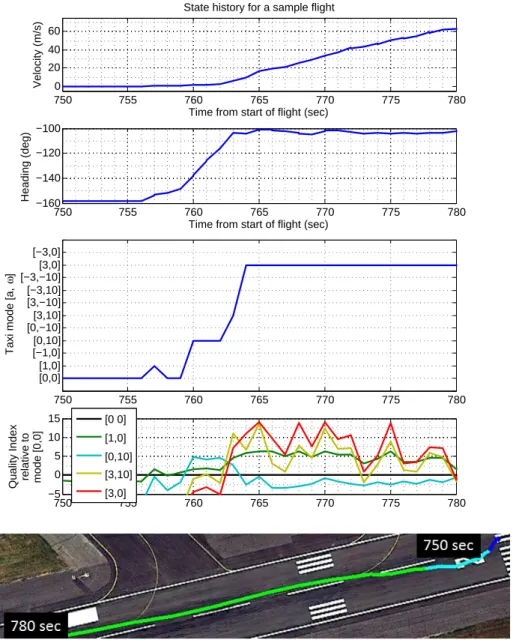
Figure 2-3 shows results from the taxi mode detection algorithm for a specific flight. It can be seen that the code correctly detects a constant speed turn (starting at 756 seconds on the X axis) followed by takeoff, which is a period of sustained high acceleration. Note that the fourth plot in the figure shows relative Quality Index values for each mode, i.e., the difference between the Quality Index of each filter and the instantaneous Quality Index of the default mode having [a, ω] = [0, 0].
(a) Raw Data
(b) MMF Output
Figure 2-1: Sample output from Multi-modal Filter. Both pictures correspond to the area enclosed by the orange rectangle in the inset image.
(a) Arriving flight: Landing on the runway is seen on the right, with strong braking marked in red. The flight then leaves the runway and taxis towards its gate beyond the top edge of the picture. Portions where a turn was detected are marked in light blue.
(b) Departing flight: Departure is on Runway 4R, with acceleration phase indicated in green.
750 755 760 765 770 775 780 0
20 40 60
Time from start of flight (sec)
Velocity (m/s)
State history for a sample flight
750 755 760 765 770 775 780
−160 −140 −120 −100
Time from start of flight (sec)
Heading (deg) 750 755 760 765 770 775 780 [0,0] [1,0] [−1,0] [0,10] [0,−10] [3,10] [3,−10] [−3,10] [−3,−10] [3,0] [−3,0]
Taxi mode [a,
ω ] 750 755 760 765 770 775 780 −5 0 5 10 15
Quality Index relative to mode [0,0]
[0 0] [1,0] [0,10] [3,10] [3,0]
Figure 2-3: Taxi mode detection for a sample flight. The first two plots show velocity and heading for the aircraft trajectory shown in the bottom plot. The third plot shows the output of the mode detection algorithm, with acceleration and turn-rate values of each mode marked on the Y axis. The fourth plot shows the quality index of the best five modes in this time period, relative to the baseline mode [a, ω] = [0, 0].
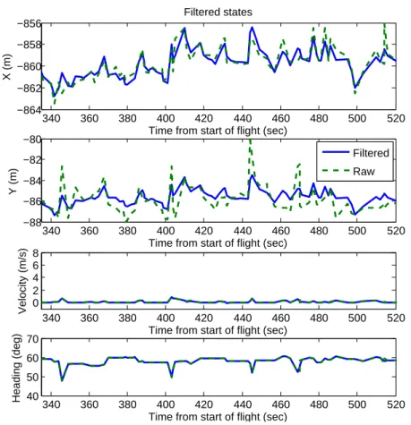
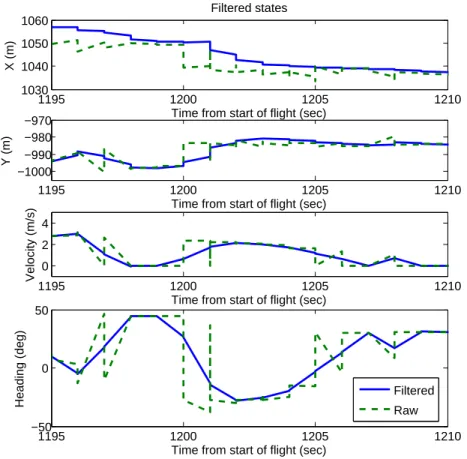
Figures 4 and 5 are typical examples of the noise in raw data. In Figure 2-4, considerable jitter is seen in the measured Y position, most of which is removed by the filter. There is some noise in the X position as well, but not much in the velocity and heading fields. In Figure 2-5, there is noise in velocity and heading but not in position. Note that each of the four fields is independently measured by the
ASDE-X system, and therefore, measured velocity is not simply the derivative of position. Finally, Figure 2-6 shows autocorrelation plots of the estimation residuals for a single flight. For each measurement variable, it shows the correlation coefficient of the residual (error) at one time step with all other residuals in the rest of the flight track. The low value of correlation except where the difference in index goes to zero (correlation with itself) indicates that the residuals are a white sequence [8, 9], and therefore the filter is working efficiently.
340 360 380 400 420 440 460 480 500 520 0 2 4 6 8
Time from start of flight (sec)
Velocity (m/s) 340 360 380 400 420 440 460 480 500 520 −864 −862 −860 −858 −856 Filtered states
Time from start of flight (sec)
X (m) 340 360 380 400 420 440 460 480 500 520 −88 −86 −84 −82 −80
Time from start of flight (sec)
Y (m) 340 360 380 400 420 440 460 480 500 520 40 50 60 70
Time from start of flight (sec)
Heading (deg)
Filtered Raw
Figure 2-4: Comparison of raw data and filtered output for a sample flight with noise seen in position measurement
1195 1200 1205 1210 1030 1040 1050 1060 Filtered states X (m)
Time from start of flight (sec)
1195 1200 1205 1210 −1000 −990 −980 −970 Y (m)
Time from start of flight (sec)
1195 1200 1205 1210
0 2 4
Time from start of flight (sec)
Velocity (m/s)
1195 1200 1205 1210
−50 0 50
Time from start of flight (sec)
Heading (deg)
Filtered Raw
Figure 2-5: Comparison of raw data and filtered output for a sample flight with noise seen in heading and velocity measurement
−4000 −2000 0 2000 4000 0 0.5 1 State 1 (X) Coefficient
Difference in index in residuals vector
−4000 −2000 0 2000 4000 0 0.5 1 State 2 (Y) Coefficient
Difference in index in residuals vector
−4000 −2000 0 2000 4000 0 0.5 1 State 3 (V) Coefficient
Difference in index in residuals vector
−4000 −2000 0 2000 4000 0 0.5 1 State 4 (θ) Coefficient
Difference in index in residuals vector
2.3.2
Comparison with single-mode UKF and Raw data
In terms of output quality, the single-mode UKF formulation ends up being inferior to the multi-modal form. This is primarily due to the fact that the process model in the single-mode UKF only accounts for straight, constant speed taxi. If noise suppression comparable to the MMF is desired, the assumed measurement noise covariance needs to be so high that the filter fails to track quick changes in velocity and heading. For example, Figure 2-7 shows the filter output belatedly tracking a turning aircraft, thus producing an estimate of position which is unrealistically close to the edge of the taxiway.
Figure 2-7: Sample result from single-mode UKF: Raw data in white, UKF output in yellow
Figure 2-8 gives an idea of the relative tracking behavior of the filters discussed so far. It shows the mean ratio of the taxi distance measured using three different meth-ods for a total of 20 flights, to the taxi distance measured visually by a straight-line approximation of the taxi path. The three ways in addition to the visual measure-ment, by which taxi distances have been calculated are (i) using the MMF, (ii) using the single-mode UKF, and (iii) from raw data. The normalization of taxi distance in this manner accounts for different taxi paths used by different flights. As seen in the figure, the mean distance measured by the MMF is closest to the straight-line
method. Note that the MMF output is likely to be closer to actual taxi distance than the straight-line approximation since aircraft do not stick strictly to taxiway centerlines. It is clear from the figure, though, that taxi distance calculated using raw data would hold very little value for further analysis, because of its large taxi distance estimates. Further, the large variance precludes the use of constant-factor scaling to increase the accuracy of the raw estimates.
Baseline Taxi Path Multi−modal UKF Single UKF Raw 1 1.2 1.4 1.6 1.8 2
Taxi distance measurement relative to total length of taxiway segments
Relative distance
Type of filter
One standard deviation Mean
Figure 2-8: Comparison of taxi-out distance ratios
2.4
Summary
In this chapter, it was showed that the raw data contained a significant amount of noise, precluding its direct application to further analysis such as taxi distance cal-culations. The MMF was shown to successfully mitigate the effect of noise, while maintaining tracking performance. Tradeoffs involved with the use of a single-mode UKF instead of the MMF were considered. It was found that the MMF had better tracking properties than the UKF, making it the filter of choice for applications re-quiring accurate estimates of aircraft position and taxi mode. In subsequent chapters, all the ASDE-X data has been pre-processed using either the single-mode UKF or the MMF, depending on the accuracy required and the amount of data to be processed.
Chapter 3
Characterization of Airport
Surface Operations
3.1
Introduction
Airports form the critical nodes of the air transportation network, and their perfor-mance is a key driver of the capacity of the system as a whole [10]. With several major airports operating close to their capacity, the smooth and efficient operation of airports is essential for the efficient functioning of the air transportation system. Studies of airport operations have traditionally focused on airline operations and on the aggregate estimation of airport capacity envelopes [11, 12, 13, 14]. Most of this research is based on data from a combination of the Aviation System Performance Metrics (ASPM) [15] and the Airline Service Quality Performance (ASQP) systems. These databases, when in individual aircraft format, provide the times at which flights pushback from their gates, their takeoff and landing times, and the gate-in times, as reported by the airlines. ASPM also provides airport-level aggregate data, which enu-merates the total number of arrivals and departures in 15-minute increments. Such data can be used to develop queuing models of airport operations [16, 17] or empiri-cally estimate airport capacity envelopes [13]. However, this level of detail is typiempiri-cally insufficient to investigate other factors that affect surface operations, such as inter-actions between taxiing aircraft, runway occupancy times, etc. As outlined in the
previous chapter, ASDE-X data does provide the level of detail that allows analysis of aircraft interaction in a disaggregate sense. This chapter describes the ways in which ASDE-X data can be leveraged to characterize airport surface operations, and proposes methods to track airport operational performance.
The filtering algorithm described in Chapter 2 processes the ASDE-X flight tracks, one full day at a time. These filtered quantities are then used to tag each valid flight track with a departure/arrival time and runway. By tracking each aircraft from pushback to wheels-off, various airport states such as the active runway configuration, location and size of the departure queue, and departure/arrival counts are measured. In addition, airport-level performance metrics such as average taxi-out times, runway usage and inter-departure spacing statistics are also tracked. The definitions of these metrics and the algorithms proposed for measuring them are described in subsequent sections of this chapter.
3.2
Airport Operational Characteristics
3.2.1
Departure Queue Characteristics
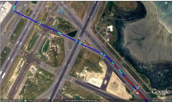
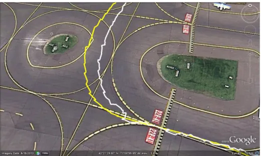
Visualization of the filtered ASDE-X data gives insights into the dynamics of airport operations. For example, locations on the surface where aircraft typically queue up for departure can be determined. These locations depend on the runway configuration and operational procedures. For example, Figure 3-1 (left) shows the layout of BOS. Figure 3-1 (right) shows the departure queues formed on a day in September 2010 in the 22L | 22R configuration, i.e., when runway 22L (on the east side) was being used for arrivals and 22R (on the west side) was being used for departures.
There is a primary departure queue at the runway threshold, and a secondary one before it. The secondary queue is composed of aircraft waiting to cross the depar-ture runway on their way to the primary queue. During the months of August and September 2010, there was taxiway construction at BOS, which closed the taxiway area denoted by white in the the figure.
Figure 3-1: (Left) Layout of Boston Logan International Airport. (Right) Visual-ization of airport operations. Aircraft in green are departures and the ones in red are arrivals. A previously arrived aircraft can be seen at the bottom of the picture, waiting to cross the departure runway on the way to its gate.
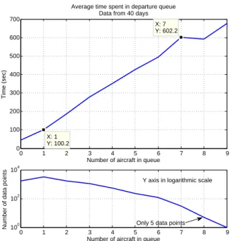
Observation of operations over several days of data provided an insight into typical queue formation areas. These areas were then designated in the analysis codes for automatic tracking of departure queues and calculation of statistics such as time spent by individual aircraft in the queue and the variation of queue length over each day. Figure 3-2 shows the variation of mean time spent in the primary departure queue,
0 1 2 3 4 5 6 7 8 9 0 100 200 300 400 500 600 700 X: 7 Y: 602.2 Average time spent in departure queue
Data from 40 days
Number of aircraft in queue
Time (sec) X: 1 Y: 100.2 0 1 2 3 4 5 6 7 8 9 100 102 104
Number of data points
Number of aircraft in queue Only 5 data points
Y axis in logarithmic scale
Figure 3-2: Variation of mean time spent in the departure queue with departure queue length at the time of a flight joining it
with the queue length. It is based on 40 days of data from all runway configurations. We define queue length as the number of aircraft in the primary departure queue as seen by a new aircraft just joining it. It can be seen that on average, each additional aircraft in queue entails a penalty of 83 seconds for all the aircraft behind it. This value seems to be reasonable when compared to the standard departure separations described in Section 3.3.3.
3.2.2
Departure Throughput Characteristics
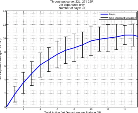
Departure queue characterization offers an insight into surface operations from an aircraft’s perspective. Airport-level operational performance was tracked using the variation of departure throughput (defined as the number of takeoffs in a 15-minute interval) with the number of active departing aircraft on the surface. Aircraft were defined to be active from the time of first transponder capture (first detection with ASDE-X) to wheels-off time. Previous studies [17, 18] have shown, using ASPM data, that the increment in departure throughput decreases with the addition of aircraft to the surface, finally leading to saturation. This is corroborated by the results pro-duced using ASDE-X data. Figure 3-3 shows the departure throughput curve for a specific configuration at Boston. Note that only jet aircraft are counted in this analysis. This is because propeller-driven aircraft are fanned out via separate depar-ture fixes at Boston, thus not affecting the jet depardepar-ture process. The throughput curves for other configurations are similar in nature to Figure 3-3, differing only in the point of saturation and maximum throughput. These differences can be attributed to configuration-specific procedures, such as closely spaced departures on intersecting runways.
3.3
Operational Performance Metrics
Building on the results described in the previous section, it is possible to develop metrics to measure an airport’s operational performance. The motivation is not to scrutinize controller performance, but to look for systematic inefficiencies and to
iden-0 2 4 6 8 10 12 14 0 2 4 6 8 10 12 14
Total Active Jet Departures on Surface (N)
Jet Departure rate (per 15 min)
Throughput curve: 22L, 27 | 22R Jet departures only Number of days: 93
Mean
One Standard Deviation
Figure 3-3: Departure throughput saturation: 22L, 27 | 22R configuration.
tify opportunities for improvement. The basic concepts used to define these metrics are generalizable to any airport. However, each airport has local rules, regulations and procedures that must be considered in order to be consistent across different con-figurations and time periods. For example, there are subtle variations in the strategies used by different airports to accommodate both arrivals and departures on the same runway or on intersecting runways. At Boston, arrivals have to cross the departure runway in the 22L, 27 | 22R configuration. On the other hand, in the 27 | 33L configuration, it is the departures that have to cross the arrival runway. Arrivals at Boston are controlled by the Boston Center, and consequently, they receive priority over departures. Their sequence and separation is not controlled by the tower. The following discussion presents the performance metrics, developed in consulation with Boston ATC, that account for as many of these complexities as possible while keeping the computational effort at a reasonable level.
3.3.1
Average Taxi-out Times
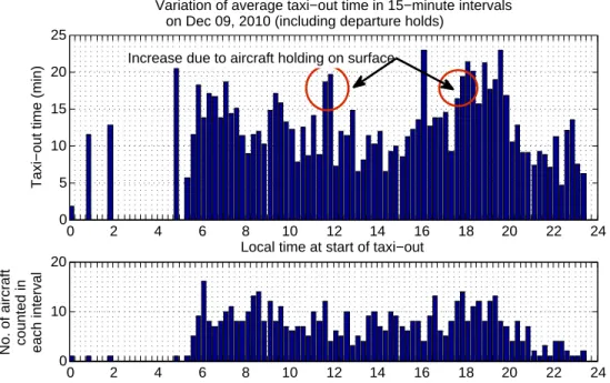
The most natural performance measure from the point of view of passengers is the average taxi-out time for departures. This is an important quantity that affects not only flight delays but also taxi-out fuel consumption. In general, taxi-out times are highest in the peak congestion periods. At Boston, these are the morning departure push at around 0600 hours local, and the evening push between 1900 and 2000 hours local time. Figure 3-4 shows the variation of average taxi-out times on a sample day. The averages are calculated over 15 minute intervals for the entire day. Each bar in the upper plot represents the average taxi-out time experienced by the aircraft pushing back in that 15 minute interval. The number of pushbacks in the corresponding interval are shown in the lower plot. The peaks in both pushbacks and taxi-out times around 0600 and 2000 can be seen clearly. Note that in the calculation of this metric, the time spent by aircraft absorbing departure holds, has been subtracted. These aircraft usually have specified departure times known as Expected Departure Clearance Times (EDCTs), decided by constraints elsewhere in the National Airspace System (NAS). While it is desirable to have aircraft absorb these delays at the gate, it is not always possible because of conflicts with arrivals that are scheduled to dock at the same gate. Figure 3-5 shows a similar plot as Figure 3-4, but with flights with EDCTs included in the data. A comparison of the two plots illustrates the effect of excluding these flights.
3.3.2
Runway Utilization
The most capacity-constrained element in departure operations is the runway [19]. Therefore, it is important to ensure that an airport’s runway system is used as effi-ciently as possible. To look at the current usage characteristics of runways at Boston, a metric called Runway Utilization was defined. The utilization is expressed as a percentage, calculated for every 15 minute interval. It is given by the fraction of time in the 15 minute interval for which a particular runway is being used for active operations. The types of active operations considered were:
0 2 4 6 8 10 12 14 16 18 20 22 24 0 5 10 15 20 25
Variation of average taxi−out time in 15−minute intervals on Dec 09, 2010 (excluding departure holds)
Taxi−out time (min)
Local time at start of taxi−out
0 2 4 6 8 10 12 14 16 18 20 22 24 0
10 20
No. of aircraft counted in each interval
Figure 3-4: Variation of average taxi-out times on Dec 09, 2010. Flights with long holds due to EDCTs have been removed from the calculation of average taxi-out times. 0 2 4 6 8 10 12 14 16 18 20 22 24 0 5 10 15 20 25
Variation of average taxi−out time in 15−minute intervals on Dec 09, 2010 (including departure holds)
Taxi−out time (min)
Local time at start of taxi−out
0 2 4 6 8 10 12 14 16 18 20 22 24 0
10 20
No. of aircraft counted in each interval
Increase due to aircraft holding on surface
Figure 3-5: Variation of average taxi-out times on Dec 09, 2010, including flights with EDCTs.
1. Departure roll: Counted from the start of takeoff roll to wheels off
2. Departure hold: A departing aircraft holding stationary on the runway, waiting for takeoff clearance
3. Approach: Counted from the time an aircraft is on short final (within 2.5 nm of runway threshold) to the time of touchdown
4. Arrival: Counted from the moment of touchdown to the time when the aircraft leaves the runway
5. Crossings/Taxi: When aircraft are either crossing an active runway, or taxiing on an inactive runway
Each of these operating modes was detected using the filtered states from ASDE-X tracks for each aircraft. The ‘approach’ phase was included in the runway utilization because no other operations can be carried out on the arrival runway, or a crossing departure runway, when an aircraft is on short final. Even though, technically, the air-craft is not on the runway, ignoring this operational constraint would give erroneously low utilization figures.
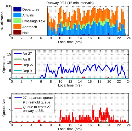
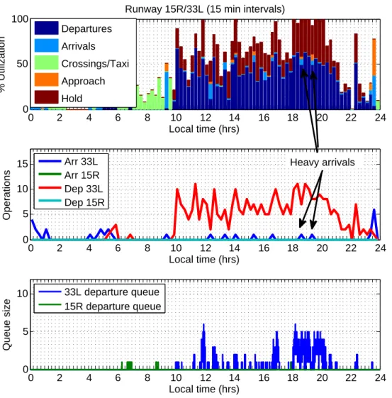
Figures 3-6 to 3-8 show the utilization plots for a sample day, for three different runways. The topmost plot in each figure shows the breakup of utilization for the runway over the course of the day. The plot in the middle shows operational counts in each 15 minute interval, for both ends of the runway. Finally, the lowermost plot shows the variation of queue length over the day. It should be noted that the queue length is calculated for every second, while the top two plots are aggregate figures over the 15 minute interval. Details such as configuration changes can be seen immediately from the utilization plots. For example, we can see from Figures 3-7 and 3-8 that departure operations shifted from runway 22R to runway 33L at 1000 hours.
Ideally, it would be desirable to have the utilization figures be 100% for the active runways in times of peak demand. The sample figures show that while this figure is achieved for much of the peak period, it is difficult to sustain. Disruptions may be caused by off-nominal events such as runway closures due to foreign objects, arrivals
0 2 4 6 8 10 12 14 16 18 20 22 24 0
50 100
Runway 9/27 (15 min intervals)
Local time (hrs) % Utilization Departures Arrivals Crossings/Taxi Approach Hold 0 2 4 6 8 10 12 14 16 18 20 22 24 0 5 10 Local time (hrs) Queue size 27 departure queue 9 threshold queue Queue to cross 27 on way to 33L 0 2 4 6 8 10 12 14 16 18 20 22 24 0 5 10 15 Local time (hrs) Operations Arr 27 Arr 9 Dep 27 Dep 9
Figure 3-6: Utilization of Runway 9/27 on Dec 09, 2010. Runway 27 was used for arrivals for the entire day. An occasional departure can be seen in the second plot, accompanied by a dip in the number of arrivals and the utilization for the time period. In the bottom plot, queue formation can be seen, composed of aircraft waiting to cross the runway for departure on 33L.
requesting a departure runway for landing, or gaps in the arrival sequence. It should be noted that the utilization for the departure runway is always higher than that for the arrival runway. This is because the departures can be packed close together, with the next aircraft in queue holding on the runway while the previous aircraft starts its climb-out. On the other hand, tightly packed arrivals increase the risk of frequent go-arounds caused by aircraft not vacating the runway quickly enough to allow the next arrival to land. Therefore, the arrival stream usually has a buffer over and above the minimum spacing dictated by standard procedures.
0 2 4 6 8 10 12 14 16 18 20 22 24 0
50 100
Runway 15R/33L (15 min intervals)
Local time (hrs) % Utilization Departures Arrivals Crossings/Taxi Approach Hold 0 2 4 6 8 10 12 14 16 18 20 22 24 0 5 10 Local time (hrs) Queue size 33L departure queue 15R departure queue 0 2 4 6 8 10 12 14 16 18 20 22 24 0 5 10 15 Local time (hrs) Operations Arr 33L Arr 15R Dep 33L Dep 15R Heavy arrivals
Figure 3-7: Utilization of Runway 15R/33L on Dec 09, 2010. Runway 33L was inactive until 1000 hours, after which it was used for departures. Occasional arrivals seen in the second plot are heavy aircraft requesting this runway for landing due to its greater length. Arrivals in the peak period between 1800 and 2000 cause a noticeable dip in the utilization.
0 2 4 6 8 10 12 14 16 18 20 22 24 0
50 100
Runway 4L/22R (15 min intervals)
Local time (hrs) % Utilization Departures Arrivals Crossings/Taxi Approach Hold (5kt) 0 2 4 6 8 10 12 14 16 18 20 22 24 0 5 10 Local time (hrs) Queue size 22R departure queue 0 2 4 6 8 10 12 14 16 18 20 22 24 0 5 10 15 Local time (hrs) Operations Arr 4L Arr 22R Dep 4L Dep 22R
Morning departures Single
departure
Figure 3-8: Utilization of Runway 4L/22R on Dec 09, 2010. Runway 22R was used for departures during the morning peak period. Note the longer queue lengths seen here, compared to those for runway 33L. This is because the morning demand is concentrated into two banks at 0600 and 0745 hours.
3.3.3
Departure Spacing Efficiency
As noted earlier, departures can be spaced more tightly compared to arrivals. How-ever, the minimum departure spacing is still governed by a set of standards, cus-tomized to each airport depending on the runway and airspace layout. It is generally recommended to maintain a minimum spacing of 120 seconds for a departure follow-ing a heavy aircraft [20]. At Boston, the target separations, based on a combination of regulatory requirements and historical performance, are as given in Table 3.1.
P S L 757 H P 40 40 40 40 40 S 40 65 65 65 65 L 40 65 65 65 65 757 110 110 110 110 110 H 120 120 120 120 120
Table 3.1: Target departure separations. The columns correspond to the weight class of the trailing aircraft, while the rows correspond to the weight class of the leading aircraft. All figures are in seconds.
To compare the actual inter-departure separation with these target values, a metric called the Departure Spacing Efficiency was defined. As with runway utilization, this metric is calculated for each 15 minute interval. However, the Departure Spacing Efficiency is not runway-specific, but addresses departure operations at the airport as a whole. To calculate it, the difference between the wheels-up times of each pair of consecutive departures is compared to the target level of separation for that pair, based on the aircraft classes of the leading and trailing aircraft. Each additional second more than the target level is counted as a second lost. Time is counted as ‘lost’ only if there are other aircraft in queue, waiting for departure. This ensures that the efficiency figure does not fall simply because of low demand. On the other hand, controllers can also sometimes manage to depart aircraft with a separation less than the target level, depending on factors such as the availability of multiple runways for departure. In this case, each second less than the target separation level is counted as a second gained. Then, the Departure Spacing Efficiency in each 15 minute interval is given by:
η = 1.00 +Total seconds gained in the interval − Total seconds lost in the interval Length of interval
It should be noted that the use of multiple runways does not always allow depar-tures to take place with less than the target level of spacing. For example, at Boston, departure operations on runways 22R and 22L have to take place as on a single run-way, because both sets of departures have to use the same departure fixes. However, when runways 4R and 9 are used for departures, aircraft can be spaced more closely,
thus boosting the airport’s efficiency. Figure 3-9 demonstrates the calculation proce-dure for counting the time lost in a 15 minute interval. The local time is shown on the X axis. Each spike denotes the wheels-off time for a departure, with the height of the spike corresponding to the weight class of the aircraft. The spike then tapers off, reaching the ‘clear to release’ line when the target separation interval elapses. The gap from this point to the next departure spike counts towards the total number of seconds lost in the current 15 minute interval. There is, however, a caveat associated
06:23:00 06:24:00 06:25:00 06:26:00 06:27:00 06:28:00 Clear to Release Prop Departure Small Departure Large Departure 757 Departure Heavy Departure Local time (hrs)
Departures on Runways 22R and 22L on Dec 09, 2010
Departure on 22R Departure on 22L Completion of standard separation requirement Departure time 757 followed by Large 110 sec
Figure 3-9: Visualization of departures
with calculation of the total time lost. As described previously, arrival spacing is not under the discretion of Boston Tower. In configurations where arrivals take place on a runway that is the same as or that intersects the departure runway, this can cause a dip in the efficiency. We account for this effect by discounting the idle time of a departure runway when an arrival is on short final (within 2.5 nm of threshold) to an intersecting runway or to the same runway. Figures 3-10 and 3-11 show the variation of Departure Spacing Efficiency with the time of day for December 09, 2010, with and without accounting for the arrival effect, respectively. In each figure, the plot on the top shows the efficiency in each 15 minute interval, while the plot on the bottom shows the departure count in the corresponding intervals. The colored bars in the middle indicate the departure demand level at the airport, calculated using
a combination of the departure counts and queue lengths. We note that there are several time periods (for example, between 1630 and 2015 hours), when not including the impact of arrivals would lead to the erroneous conclusion that the efficiency was lower than it actually was. A comparison of Figures 3-10 and 3-11 suggests that the efficiency during this time was above 85% when accounting for arrivals, whereas it was as low as 75% when the effect of arrivals was ignored.
Note the large dip in efficiency just prior to the configuration change at 1000 hours. A few intervals with net efficiency more than 1.0 can also be seen. These intervals correspond to spikes in the departure count, since consistent separation values less than the target level result in a large number of departures. The most notable high-efficiency interval is the one from 1945 to 2000, which is in the middle of a period with high demand. The bottom plot shows that the controllers managed 10 departures in this interval (nine on runway 33L and one on runway 27), while a comparison with Figure 3-6 shows that 7 arrivals were also achieved. In this way, a combination of different performance metrics offers insights into the intricacies of surface operations, that result in the net operational counts that are the traditional measure of airport performance. 0 2 4 6 8 10 12 14 16 18 20 22 24 0 0.25 0.50 0.75 1.00 1.25 Efficiency
Departure spacing efficiency on Dec 09, 2010 − arrivals accounted for
Low demand Medium demand High demand 0 2 4 6 8 10 12 14 16 18 20 22 24 0 5 10 15 Local time (hrs) Departures 22R 22L 27 4R 33L Configuration change 10 departures, 7 arrivals
Figure 3-10: Departure spacing efficiency on Dec 09, 2010, accounting for the effect of arrivals on the same/crossing runway.
0 2 4 6 8 10 12 14 16 18 20 22 24 0 0.25 0.50 0.75 1.00 1.25
Efficiency Low demand
Medium demand High demand 0 2 4 6 8 10 12 14 16 18 20 22 24 0 5 10 15 Local time (hrs) Departures 22R 22L 27 4R 33L
Figure 3-11: Departure spacing efficiency on Dec 09, 2010, not accounting for the effect of arrivals on the same/crossing runway.
3.4
Performance Metrics: Operational Feedback
The metrics defined above, tracked over several months of data, can be used to mea-sure average operational performance. For example, Figure 3-12 shows the average departure spacing efficiency at Boston, sorted by configuration and demand level. One immediate conclusion from the figure is that for most configurations, the effi-ciency drops as demand increases. This is intuitive, since high demand usually means more complex operations, more runway crossings, and so on. We can also see that departures on runways 9 and 4R is the most efficient configuration. As mentioned be-fore, this configuration allows closely-spaced departures on the two crossing runways, which boosts the efficiency. An interesting footnote is that the 33L | 27 configura-tion, with departures on runway 27, is more efficient than the 27 | 33L configuration. Either of these can be used when winds are from the northwest. Therefore, Boston ATC now prefers using the former configuration when the departure demand is high, particularly in the morning, when this is not accompanied by high arrival demand. According to the Boston Air Traffic Manager, one possible explanation for the
in-creased spacing on 33L could be that it is longer than runway 27. This means that a departure takes longer to be completely clear of the runway, which is a visual cue for the controller to release the next aircraft.
27 | 33L 33L | 27 22L, 27 | 22R, 22L 22L, 22R | 15R 4R, 4L | 9, 4R 15R | 9 0 0.2 0.4 0.6 0.8 1 1.2
Departure Spacing Efficiency
Average Departure Spacing Efficiency over 131 days
Adjusted for arrivals on crossing runways Low Demand
Medium Demand High Demand
Figure 3-12: Average Departure Spacing Efficiency in common configurations
3.5
Summary
This chapter presented several ways in which surface surveillance data could be used for the detailed analysis of airport surface operations. This included directly measur-able quantities like departure queue statistics and throughput characteristics, along with performance metrics like average taxi-out times, runway utilization and depar-ture spacing efficiency. The ensuing discussion showed how they could be used to gain insight into the performance of the airport.
Chapter 4
Taxi Time Prediction
4.1
Introduction
4.1.1
Motivation
A significant portion of total flight delay is absorbed on the airport surface, before departure. Therefore, reduction of taxi-out times has the potential to substantially re-duce delays and fuel consumption on the airport surface. Prediction of taxi-out times is a necessary component of any proposed algorithm to reduce departure delays [18]. Previous studies have used regression techniques [21, 22] or queuing models [17, 23] to predict taxi-out times. These methods make use of Aviation System Performance Metrics (ASPM) data [15]. This data set lists only the gate-out and wheels-off times for each aircraft, and consequently, it does not offer any opportunity to investigate the interaction between aircraft on the surface. In addition, it is not accurate for gen-eral aviation flights. Other systems, such as NASA’s Surface Management System, are capable of real-time tracking of surface movement, but still use logit models built from aggregated data to predict taxi-out times [24]. Besides the characterization of airport operations, ASDE-X data can also be used for prediction purposes, as detailed in this chapter.
4.1.2
Prediction Model Overview
The algorithm described here predicts taxi-out times based on a network model of the airport surface. Such models have been previously proposed for urban Operations Research problems, and there exists literature that deals with solving optimal route problems in this context [25, 26]. The urban transportation network concept has been adadpted in this chapter, to handle aircraft taxi-out operations, by modeling the time taken by aircraft to taxi over each taxiway link as a random variable. A set of theo-retical distributions is fitted to the observed empirical data on link travel times: the modeled distributions are determined so as to minimize the Kullback-Leibler distance (an information-theoretic measure of the ‘distance’ between two probability distribu-tions) between the modeled and observed probability distributions. This theoretical model, augmented by knowledge of the current state of traffic on the surface, is then used to predict taxi-out times for each aircraft. All the results presented here use 20 days of ASDE-X data for training the model, and 20 different days of data for validating the model.
4.2
Model Development
4.2.1
Model Structure
Figure 4-1 shows the set of runways and taxiways on the airport surface that are represented in the network model. The taxiways form the links of the network, and their major intersections are marked as the nodes. The taxi-out phase for an aircraft is defined to be from the time an aircraft leaves the gate to the time it starts its takeoff roll from the runway threshold. Therefore, the potential source nodes in the network are the ones adjoining the gates, while the potential terminal nodes are the runway thresholds. The objective is to predict the time required by each departing aircraft to travel from its source node to its terminal node. An abstraction of the resulting model is shown in Figure 4-2. Note that Figure 4-2 shows the union of the networks for all possible airport configurations (allocations of runways to landings and takeoffs). In
Figure 4-1: Layout of the airport surface at Boston Logan. Nodes in the network model are marked with white boxes. The configuration-specific network for departures from Runway 33L has been highlighted.
practice, only one configuration is active at a time, and each aircraft has only one source node and one terminal node. BOS typically operates in configurations with only one primary departure runway, but the proposed model can be easily extended to other airports with multiple runway queues. Figure 4-3 shows the specific network for departures from Runway 33L. In any specific configuration, aircraft maintain a flow from the terminal to the runway, and generally do not taxi in cyclic paths. Consequently, the configuration-specific networks are directed acyclic graphs with random link travel times.
Figure 4-2: Abstraction of the airport surface as the union of all configuration-specific networks, with link directionality marked. Green nodes are potential sources and red ones are potential terminal nodes.
Figure 4-3: Network layout for departures from Runway 33L.
4.2.2
Analysis of Empirical Data
Figure 4-4 shows the procedure adopted for determining the empirical distributions of travel times for each individual link. The time required to travel from node to node by each flight in the training data set was logged. The set of travel times between each ordered pair of nodes was used to generate the aggregate empirical distributions. It should be noted that ‘link travel time’ was calculated from the instant a flight exited one node, to the instant it entered the next node on its path. The distribution of time spent within each node was tracked separately.
IF (# STOPS == 0)
Figure 4-4: Flowchart for measuring empirical distribution of link travel times.
From the instantaneous velocity information in the data, each instance of link transit was classified as impeded or unimpeded. A flight was defined to have passed ‘unimpeded’ through a link if the velocity of that flight never dropped below 2 m/s on that particular link. The velocity threshold was based upon the full distribution of taxi velocity over each link, which showed a marked distinction at 2 m/s. Figure 4-5