Analysis and Design of Manufacturing Systems
with Multiple-Loop Structures
by
Zhenyu Zhang
B.S., Shanghai Jiao Tong University, China (2000)
M.S., Shanghai Jiao Tong University, China (2002)
Submitted to the Department of Mechanical Engineering
in partial fulfillment of the requirements for the degree of
Doctor of Philosophy in Mechanical Engineering
at the
MASSACHUSETTS INSTITUTE OF TECHNOLOGY
June 2006
c
° Massachusetts Institute of Technology 2006. All rights reserved.
Author . . . .
Department of Mechanical Engineering
May 10, 2006
Certified by . . . .
Stanley B. Gershwin
Senior Research Scientist, Department of Mechanical Engineering
Thesis Supervisor
Accepted by . . . .
Lallit Anand
Chairman, Department Committee on Graduate Students
To Mom, Dad, and Grandparents and To Mr. and Mrs. Kwok, Wo Kong and Tzu-Wen
Nothing in the world can take the place of Persistence.
Talent will not; nothing is more common than unsuccessful men with talent. Genius will not; unrewarded genius is almost a proverb.
Education will not; the world is full of educated failure. Keep Believing.
Keep Trying.
Persistence and Determination alone are omnipotent.
Analysis and Design of Manufacturing Systems with
Multiple-Loop Structures
by
Zhenyu Zhang
Submitted to the Department of Mechanical Engineering on May 10, 2006, in partial fulfillment of the
requirements for the degree of
Doctor of Philosophy in Mechanical Engineering
Abstract
Kanban means card or token. A kanban-controlled production system is one where the flow of material is controlled by the presence or absence of a kanban, and where kanbans travel in the system according to certain rules.
The study of kanban-controlled production systems can be traced back to the Toyota Production System in the 1950s. The classic kanban-controlled system was designed to realize Just-In-Time (JIT) production. Kanban-controlled production systems, though pervasively used in industry and studied for decades, are not well understood quantitatively yet.
The essence of kanban-controlled production systems is to use single or multi-ple closed loops to provide information flow feedback using kanbans. By doing this, the systems keep tight controls over inventory levels, while providing satisfactory production rates. The goal of this research is to study the behavior of the class of manufacturing systems with multiple closed loop structures and explore the applica-tions in design and operational control of production systems using multiple-kanban loops. To do so, stochastic mathematical models and efficient analytical methods for evaluating the performance of systems with complex structures are required.
In this thesis, we present an assembly/disassembly network model which integrates the control information flows with material flows. Blocking and starvation properties due to machine failures in a system are analyzed by establishing an efficient underlying graph model of the system. Based on the mathematical model and blocking and starvation properties, efficient and accurate algorithms are developed for evaluating the performance of systems with arbitrary multiple-loop structures. We study the behavior of multiple-loop structures and develop intuition for optimal design and operational control using multiple-kanban loops. Some practical guidelines for the design and control of production systems using multiple-kanban loops are provided at the end.
Thesis Supervisor: Stanley B. Gershwin
Doctoral Thesis Committee
Stanley B. Gershwin (chair)
Senior Research Scientist, Department of Mechanical Engineering
Stephen C. Graves
Abraham J. Siegel Professor of Management Science, Professor of Mechanical Engineering and Engineering Systems
David E. Hardt
Acknowledgments
I would like to take this opportunity to express my acknowledgement to the people and institutions that have supported me, in many forms, during my life at MIT.
First and foremost, I would like to thank my advisor Dr. Stanley B. Gershwin for his inspiration, guidance, patience, and encouragement. Stan, you are a fantastic advisor, mentor, and friend. Without you, I could not have achieved so much along this journey. It is a privilege to have the other members in my thesis committee, Professor Stephen C. Graves and Professor David E. Hardt, who provided me with their valuable suggestions.
Thanks also go to my colleagues, Irvin Schick, Joogyoon Kim, Youngjae Jang, Chiwon Kim, Ketty Tanizar, Seok Ho Chang, Alain Patchong, Gianpietro Bertuglia, Andrea Poffe, Rongling Yang, Philippe Frescal. Their thoughtful comments and good cheer have been greatly appreciated. In addition, I would express my gratitude to Karuna Mohindra, Leslie Regan, Joan Kravit, Professor Lallit Anand, and Professor Ain Sonin in the Mechanical Engineering Department. Their help were of tremendous value to my study at MIT. My thanks are also extended to the faculty members in Shanghai Jiao Tong University (SJTU). Special thanks to Professor Chengtao Wang and Professor Jianguo Cai.
Out of academia, most of all, I would thank all my family for their never-ending encouragement and love. I also feel very grateful to Mr. and Mrs. Kwok, for their invaluable support, advice and encouragement that make me always achieve higher in my life.
There are numerous friends I wish to thank. All of you make my journey at MIT an enjoyable and unforgettable one. To friends at MIT, Andy Wang, Wei Mao, Qi Wang, Yuan(Arthur) Cao, Xiaoyu Shi, Bin Chen, Chen Ma, Yong Zhao, Ting Zhu, Yuhua Hu, Miao Ye, Huan Zhang, Lin Han, Minliang Zhao, Xixi Chen, etc. To friends at MIT Sloan, Jun He, Mengjin Tian, Jingan Liu, etc. To all fellows in MIT Chinese Student and Scholar Association (CSSA), especially in Career and Academic Development (CAD) department. To my friends in Greater Boston area and SJTU
fellows — You know who you are. Special thanks to Yakun Zhou, Zhang Chen, Ji Bian, Ye Zhou, Hongxing Chang, Jingjing Zheng, and Hui Liu. I would thank Min Qin, Mei Chen, Jie (Janet) Lin, Jing Lv, Hao Zhu, Xinyu Chen, Conghe Wang, for hosting me during my travel around North America. Thanks also to my students at SMA Classes 2005 and 2006. Specials thanks to Yang Ni and Jun Rao for your host during my short stay in Singapore.
I want to give special thanks to Sudhendu Rai (Xerox Corporation) and Henghai (Helen) Liu (Johnson & Johnson) for the great summer intern opportunities they offered me. I am very proud of the achievements that we have made. I also thank my friends in Intel, Guoquan Liu, Tao (Mike) Zhang, for their warm reception during Stan’s trip to Shanghai in 2005.
Last but certainly not least, special thanks to my unique Cao Zhang for her affection, inspiration, and support throughout my life.
Contents
1 Introduction 27
1.1 Motivation . . . 27
1.1.1 Summary of Kanban Systems . . . 27
1.1.2 Essence of Kanban Control . . . 29
1.1.3 Importance of Multiple-Loop Structures . . . 30
1.2 Background and Previous Work . . . 33
1.2.1 Fundamental Models and Techniques . . . 33
1.2.2 Decomposition Using Multiple-Failure-Mode Model . . . 34
1.2.3 Systems with Closed Loops . . . 35
1.3 Research Goal and Contributions . . . 37
1.4 Thesis Outline . . . 37
2 Assembly/Disassembly Networks with Multiple-Loop Structures 39 2.1 A Unified Model . . . 39
2.1.1 Assembly/Disassembly Operations . . . 40
2.1.2 Loop Invariants . . . 42
2.2 Approach to Evaluation . . . 45
2.2.1 Decomposition . . . 46
2.2.2 Blocking and Starvation Analysis . . . 47
2.2.3 Summary of Evaluation Approach . . . 47
2.3 Challenges . . . 48
2.3.1 Thresholds in Buffers . . . 48
2.3.3 Routing Buffer of Failure Propagation . . . 50
3 Graph Model of Assembly/Disassembly Networks 53 3.1 Graph Theory Basics . . . 54
3.1.1 Some Essential Concepts . . . 54
3.1.2 Matrices of a Graph . . . 58
3.2 Graph Model . . . 62
3.2.1 Underlying Digraph . . . 62
3.2.2 Buffer Size and Level . . . 65
3.2.3 Flow . . . 65
3.2.4 Machine Failure, Blocking and Starvation . . . 68
3.3 Properties . . . 68
3.3.1 Conservation Condition . . . 69
3.3.2 Invariance Condition . . . 70
3.4 Connected Flow Networks . . . 71
3.4.1 Dynamic Connected Flow Network . . . 71
3.4.2 Static Connected Flow Network . . . 72
3.4.3 Feasibility of Buffer Sizes and Loop Invariants . . . 73
3.5 Conclusion . . . 74
4 Blocking and Starvation Analysis 77 4.1 Formulation . . . 78
4.1.1 Assumption . . . 78
4.1.2 Problem Statement . . . 79
4.1.3 The Uniqueness of Blocking and Starvation . . . 80
4.2 Definition of Terminology . . . 81
4.2.1 Blocking and Starvation . . . 81
4.2.2 Domains of Blocking and Starvation . . . 82
4.2.3 Ranges of Blocking and Starvation . . . 82
4.2.4 ‘Machine Failure – Buffer Level’ Matrix . . . 83
4.3.1 Tree-Structured Networks . . . 85
4.3.2 Single-Loop Systems . . . 86
4.4 Complex Multiple-Loop Structures . . . 88
4.4.1 A Case of Two Coupled Loops . . . 88
4.4.2 Coupling Effect . . . 96 4.5 Induction Method . . . 96 4.5.1 Intuition . . . 96 4.5.2 Formulation . . . 98 4.5.3 Solution Technique . . . 104 4.6 Algorithm . . . 112 4.7 Example . . . 113 4.8 Conclusion . . . 116 5 Decomposition 117 5.1 Introduction . . . 118 5.1.1 Building Blocks . . . 118
5.1.2 Assignment of Failure Modes . . . 120
5.1.3 Decomposition Evaluation . . . 121
5.2 Elimination of Thresholds . . . 121
5.2.1 Thresholds . . . 121
5.2.2 Transformation . . . 122
5.3 Setup of Building Blocks . . . 126
5.3.1 Assignment of Failure Modes . . . 127
5.3.2 Routing Buffer of Failure Propagation . . . 128
5.3.3 The Building Block Parameters . . . 131
5.3.4 Summary . . . 132
5.4 Derivation of Decomposition Equations . . . 132
5.4.1 States of Pseudo-machines . . . 132
5.4.2 Resumption of Flow Equations . . . 134
5.4.4 Processing Rate Equations . . . 140
5.5 Iterative Evaluation . . . 141
5.5.1 Initialization . . . 141
5.5.2 Iterations . . . 142
5.5.3 Termination Condition . . . 144
5.5.4 Record the Performance Measures . . . 144
5.6 Conclusion . . . 145
6 Algorithm for Assembly/Disassembly Networks 147 6.1 Algorithm Input . . . 147
6.2 Algorithm . . . 149
6.2.1 Phase I: Blocking and Starvation Analysis . . . 149
6.2.2 Phase II: Decomposition Evaluation . . . 149
6.3 Important Issues . . . 151
6.3.1 Aggregation of Failure Modes . . . 151
6.3.2 Accuracy of Convergence . . . 152
6.3.3 Equivalence . . . 153
7 Performance of Algorithm 161 7.1 Algorithm Performance Measures . . . 161
7.1.1 Accuracy . . . 162 7.1.2 Convergence Reliability . . . 164 7.1.3 Speed . . . 164 7.2 Experiment Design . . . 164 7.2.1 Definition of Terminology . . . 165 7.2.2 Experiment Architecture . . . 165 7.3 Basic Experiments . . . 167 7.3.1 Experiment Description . . . 167 7.3.2 Performance Measures . . . 167 7.4 Advanced Experiments . . . 172 7.4.1 Experiment Description . . . 172
7.4.2 Production Rate Error . . . 173
7.4.3 Computation Time . . . 175
8 Behavior Analysis and Design Insights on Closed Loop Control 177 8.1 Introduction . . . 177
8.2 Control of Production Lines . . . 180
8.2.1 Fundamental Features . . . 180
8.2.2 Single-Loop Control . . . 184
8.2.3 Double-Loop Control . . . 200
8.2.4 Production Lines with Bottlenecks . . . 207
8.3 Control of Assembly Systems . . . 212
8.3.1 Control Structures . . . 212 8.3.2 Identical Sub-lines . . . 215 8.3.3 Nonidentical Sub-lines . . . 221 8.3.4 Design Insights . . . 227 8.4 Conclusion . . . 228 9 Conclusion 231 A The Uniqueness of Blocking and Starvation 235 A.1 Objective . . . 235
A.2 Notation and Definitions . . . 236
A.3 Problem Formulation . . . 241
A.4 Proof . . . 242
B Examples of Blocking and Starvation Properties 261 B.1 Example I: a 15-machine 4-loop assembly / disassembly network (Fig-ure B-1) . . . 261
B.2 Example II: an 18-machine 8-loop assembly / disassembly network (Figure B-2) . . . 263
B.3 Example III: a 20-machine 10-loop assembly / disassembly network (Figure B-3) . . . 265
C Additional Versions of the ADN Algorithm 267
C.1 Deterministic Processing Time Model Version . . . 267
C.1.1 Algorithm Input . . . 267
C.1.2 Algorithm Phase II: Decomposition Evaluation . . . 268
C.2 Exponential Processing Time Model Version . . . 272 D Algorithm for Random Case Generation 275
List of Figures
1-1 Classic kanban-controlled system . . . 27
1-2 Variations of kanban systems (a) CONWIP-controlled system; (b) Hybrid-controlled system . . . . 28
1-3 Integrated operation including kanban detach, kanban attach, and ma-chine operation . . . 29
1-4 CONWIP control of a production line with pallets . . . 31
1-5 Production rate and total inventory level of CONWIP control while varying number of pallets Q and size of pallet buffer B . . . . 31
1-6 Long production line decomposition . . . 34
1-7 Decompose a six-machine production line using multiple-failure-mode model . . . 35
2-1 An assembly/disassembly network with four closed loops . . . 40
2-2 An extended kanban control system (EKCS) . . . 42
2-3 Loop invariants of single-loop systems . . . 43
2-4 Routing buffer of the failure propagation from machine ME to buffer B1 51 3-1 A digraph . . . 56
3-2 A spanning tree and a set of fundamental circuits of a digraph G. (a) Digraph G. (b) Spanning tree T of G. (c) Set of fundamental circuits of G with respect to T . (Chords are indicated by dashed lines) . . . . 59 3-3 Mapping of an assembly/disassembly network to its underlying digraph 64
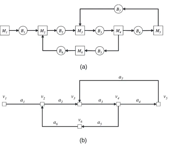
3-4 An assembly/disassembly network and its underlying digraph. (a) A 6-machine 7-buffer assembly/disassembly network. (b) The underlying
digraph . . . 66
4-1 Domains and ranges of blocking and starvation . . . 83
4-2 A five-machine production line . . . 84
4-3 A tree-structured network . . . 86
4-4 A single-loop system, Ω1 . . . 87
4-5 A system with two coupled loops, Ω2 . . . 89
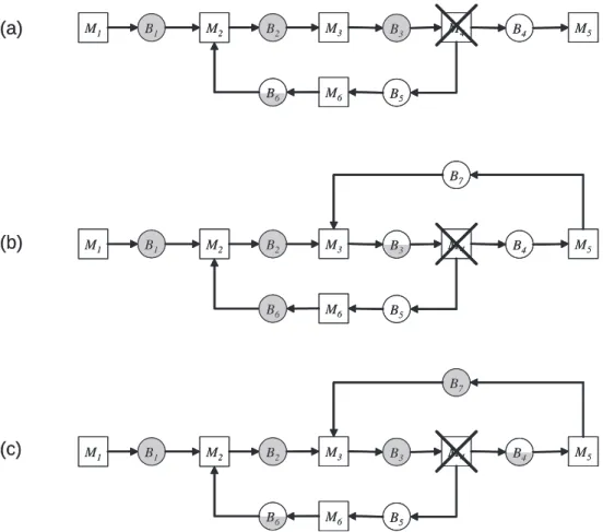
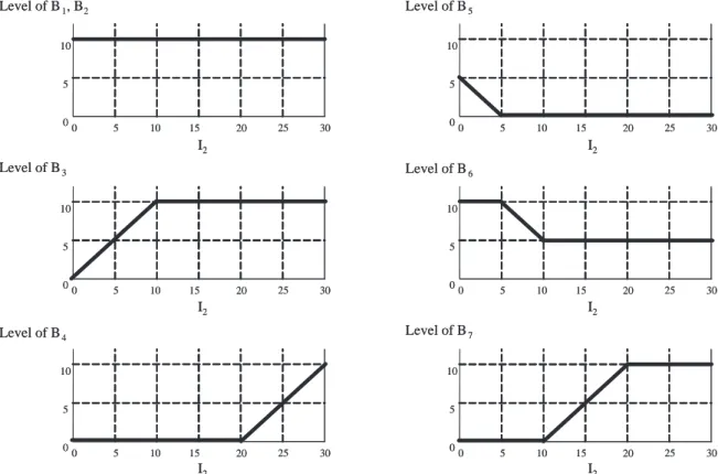
4-6 Buffer levels in the limiting propagation state due to the single machine failure at M3. (a) Single-loop system Ω1. (b) Two-loop system Ω2 (I2 = 15). (c) Two-loop system Ω2 (I2 = 25). . . 91
4-7 Buffer levels in the limiting propagation state due to a single machine failure at M3 . . . 92
4-8 Buffer levels in the limiting propagation state due to the single machine failure at M4. (a) Single-loop system Ω1. (b) Two-loop system Ω2 (I2 = 5). (c) Two-loop system Ω2 (I2 = 25). . . 94
4-9 Buffer levels in the limiting propagation state due to a single machine failure at M4 . . . 95
4-10 A spanning tree and a set of chords of a digraph G. (a) Digraph G. (b) Spanning tree T and the set of chords of T . (c) Set of fundamental circuits of G with respect to T . (Chords are indicated by dashed lines.) 97 4-11 Selection of a spanning tree. (a) A Two-loop system Ω. (b) A set of fundamental loops L of Ω. (c) A valid spanning tree T with respect to L. (d) An invalid spanning tree T with respect to L. . . 100
4-12 Induction sequence of a four-loop network . . . 102
4-13 Overflow and overdraft . . . 109
4-14 Subsystems of a two-loop system. (a) Ω0: tree-structured network. (b) Ω1: single-loop system. (c) Ω2: two-loop system. . . 114
5-2 Threshold in a buffer . . . 122
5-3 System transformation. (a) Divide the buffer into sub-buffers. (b) Two-machine one-buffer component after transformation. . . 123
5-4 Transformation of a two-loop system. . . 125
5-5 Routing buffer of failure propagation . . . 129
5-6 Remote failure mode λu ih(j) of the upstream pseudo-machine of BB(j) 137 5-7 Remote failure mode λd ih(j) of the downstream pseudo-machine of BB(j)139 6-1 An example of network equivalence . . . 157
7-1 Experiment architecture . . . 166
7-2 The percent errors of production rate of 1500 cases . . . 168
7-3 The distribution of the percent errors of production rate . . . 168
7-4 The absolute percent errors of production rate of 1500 cases . . . 169
7-5 The distribution of the absolute percent errors of production rate . . 169
7-6 The average percent errors of buffer levels of 1500 cases . . . 170
7-7 The average absolute percent errors of buffer levels of 1500 cases . . . 170
7-8 The average percent errors of loop invariants of 1500 cases . . . 171
7-9 The average absolute percent errors of loop invariants of 1500 cases . 171 7-10 The absolute percent errors of production rate VS Network scale . . . 173
7-11 The absolute percent errors of production rate VS Number of loops . 174 7-12 The computation time VS Network scale . . . 174
8-1 A five-machine CONWIP-controlled production line . . . 178
8-2 Comparison of three control options . . . 179
8-3 Production rate and total inventory level vs. Loop invariant (identical machines) . . . 181
8-4 Production rate and total inventory level vs. Loop invariant (noniden-tical machines) . . . 182
8-5 Control curve: production rate vs. total inventory level (nonidentical machines) . . . 183
8-6 A 5-machine production line and five variations of control structures . 185 8-7 Comparison of the total inventory levels of five control structures . . 186 8-8 Crossing between control curves due to infection points . . . 188 8-9 Comparison of the profits of five control structures (CP = 1000, CT = 1)190
8-10 Comparison of the profits of five control structures (CP = 1000, CT = 2)190
8-11 Comparison of the profits of five control structures (CP = 1000, CT = 10)191
8-12 Control curves and objective coefficient vectors . . . 192 8-13 Comparison of the inventory holding costs of five control structures
(Cost scheme #1) . . . 194 8-14 Comparison of the inventory holding costs of five control structures
(Cost scheme #2) . . . 195 8-15 Comparison of the inventory holding costs of five control structures
(Cost scheme #3) . . . 195 8-16 Comparison of the inventory holding costs of five control structures
(Cost scheme #4) . . . 196 8-17 Comparison of the inventory holding costs of five control structures
(Cost scheme #5) . . . 196 8-18 Comparison of the inventory holding costs of five control structures
(Cost scheme #6) . . . 197 8-19 Comparison of inventory distributions (production rate = 0.793) . . . 198 8-20 A double-loop control of a 5-machine production line . . . 200 8-21 Production rate plot of a double-loop control structure . . . 201 8-22 Total inventory level plot of a double-loop control structure . . . 201 8-23 Determine the optimal loop invariants of a double-loop control . . . . 202 8-24 Comparison of the total inventory levels of double-loop control and
single-loop control . . . 203 8-25 A 10-machine production line with bottleneck and five variations of
closed loop control . . . 208 8-26 Comparison of the total inventory levels of single-loop control structures209
8-27 Comparison of the total inventory levels of two single-loop control structures and a double-loop control structure . . . 209 8-28 Comparison of inventory distributions (production rate = 0.662) . . . 211 8-29 An assembly system with two sub-lines and three variations of closed
loop control . . . 213 8-30 Comparison of the total inventory levels of three control structures . . 217 8-31 Comparison of the total inventory holding costs of Structure # 3 while
varying I2 (cost scheme #1) . . . 218
8-32 Comparison of the total inventory holding costs of Structure # 3 while varying I2 (cost scheme #2) . . . 219
8-33 Comparison of the total inventory holding costs of Structure # 3 while varying I2 (cost scheme #3) . . . 219
8-34 An assembly system with nonidentical sub-lines . . . 221 8-35 Determine the optimal loop invariants of an assembly system with
identical sub-lines controlled by Structure #1 . . . 222 8-36 Determine the optimal loop invariants of an assembly system with
nonidentical sub-lines controlled by Structure #1 . . . 222 8-37 Three combination of different production rates and cost schemes of
an assembly system . . . 224 8-38 Determine the optimal loop invariants of an assembly system with
nonidentical sub-lines controlled by Structure #1 (cost scheme #1) . 224 8-39 Determine the optimal loop invariants of an assembly system with
nonidentical sub-lines controlled by Structure #1 (cost scheme #2) . 225 8-40 Determine the optimal loop invariants of an assembly system with
nonidentical sub-lines controlled by Structure #1 (cost scheme #3) . 226 A-1 Machine Mg and its upstream and downstream buffers and machines 256
B-1 A 15-machine 4-loop assembly/disassembly network . . . 261 B-2 An 18-machine 8-loop assembly/disassembly network . . . 264 B-3 A 20-machine 10-loop assembly/disassembly network . . . 266
List of Tables
1.1 Design parameters and performance measures of a CONWIP-controlled production line . . . 31 1.2 Profits of five cases in six scenarios . . . 32 6.1 Comparison of performance of equivalent networks (deterministic
process-ing time model) . . . 158 6.2 Comparison of performance of equivalent networks (continuous
mate-rial model) . . . 159 7.1 Comparison of computation time of ADN algorithm and simulation . 175 8.1 Comparison of three control options (target production rate = 0.7) . 179 8.2 Comparison of five control structures (target production rate = 0.825) 186 8.3 Six cost schemes of a production line . . . 193 8.4 Three cost schemes of an assembly system . . . 217 8.5 Three combinations of different production rates and cost schemes of
Chapter 1
Introduction
1.1
Motivation
1.1.1
Summary of Kanban Systems
Kanban means card or token. A kanban-controlled production system is one where
the flow of material is controlled by the presence or absence of a kanban, and where kanbans travel in the system according to certain rules.
The study of kanban-controlled systems can be traced back to the Toyota Pro-duction System in the 1950s. The classic kanban-controlled system was designed to realize Just-In-Time (JIT) production, keeping a tight control over the levels of individual buffers, while providing a satisfactory production rate (Figure 1-1).
5 2 6 3 7 4 1 Kanban attach Machine Material buffer (infinite)
Material flow Kanban flow Kanban detach
Kanban buffer (infinite)
5 2 6 3 7 4 1 5 2 6 3 7 4 1 Kanban attach Machine Material buffer (infinite)
Material flow Kanban flow Kanban detach
Kanban buffer (infinite)
Kanban attach Machine Material buffer (infinite)
Material flow Kanban flow Kanban detach
Kanban buffer (infinite)
From the perspective of control, feedback is implemented at each processing stage by circulating kanbans from its downstream buffer to the upstream of the stage. The circulation routes of kanbans form one closed loop per stage. Each stage has one control parameter: the number of kanbans. In the classic kanban-controlled system, a constant number of kanbans is imposed to limit the level of the buffer inventory in each closed loop. An infinite buffer controlled by a closed loop is equivalent to a finite buffer since the maximal inventory level can have in the infinite buffer is limited by the number of kanbans. The size of the finite buffer is equal to the number of kanbans in the loop.
There are several variations of kanban control widely used in industry, such as CONWIP control and hybrid control (Figure 1-2). Unlike the classic kanban-controlled system which uses kanbans to regulate the levels of individual buffers, the other two systems in Figure 1-2 implement a control strategy which limits the sum of the buffer levels within the large closed loop. Feedback is implemented from the last stage to the first stage.
(a) 1 5 2 3 4 (b) 4 1 5 2 3 6 Kanban attach Machine Material buffer (infinite)
Material flow Kanban flow Kanban detach
Kanban buffer (infinite) (a) 1 5 2 3 4 (b) 4 1 5 2 3 6 Kanban attach Machine Material buffer (infinite)
Material flow Kanban flow Kanban detach
Kanban buffer (infinite) Kanban attach
Machine Material buffer (infinite)
Material flow Kanban flow Kanban detach
Kanban buffer (infinite)
Figure 1-2: Variations of kanban systems
(a) CONWIP-controlled system; (b) Hybrid-controlled system
are separate operations before the work pieces proceed to machine operations. Notice that the operations of detaching and attaching kanbans are instantaneous compared to machine operations. Therefore, we integrate the kanban detach, kanban attach, and machine operation as one single operation (Figure 1-3). In addition, when kanbans are attached to workpieces, an integrated flow is used to represent two separate kanban and material flows in Figure 1-1 and Figure 1-2. In the remainder of this thesis, we use rectangles to represent integrated operations, and arrows to represent integrated flows.
Integrated operation
Integrated flow
Kanban attach
Machine Kanban detach Material flow Kanban flow Integrated flow
Integrated operation
Integrated flow
Kanban attach
Machine Kanban detach Kanban attach Material flow Kanban flow Integrated flow Machine Kanban detach Material flow Kanban flow Integrated flow
Figure 1-3: Integrated operation including kanban detach, kanban attach, and ma-chine operation
1.1.2
Essence of Kanban Control
Consider the system in Figure 1-1. Once a part enters a closed loop, a kanban card is attached to it. The kanban card is detached from the part when it leaves the closed loop and proceeds to the next stage. The number of kanbans within the closed loop is constant. We define it as the invariant of the loop. Similarly, when we look at the CONWIP loop in Figure 1-2(a), kanban cards are attached to the parts at the first stage of the production line while they are detached from the parts at the last stage. The total number of kanbans circulated within the CONWIP loop gives the loop invariant I:
I = b(1, t) + b(2, t) + b(3, t) + b(4, t) + b(5, t) (1.1) in which b(i, t) is the level of buffer Bi at time t.
The invariant imposes an upper limit of the buffer levels within the closed loop. For example, the total number of parts W allowed in the large CONWIP loop is constrained by:
W = b(1, t) + b(2, t) + b(3, t) + b(4, t) ≤ I (1.2) More generally, systems using kanban controls can be represented as a set of systems with multiple-loop structures. Each closed loop has a loop invariant. In the remainder of this thesis, material and kanban buffers are assumed to be finite because it is impossible to have infinite buffers in real world. A finite buffer is equivalent to an infinite buffer controlled by a classic kanban loop.
1.1.3
Importance of Multiple-Loop Structures
To control a given production system, a variety of kanban control methods can be used. Classic kanban control, CONWIP control and hybrid control are compared by Bonvik (1996), Bonvik et al. (1997), and Bonvik et al. (2000). The hybrid control method is demonstrated to have the best inventory control performance among these three control methods. Therefore, to study the design of control structures is valuable for developing insights into operational control.
After we determine the control structure, the design parameters of the closed loop, such as the number of kanbans, are also related to the system’s performance and cost. Consider a production line with pallets in Figure 1-4. CONWIP control is implemented by circulating pallets instead of kanban cards. Raw parts are loaded on pallets at machine M1 and unloaded from pallets at machine M10.
In the system, all machines are identical with failure rate p = 0.01, repair rate
r = 0.1, and processing rate µ = 1.0. All the material buffer sizes are 20. We
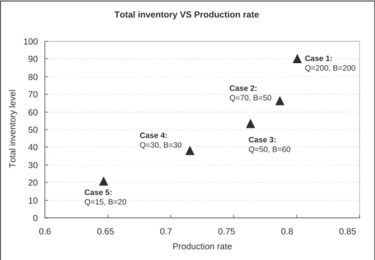
vary the number of pallets Q and the size of pallet buffer B to generate five cases. The parameters and performance measures in terms of production rate and total inventory level are summarized in Table 1.1. The performance measures are plotted in Figure 1-5.
Machine Material buffer Pallet buffer Material flow Pallet flow
1 1 2 2 3 …… 8 8 9 9 10
10
Machine Material buffer Pallet buffer Material flow Pallet flow
1 1 2 2 3 …… 8 8 9 9 10
10
Figure 1-4: CONWIP control of a production line with pallets
Case Number Q B Production rate P Total inventory level Tinv
1 200 200 0.800288 90.1366
2 50 70 0.786535 66.41147
3 60 50 0.763461 53.30389
4 30 30 0.715328 38.18662
5 20 15 0.646548 20.80521
Table 1.1: Design parameters and performance measures of a CONWIP-controlled production line
Total inventory VS Production rate
0 10 20 30 40 50 60 70 80 90 100 0.6 0.65 0.7 0.75 0.8 0.85 Production rate T o ta l in ve n to ry le ve l Case 1: Q=200, B=200 Case 3: Q=50, B=60 Case 2: Q=70, B=50 Case 4: Q=30, B=30 Case 5: Q=15, B=20
Total inventory VS Production rate
0 10 20 30 40 50 60 70 80 90 100 0.6 0.65 0.7 0.75 0.8 0.85 Production rate T o ta l in ve n to ry le ve l Case 1: Q=200, B=200 Case 3: Q=50, B=60 Case 2: Q=70, B=50 Case 4: Q=30, B=30 Case 5: Q=15, B=20
Figure 1-5: Production rate and total inventory level of CONWIP control while varying number of pallets Q and size of pallet buffer B
As these pallets cost money and take up space, the optimal selection of design parameters, such as the number of pallets and the storage buffer space of the pallets, has a significant dollar impact in profit. We formulate the profit Y as a function of production rate P , total inventory level Tinv, number of pallets Q, and size of pallet
buffer B:
Y = CPP − CTTinv− CQQ − CBB (1.3)
where CP is margin per unit production rate; CT, CQ, and CB are cost coefficients
of inventory, pallet, and pallet buffer, respectively.
We perform a set of scenario analyses by varying the margin and cost coefficients. The profits of five cases in six scenarios are listed in Table 1.2. We observe that, when pallet cost or pallet buffer cost is high (Scenarios 3 or 6), the optimal solution is Case 5, which has the smallest number of pallets and smallest pallet buffer.
Scenario Coefficients Profit of 5 cases Optimal Number CP CT CQ CB Case 1 Case 2 Case 3 Case 4 Case 5 Case
1 1000 1 0 1 510.15 650.12 660.16 647.14 610.74 3 2 1000 1 0 2 310.15 580.12 610.16 617.14 595.74 4 3 1000 1 0 10 -1289.85 20.12 210.16 377.14 475.74 5 4 1000 1 1 1 310.15 600.12 600.16 617.14 590.74 4 5 1000 1 2 1 110.15 550.12 540.16 587.14 570.74 4 6 1000 1 10 1 -1489.85 150.12 60.16 347.14 410.74 5
Table 1.2: Profits of five cases in six scenarios
In summary, the performance and cost of multiple-kanban production systems depend not only on control structures, but also on parameters such as number of kanbans. Therefore, an exhaustive study of the behavior of multiple-loop structures is needed. This study is challenging but highly valuable. It will provide a theoret-ical basis and practtheoret-ical guidelines for factory design and operational control using multiple-loop structures.
1.2
Background and Previous Work
In recent years there has been a large amount of literature on the analysis and design of kanban systems. The methods can be categorized into simulation and analytical methods. As the analysis and design of kanban systems usually involve evaluat-ing a large number of variations with different structures and parameters, analytical methods are much more promising in terms of computational efficiency. Another ad-vantage of analytical methods is their effectiveness in investigating the properties of multiple-loop structures and developing intuition for system design and control.
In this section, we review the development of manufacturing systems engineering with focus on the analytical work. Key issues and difficulties in analyzing systems with multiple-loop structures are explained. The review helps further understand the motivation of this research.
1.2.1
Fundamental Models and Techniques
A large number of models and methods have been developed to address the design and operations of manufacturing systems. An extensive survey of the literature of manu-facturing systems engineering models up to 1991 appeared in Dallery and Gershwin (1992). More recent surveys can be found in Gershwin (1994), Altiok (1997), and Hel-ber (1999). A review focused on MIT work and closely related research was presented by Gershwin (2003).
Initially, the research of this area started from modeling two-machine transfer lines with unreliable machines and finite buffers using Markov chains (Buzacott and Shanthikumar 1993). When Markov chains are used to model the stochastic behavior inherent in larger manufacturing systems, the scale and complexity of these systems often result in a huge state space and a large number of transition equations.
Decomposition was invented as an approximation technique to evaluate complex manufacturing systems by breaking them down into a set of two-machine lines (build-ing blocks). These build(build-ing blocks can be evaluated analytically by us(build-ing methods in Gershwin (1994). Gershwin (1987) was one of the first authors to analyze
finite-buffer production lines by developing an approximate decomposition method. Mascolo et al. (1991) and Gershwin (1991) extended the decomposition method to analyze tree structured assembly/disassembly networks.
Consider the decomposition of a long production line in Figure 1-6. Each buffer in the original system has a corresponding two-machine line (building block). The buffer of this building block has the same size as the original buffer. In each building block, its upstream and downstream machines are pseudo-machines which approximate the behavior observed in the original buffer. Each pseudo-machine is assigned one failure mode. The building blocks are evaluated iteratively and the failure rate and repair rate of each failure mode are updated till convergence.
Downstream pseudo-machine Upstream pseudo-machine …… …… …… …… Downstream pseudo-machine Upstream pseudo-machine …… …… …… ……
Figure 1-6: Long production line decomposition
1.2.2
Decomposition Using Multiple-Failure-Mode Model
A new decomposition method was presented by Tolio and Matta (1998). This method models the two-machine lines (building blocks) by assigning multiple failure modes to the pseudo-machines, instead of using single failure mode for each pseudo-machine.
In this model, the downstream pseudo-machine is assigned all the failure modes in the original system that can cause the original buffer to be full. The failure modes in the original system that can cause the original buffer to be empty belong to the upstream pseudo-machine.
For example, the decomposition of a six-machine production line using Tolio’s multiple-failure-mode model is shown in Figure 1-7. When the tandem line is de-composed into a set of building blocks, the building block corresponding to buffer B2
approximates the behavior observed by a local observer at B2. The failure modes of
machines M1 and M2 are assigned to the upstream pseudo-machine Mu(2) as they can
cause B2 to be empty; while the failure modes of M3, M4, M5, and M6 are assigned
to the downstream pseudo machine Md(2) as they can cause B
2 to be full. 4 3 2 2 3 4 5 1 1 5 6 Downstream pseudo-machine Upstream pseudo-machine Mu(2) 2 Md(2) Up Down(1) Down(3) p(1) r(1) r(3) Down(2) p(2) r(2) p(3) Up Down(6) Down(4) p(6) r(6) p(4) Down(5) p(5) r(5) r(4) 4 3 2 2 3 4 5 1 1 5 6 Downstream pseudo-machine Upstream pseudo-machine Mu(2) 2 Md(2) Up Down(1) Down(3) p(1) r(1) r(3) Down(2) p(2) r(2) p(3) Up Down(6) Down(4) p(6) r(6) p(4) Down(5) p(5) r(5) r(4)
Figure 1-7: Decompose a six-machine production line using multiple-failure-mode model
Up to this point, the systems we discussed are acyclic systems. In other words, there is no closed loop in these systems.
1.2.3
Systems with Closed Loops
In the studies of systems with closed loops, Frein et al. (1996), Werner (2001) and Gersh-win and Werner (2006) developed an efficient method to evaluate large single-loop systems using the decomposition method based on multiple-failure-mode model. Lev-antesi (2001) extended it to evaluate small multiple-loop systems. However, this method is not able to provide satisfactory speed and reliability while evaluating large-scale multiple-loop systems. Levantesi’s method demonstrated the feasibility
of his approach. But it had a very inefficient method for analyzing the propagation of blocking and starvation.
In addition, a systematic understanding of the behavior of multiple-loop struc-tures has not been developed yet. It is important as we need it for developing meth-ods for optimal design and control using multiple closed loops. Key issues include how to choose control structures, and determine kanban quantities. In the litera-ture, Monden (1983) presents the Toyota approach for determining the number of kanbans for each stage. This method, however, does not fully consider the random-ness due to machine failures and depends on subjective parameters, such as safety factor. Several methods are presented in Hopp and Spearman (1996), Hopp and Roof (1998), Ryan et al. (2000), and Ryan and Choobineh (2003) to determine WIP level for CONWIP-controlled systems. These methods have the disadvantages that the manufacturing systems for control are simple production lines, and the methods are limited to specified control structure — CONWIP. There are some studies on the variations of kanban control stuctures in Gaury et al. (2000, 2001). However, these approaches are simulation-based and the number of variations is limited.
In summary, the studies in the literature have the following two limitations:
• The manufacturing systems for control have relatively simple structures, such
as production lines or simple assembly systems. In fact, manufacturing systems are much more complicated in real factories.
• The control structures used are classic methods, such as single-stage kanban,
CONWIP. Multiple-loop control structures might have better performance than the classic ones.
One of the reasons for these limitations is that there are no efficient methods for evaluating complex manufacturing systems with multiple-loop structures. Therefore, an efficient evaluation method is desired such that the behavior of multiple-loop control can be explored to help design and control complex manufacturing systems.
1.3
Research Goal and Contributions
This thesis is intended to investigate the behavior of multiple-loop structures, to develop mathematical models and efficient analytical methods to evaluate system performance, and to help design factories. Specifically, the contributions of this thesis include:
• A unified assmebly/disassembly network model to represent multiple-loop
struc-tures which integrates information flows with material flows. (Refer to Chapter 2.)
• A systematic method to analyze blocking and starvation propagation based on
graph theory. (Refer to Chapters 3 and 4.)
• An efficient algorithm to evaluate large-scale assembly/disassembly systems
with arbitrary topologies. (Refer to Chapters 5 and 6.)
• Numerical experiments that demonstrate the algorithm is accurate, reliable,
and fast. (Refer to Chapter 7.)
• Characteristic behavior analysis of systems with multiple-loop structures.
(Re-fer to Chapter 8.)
• Insights for optimal design and control of production lines and assembly
sys-tems. (Refer to Chapter 8.)
• Practical guidelines for the design and operational control of multiple-kanban
production systems. (Refer to Chapter 8.)
1.4
Thesis Outline
We introduce assembly/disassembly networks with multiple-loop structures in Chap-ter 2. This model is used to integrate information flows with maChap-terial flows. To analyze the machine failure and blocking and starvation propagation in systems with
complex topologies, in Chapter 3, we develop a graph model. In Chapter 4, the analysis of blocking and starvation is discussed based on the graph model. The de-composition method is provided in Chapter 5. In Chapter 6, we present an efficient algorithm for evaluating assembly/disassembly networks with arbitrary topologies. Chapter 7 discusses the performance of the algorithm in terms of accuracy, reliability and speed. In Chapters 8, we present the behavior analysis and design insights on production control using multiple-loop structures. Finally, a summary of the con-tributions of this research, and a brief description of future research directions are presented in a conclusion in Chapter 9.
Chapter 2
Assembly/Disassembly Networks
with Multiple-Loop Structures
A set of production control policies using multiple closed-loop structures, such as clas-sic kanban, CONWIP, hybrid control, have been invented and implemented. Kanban cards perform as media which convey information flows to control material flows. In this chapter, we develop a model to provide an integrated view of material flows and information flows.
First, in Section 2.1, assembly/disassembly networks with multiple-loop structures are presented as a unified model to integrate information flows with material flows. Two important properties — assembly/disassembly operations, and loop invariants — are discussed. In Section 2.2, we present an approach to evaluating system perfor-mance. The challenges in evaluation are discussed in Section 2.3.
2.1
A Unified Model
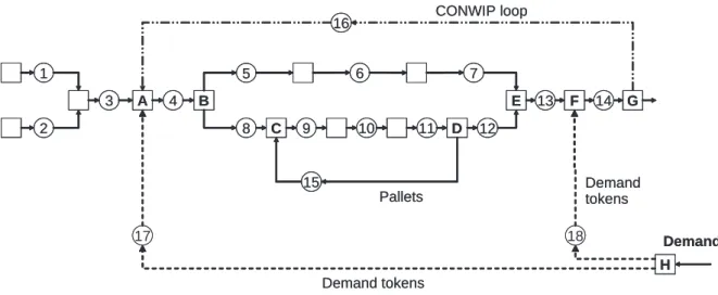
Consider the system in Figure 2-1. The machines in the system are only allowed to perform single part, assembly, or disassembly operations. (We do not include merges or splits of flows.) Material flow is disassembled into two sub-flows at machine MB
and these two sub-flows are reassembled at machine ME. The processes in the lower
CONWIP control loop is implemented between machine MGand MA. Demand tokens
are generated by machine MH for base stock control at machines MA and MF. Four
closed loops are formed in the system.
A B C 4 5 9 F 13 E 6 D 12 G 14 15 16 7 8 2 1 3 10 11 H Demand Demand tokens CONWIP loop Demand tokens Pallets 17 18 A B C 4 5 9 F 13 E 6 D 12 G 14 15 16 7 8 2 1 3 10 11 H Demand Demand tokens CONWIP loop Demand tokens Pallets 17 18
Figure 2-1: An assembly/disassembly network with four closed loops
Four loops can be identified in the network:
• Loop 1: B5 → B6 → B7 → B12 → B11→ B10→ B9 → B8;
• Loop 2: B9 → B10→ B11 → B15;
• Loop 3: B4 → B8 → B9 → B10 → B11→ B12→ B13 → B14→ B16;
• Loop 4: B4 → B8 → B9 → B10 → B11→ B12→ B13 → B18→ B17.
2.1.1
Assembly/Disassembly Operations
Traditionally, assembly/disassembly is used to describe a process involving two or more real workpieces. However, this need not to be the case. Various meanings of assembly/disassembly operations are represented in the unified graph of Figure 2-1.
Sometimes, a workpiece is assembled to a pallet or fixture when it enters a system. After going though a set of processes, the workpiece is disassembled from the pallet. Therefore, assembly/disassembly takes place between a real workpiece and a fixture or pallet. For example, machines MB and ME in Figure 2-1 perform disassembly and
assembly of real parts. Machines MC and MD disassemble and assemble real parts
with pallets.
When we consider kanban control, the attach and detach operations between kanbans and workpieces are actually assembly/disassembly operations. By imagining the kanban as a medium which conveys control information, the assembly/disassembly operations take place between information flows and material flows. For example, at machine MG, kanbans are disassembled from real workpieces; while at machine MA,
kanbans are assembled with real workpieces. The kanbans take the information from downstream machine MG to upstream machine MA such that new workpieces are
authorized to be dispatched from buffer B3.
More interestingly, Gershwin (2000) shows that the demand information can be embedded into a production line with material flow by using virtual assembly/disassembly machines. In Figure 2-1, machine MH is a demand machine which generates demand
token flows by disassembly. The demand tokens are assembled with real parts at machines MA and MF. The stock level between MA and MF is controlled.
Assembly/disassembly machines in assembly/disassembly networks have the fol-lowing property:
Equality of Flows When an assembly/disassembly machine completes one oper-ation, each of its upstream buffers is decreased by one workpiece, while each of its downstream buffers is increased by one workpiece. In any given time frame, the amount of material coming from each upstream buffer of an assembly/disassembly machine is equal to the amount of material going into each downstream buffer of the machine.
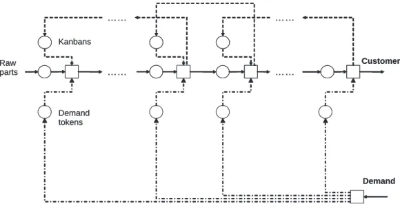
Here we illustrate one example of the Extended Kanban Control Systems (EKCS) described in Dallery and Liberopoulos (2000). The EKCS is modeled as an assem-bly/disassembly network in Figure 2-2. Kanbans are circulated between machines and demand tokens are used to implement base stock control. A machine in the system could assemble kanbans (e.g. demand tokens) with real workpieces, and disassemble
Demand Kanbans Demand tokens …… …… …… …… Customer Raw parts Demand Kanbans Demand tokens …… …… …… …… Customer Raw parts
Figure 2-2: An extended kanban control system (EKCS)
kanbans from real workpieces.
2.1.2
Loop Invariants
In Chapter 1, we briefly introduce the loop invariant by illustrating a CONWIP loop example. Here, we provide a general definition of a loop invariant.
In Figure 2-3(a), the total number of workpieces travelling in the closed loop is a constant of time. The constant number of workpieces is the loop invariant:
I = b(1, t) + b(2, t) + b(3, t) + b(4, t) (2.1)
in which b(i, t), i = 1, ..., 4 are the buffer levels of Bi, i = 1, ..., 4 at time t.
In the above loop, the flow follows a single direction. In other words, there is no direction change within the closed loop and the flow is unidirectional. When the flow in the closed loop is not unidirectional, we can also define the invariant but in a more complex way.
Consider the variation of single loop in Figure 2-3(b), which has flow direc-tion changes at M1 and M3. Although there is no part circulated in this
Invariant M2 B1 M1 B4 M3 B2 M4 B3 B1 M2 M1 B3 B2 B4 M4 M3
(a)
(b)
M2 B1 M1 B4 B2 B5 M5 M3 M4 B3 M6 B6(c)
Invariant= b(1,t) + b(2,t) + b(3,t) + b(4,t) Invariant= b(1,t) + b(2,t) -b(3,t) -b(4,t) Invariant = b(1,t) + b(2,t) -b(3,t) + b(4,t) + b(5,t) -b(6,t) Invariant Invariant Invariant M2 B1 M1 B4 M3 B2 M4 B3 B1 M2 M1 B3 B2 B4 M4 M3(a)
(b)
M2 B1 M1 B4 B2 B5 M5 M3 M4 B3 M6 B6(c)
Invariant= b(1,t) + b(2,t) + b(3,t) + b(4,t) Invariant= b(1,t) + b(2,t) -b(3,t) -b(4,t) Invariant = b(1,t) + b(2,t) -b(3,t) + b(4,t) + b(5,t) -b(6,t) Invariant Invariantmachine M1. According to the property of ‘equality of flows’, whenever one sub-part
goes into the upper branch, there must be the other sub-part going into the lower branch. Similar things happen to the assembly at machine M3. Therefore, the
differ-ence between the sum of the buffer levels of the upper branch and that of the lower branch is a constant of time. Usually, the constant is zero in disassembly/reassembly systems. However, it can be non-zero value which depends on the initial condition of the distribution of buffer levels. For the loop in Figure 2-3(b), an invariant I can be expressed as follows:
I = b(1, t) + b(2, t) − b(3, t) − b(4, t) (2.2)
A more complicated variation of a single loop is shown in Figure 2-3(c). The flow direction changes four times in the loop. Loop orientation, as an abstract concept, is introduced for the purpose of defining the invariant. An invariant can be then obtained by adding the levels of buffers whose direction agree with the loop orientation and subtracting the levels of all the rest. For example, assume the loop orientation is clockwise, the invariant of the loop in Figure 2-3(c) is given by
I = b(1, t) + b(2, t) − b(3, t) + b(4, t) + b(5, t) − b(6, t) (2.3) A general definition of loop invariant is summarized:
• Step 1: Define the loop orientation • Step 2: Given a buffer in the loop
– If the flow though the buffer agrees with the loop orientation, add the buffer level to the invariant.
– If the flow though the buffer does not agree with the loop orientation, subtract the buffer level from the invariant.
Incidentally, the number of direction changes in a closed loop is always an even number.
Recall the four loops in the assembly/disassembly network of Figure 2-1. Their loop invariants are defined as follows:
I1 = b(5, t) + b(6, t) + b(7, t) − b(12, t) − b(11, t) − b(10, t) − b(9, t) − b(8, t)
I2 = b(9, t) + b(10, t) + b(11, t) + b(15, t)
I3 = b(4, t) + (8, t) + b(9, t) + b(10, t) + b(11, t) + b(12, t) + b(13, t) + b(14, t) + b(16, t)
I4 = b(4, t) + b(8, t) + b(9, t) + b(10, t) + b(11, t) + b(12, t) + b(13, t) − b(18, t) + b(17, t)
(2.4) Loop invariants, as the basic property of closed loops, constrain the distribution of buffer levels and result in complicated behavior of blocking and starvation propa-gation. At this point, we only introduce the concept of loop invariants. Several key issues of the complicated behavior of blocking and starvation are discussed in Section 2.3. Detailed analysis is presented in Chapters 4 and 5.
In summary, assembly/disassembly networks are defined as a class of systems com-posed of finite buffers and unreliable machines which can perform single-stage oper-ation, assembly/disassembly, but NOT flow merge or split and NOT reentrant flow. The definition of assembly/disassembly operations is extended to include both mate-rial flows and information flows. Kanban, CONWIP, hybrid and other information-based control methods can be modeled as assembly/disassembly networks with multiple-loop structures.
2.2
Approach to Evaluation
Given an assembly/disassembly network with unreliable machines and finite buffers, we are interested to know the system performance in terms of production rate and average buffer levels. In this section, we presented an approach for evaluating assem-bly/disassembly networks with arbitrary topologies. The detailed procedures of this evaluation approach are presented in Section 6.2.
2.2.1
Decomposition
Markov chain processes are used to model stochastic behavior of machine failures and repairs in manufacturing systems. However, the state space is huge when sys-tem is large-scale. Decomposition has been developed as an approximation technique to evaluate large-scale complex manufacturing systems. Decomposition algorithms have been developed for production lines and tree-structured systems in Gershwin (1987), Mascolo et al. (1991), and Gershwin (1991). The multiple-failure-mode model developed by Tolio and Matta (1998) improves the efficiency of long line decomposi-tion, and enables the development of decomposition algorithms of closed-loop systems in Frein et al. (1996), Gershwin and Werner (2006) and Levantesi (2001).
All of the above decomposition techniques break down manufacturing systems into a set of two-machine one-buffer lines (building blocks), which can be evaluated analytically. For each buffer in the original system, a two-machine line is designed to approximate the behavior of flow observed in the buffer. The upstream pseudo-machine of the two-pseudo-machine line approximates the failures propagated from the up-stream portion of the system, while the downup-stream pseudo-machine approximates the failures propagated from downstream.
A rule for failure modes assignment is developed based on the multiple-failure-mode method in Tolio and Matta (1998):
Failure Modes Assignment Rule Given a building block corresponding to one buffer in the original system, failure modes in the original system which can cause the original buffer to be full are assigned to the downstream pseudo-machine; while the upstream pseudo-machine collects the failure modes in the original system which can cause the buffer to be empty.
When the original buffer is empty, its immediate downstream machine in the original system is starved. When the original buffer is full, its immediate upstream machine in the original system is blocked. Therefore, before we decompose the system into building blocks, we should first analyze the properties of blocking and starvation
propagation.
2.2.2
Blocking and Starvation Analysis
The phenomena of blocking and starvation result from the propagation of flow disrup-tion due to unreliable machines and finite buffers. For a given machine in the system, suppose one or more of its immediate downstream buffers is full. The machine is forced to stop processing parts. This situation is defined as blocking. Similarly, the situation of starvation is defined when the machine is forced to stop if one or more of its immediate upstream buffers is empty.
To obtain the blocking and starvation properties, we are interested to know the
‘Machine failure – Buffer level’ relationship in the limiting propagation state: given a
buffer, which machine failures in the system can cause the buffer to be full, and thus block the immediate upstream machines of the buffer? Which machine failures in the system can cause the buffer to be empty, and thus starve the immediate downstream machines of the buffer?
2.2.3
Summary of Evaluation Approach
We summarize the evaluation method for an assembly/disassembly network with arbitrary topology as follows:
• Phase I: Analyze blocking and starvation properties • Phase II: Decomposition
– Decompose the system into two-machine one-buffer building blocks; – Set up each building block according to blocking and starvation properties; – Iteratively evaluate building blocks using multiple-failure-mode model.
2.3
Challenges
When there is no closed loop in assembly/disassembly networks, the properties of blocking and starvation are straightforward and the decomposed building blocks can be easily set up (Gershwin 1991, 1994). However, when there exist closed loops, the invariants of these loops result in complicated blocking and starvation behavior.
2.3.1
Thresholds in Buffers
In systems without closed-loop structures, such as production lines or tree-structured systems, given a single machine failure which lasts for a sufficient amount of time and all other machines are operational, the buffer levels are eventually either full or empty. For systems with closed loops, loop invariants can cause some buffers to be partially filled.
Consider the unidirectional single loop in Figure 2-3(a). Suppose all buffer sizes are 10 and the loop invariant is 22. If M3 is failed for a sufficient amount of time and
all other machines are operational, the buffer levels in the limiting state are:
b(1, ∞) = 10; b(2, ∞) = 10; b(3, ∞) = 0; b(4, ∞) = 2;
so that the invariant is satisfied:
I = b(1, ∞) + b(2, ∞) + b(3, ∞) + b(4, ∞) = 22
B2 and B3 are full while B4 is empty. B1 is partially filled in order to satisfy the
invariant equation. The partially filled level is defined as a threshold in the buffer. According to the failure assignment rule described in Section 2.2, in a building block,
the failure modes of M3 can not be assigned to either upstream pseudo-machine or
downstream pseudo-machine. When we model building blocks using Markov chain processes, the methods developed in Gershwin (1994) and Tolio et al. (2002) can not be used because the transitions between the states in which the buffer level is above the threshold have different behavior than those between the states in which the buffer level is under the threshold. Therefore, a new method is needed to deal the thresholds in buffers. Maggio et al. (2006) presents a method for evaluating small loops with thresholds. A more efficient method for evaluating large loops is developed by Gershwin and Werner (2006). It eliminates thresholds by introducing perfectly reliable machines. This method is presented in Section 5.2.
To find the buffer levels in unidirectional loops is still simple. However, when there exist flow direction changes in loops, determining the buffer levels is much more complicated. Consider the single-loop system in Figure 2-3(c). The flow direction changes four times. Suppose the loop invariant is 28 and all buffer sizes are 10. If machine M3 goes down for a sufficient amount of time and all other machines are
operational, the buffer levels in the limiting state are:
b(1, ∞) = 10; b(2, ∞) = 10; b(3, ∞) = 10; b(4, ∞) = 8; b(5, ∞) = 10; b(6, ∞) = 0;
so that the invariant is satisfied:
I = b(1, ∞) + b(2, ∞) − b(3, ∞) + b(4, ∞) + b(5, ∞) − b(6, ∞) = 28
on the direction of flows. The buffer levels can not be easily determined unless the loop is carefully analyzed.
2.3.2
Coupling among Multiple Loops
When two loops have one or more common buffer, these two loops are coupled to-gether. Consider loop 1 and loop 3 in Figure 2-1.
• Loop 1: B5 → B6 → B7 → B12 → B11→ B10→ B9 → B8;
• Loop 3: B4 → B8 → B9 → B10 → B11→ B12→ B13 → B14→ B16;.
Loop 1 and loop 3 are coupled as they have common buffers B9, B10, and B11.
As there exist four loops in the system, all the buffer levels in the system should satisfy the invariant equations (2.4). Therefore, the distribution of buffer levels is constrained by the loop invariants and coupling structures.
2.3.3
Routing Buffer of Failure Propagation
In addition to the ‘Machine failure – Buffer level’ relationship described in Section 2.2.2, we need to know the routing buffer through which the machine failure is propa-gated. This information is essential for updating the parameters of pseudo-machines while performing iterative iterations during decomposition.
Consider the single loop system in Figure 2-4. All the buffer sizes are 10. The loop invariant is 5. For the building block corresponding to buffer B1, a single machine
failure at machine ME can cause B1 to be full. To satisfy the invariant condition, the
b(1, ∞) = 10; b(2, ∞) = 10; b(3, ∞) = 10; b(4, ∞) = 5; b(5, ∞) = 10;
such that the invariant is satisfied:
I = b(2, ∞) + b(3, ∞) − b(5, ∞) − b(4, ∞) = 5 (2.5)
There exist two paths which connect B1 and ME:
• Path 1: B1 → B2 → B3 → ME; • Path 2: B1 → B4 → B5 → ME; B C D E 2 4 3 5 A 1 Invariant = 5 1 Upstream pseudo-machine Failure modes: MA Downstream pseudo-machine Failure modes: MB, MC, MD, ME Path 1 Path 2 B C D E 2 4 3 5 A 1 Invariant = 5 1 1 Upstream pseudo-machine Failure modes: MA Downstream pseudo-machine Failure modes: MB, MC, MD, ME Path 1 Path 2
The failure at ME is propagated via Path 1 but not Path 2. Therefore, B2 is
de-fined as the routing buffer of the failure propagation from M4 to B1. The importance
and more details of routing buffers are presented in Section 5.3.2.
To summarize, in this section, several key issues are briefly discussed, including thresholds in buffers, coupling effects among multiple loops, and routing buffer of fail-ure propagation. These issues are very common in assembly/disassembly networks with complex multiple-loop structures. Given the complexity of blocking and starva-tion, efficient methods for analyzing blocking and starvation are desired. The detailed analysis and related methods are presented in Chapters 4 and 5. For the purpose of analyzing blocking and starvation of assembly/disassembly networks with complex multiple-loop structures, a graph model is developed in Chapter 3 as a framework for blocking and starvation analysis.
Chapter 3
Graph Model of
Assembly/Disassembly Networks
In the previous chapter, we define assembly/disassembly networks as a class of man-ufacturing systems composed of finite buffers and unreliable single-part or assem-bly/disassembly machines. The structure or topology of assemassem-bly/disassembly net-works can vary from a simple production line to a large-scale assembly/disassembly shop which contains over hundred machines and implements multiple kanban loops for production control.
In the literature (Dallery and Gershwin 1992, Buzacott and Shanthikumar 1993, Gershwin 1994, Altiok 1997), models of manufacturing systems are usually described by machine and buffer indices, and their upstream and downstream context. This rep-resentation scheme is sufficient to describe the systems with relatively simple topolo-gies. However, it becomes difficult to represent large-scale complex systems with multiple-loop structures using this way. When information flows are integrated with the material flows in the system to implement closed loop control, the complexity of the system topology is further increased. Therefore, a new method is required to efficiently represent manufacturing systems. From a graphical perspective, in any manufacturing system, machines and buffers are organized as a connected directed graph, i.e. a digraph. Graph theory, therefore, is introduced as a generic framework to represent assembly/disassembly networks.
This chapter presents, in the manufacturing system context, how to apply graph theory to develop a framework for the analysis and design of assembly/disassembly networks with arbitrary topologies. Section 3.1 introduces the graph theory basics which are directly related to the modeling of assembly/disassembly networks. The graph model is presented in Section 3.2. In Section 3.3, we discuss two important conditions of the graph model. Linear equation systems of connected flow networks are presented in Section 3.4. The notations introduced in this chapter are needed for the analysis in this thesis.
3.1
Graph Theory Basics
In this section, we introduce concepts in graph theory which are closely related to this thesis. The terminologies of graph theory vary from one book to another. The terminology used in this thesis is taken from Swamy (1981). For readers who are interested in further topics in graph theory and its applications, references can be found in Carre (1979), Swamy (1981), and Boffey (1982).
3.1.1
Some Essential Concepts
The central concept of a graph is that it is a set of entities called vertices or nodes, which are interrelated via certain correspondences called edges or links. A graph is often thought of as a set of points (representing vertices) with interconnecting lines (representing edges) and is frequently pictured in this way. Each edge is identified with a pair of vertices. If the edges of a graph are directed (with directions shown by arrows), in which case they are called arcs, then the graph is called a directed or an oriented graph. Otherwise, the graph is called an undirected graph. Since manufacturing systems are networks with directed flows, we restrict our discussions to directed graphs.
Digraphs, Vertices and Arcs
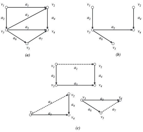
Formally, a directed graph or, for short, a digraph G = (V, A) consists of two sets: a finite set V of elements called vertices and a finite set A of elements called arcs. We use the symbols v1, v2, ... to represent the vertices and the symbols a1, a2, ... to
represent the arcs of a digraph. Some important concepts are:
• Each arc is associated with an ordered pair of vertices. If al = (vi, vj), then vi
and vj are called the end vertices of arc al. vi is the initial vertex while vj is
the terminal vertex of al.
• Two vertices are adjacent if they are the end vertices of the same arc.
• An arc is said to be incident on its end vertices. An arc is said to be incident out of its initial vertex and incident into its terminal vertex.
• An arc is called a self-loop at vertex vi, if vi is the initial as well as the terminal
vertex of the arc.
• The vertex set V can be decomposed into three subsets, X, Y and I. The
vertices in X are called sources, which only have outgoing arcs, while the vertices in Y are called sinks, which only have incoming arcs. Vertices in I, which are neither sources nor sinks, are called intermediate vertices.
In the pictorial representation of a digraph, a vertex is represented by a circle or rectangle and an arc is represented by an arrowhead line segment which is drawn from the initial to the terminal vertex.
For example, if
V = {v1, v2, v3, v3, v4, v5};
A = {a1, a2, a3, a4, a5, a6, a7};
a1 = (v1, v2); a2 = (v1, v3); a3 = (v3, v2); a4 = (v2, v4); a5 = (v3, v4); a6 = (v3, v5); a7 = (v5, v4).
then the digraph G = (V, A) is represented in Figure 3-1(a). In this digraph, v1 is a
source, v4 is a sink, and v2, v3, v5 are intermediate vertices.
v
1v
2v
3v
4v
5a
1a
2a
3a
4a
5a
6a
7v
1v
2v
3v
4v
5a
1a
2a
3a
4a
5a
6a
7 Figure 3-1: A digraphWalks, Trails, Paths, and Circuits
Here, we define the concepts of walks, trails, paths, and circuits. The directions of the arcs are not important in the definitions.
A walk in a digraph G = (V, A) is a finite alternating sequence of vertices and arcs v1, a1, v2, a2, ..., vk−1, ak−1, vk beginning and ending with vertices such that vi−1