Analyzing system performance with probabilistic performance annotations

(1)

Analyzing System Performance

with

Probabilistic Performance Annotations

Doctoral Dissertation submitted to the

Faculty of Informatics of the Università della Svizzera Italiana in partial fulfillment of the requirements for the degree of

Doctor of Philosophy

presented by

Daniele Rogora

under the supervision of

Prof. Antonio Carzaniga and Prof. Robert Soulé

(2)

(3)

Dissertation Committee

Prof. Matthias Hauswirth Università della Svizzera Italiana, Switzerland Prof. Fernando Pedone Università della Svizzera Italiana, Switzerland

Prof. Amer Diwan Google, Mountain View, USA

Prof. Timothy Roscoe ETH Zurich, Switzerland

Dissertation accepted on 11 January 2021

Research Advisor Co-Advisor

Prof. Antonio Carzaniga Prof. Robert Soulé

PhD Program Director

Prof. Walter Binder, Prof. Silvia Santini

(4)

I certify that except where due acknowledgement has been given, the work presented in this thesis is that of the author alone; the work has not been submit-ted previously, in whole or in part, to qualify for any other academic award; and the content of the thesis is the result of work which has been carried out since the official commencement date of the approved research program.

Daniele Rogora

Lugano, 11 January 2021

(5)

To Cecilia, may your journey know no limits

(6)

(7)

Abstract

Understanding the performance of software is complicated. For several perfor-mance metrics, in addition to the algorithmic complexity, one must also consider the dynamics of running a program within different combinations of hardware and software environments. Such dynamical aspects are not visible from the code alone, and any kind of static analysis falls short.

For example, in reality, the running time of asortmethod for a list is going

to be different from the expected O(n log n) complexity if the hardware does not have enough memory to hold the entire list.

Moreover, understanding software performance has become much more plex because software systems themselves continue to grow in size and com-plexity, and because modularity works quite well for functionality but less so for performance. In fact, the many subsystems and libraries that compose a modern software system usually guarantee well documented functional prop-erties but rarely guarantee or even document any performance behavior. Fur-thermore, while functional behaviors and problems can be reasonably isolated, performance problems are often interaction problems and they are pervasive.

Performance analysts typically rely on profilers to understand the behavior of software. However, traditional profilers like gprof produce aggregate informa-tion in which the essential details of input or context-specific behaviors simply get lost. Some previous attempts at creating more informative performance profiles require that the analyst provide the performance models for software compo-nents. Other performance modeling tools deduce those models automatically but consider only the abstract algorithmic complexity, and therefore fail to find or even express interesting runtime performance metrics.

In this thesis, we develop the concept of probabilistic performance annotations to understand, debug, and predict the performance of software. We also intro-duce Freud, a tool that creates performance annotations automatically for real world C/C++ software.

A performance annotation is a textual description of the expected perfor-mance of a software component. Perforperfor-mance is described as a function of

(8)

vi

tures of the input processed by the software, as well as features of the systems on which the software is running. Performance annotations are easy to read and un-derstand for the developer or performance analyst, thanks to the use of concrete performance metrics such as running time, measured in seconds, and concrete features, such as the real variables as defined in the source code of the program (e.g., the variable that stores the length of a list).

Freud produces performance annotations automatically using dynamic anal-ysis. In particular, Freud instruments a binary program written in C/C++ and collects information about performance metrics and features from the running program. Such information is then processed to derive probabilistic performance annotations. Freud computes regressions and clusters to create regression trees and mixture models that describe complex, multi-modal performance behaviors. We illustrate our approach to performance analysis and the use of Freud on three complex systems—the ownCloud distributed storage service; the MySQL database system; and the x264 video encoder library and application—producing non-trivial characterizations of their performance.

(9)

Acknowledgments

My sincere thanks go to my friendly advisor Antonio for his continuous guidance, teachings, and support.

I want to thank Alessandro, Gianpaolo, and Robert for guiding and encour-aging me in my academic career, and Ali, Koorosh, Michele, and Fang for sharing memorable steps during my path.

My dear friends Alberto, Cristina, Fabio, Grazia, Luca, Maria Elena, and Roberto for sharing joyful moments that helped in overcoming adversities.

My beloved family, my center of gravity, for their unlimited patience and un-conditional support.

Lastly, I want to thank those who think they do not deserve a spot here. Your friendship was an invaluable contribution in writing this thesis.

The achievement would have never been possible without the unique contri-bution of all these people. Thank you! Grazie!

(10)

(11)

Figures

1.1 Running time forstd::list<int>::sort . . . 5

1.2 Performance annotation for the running time oflist<int>::sort 7 1.3 Performance annotation for minor page faults forsort . . . 9

1.4 Performance annotation for major page faults forsort . . . 10

3.1 A performance annotation with regressions . . . 27

3.2 A performance annotation with regressions . . . 29

3.3 A performance annotation with clusters . . . 31

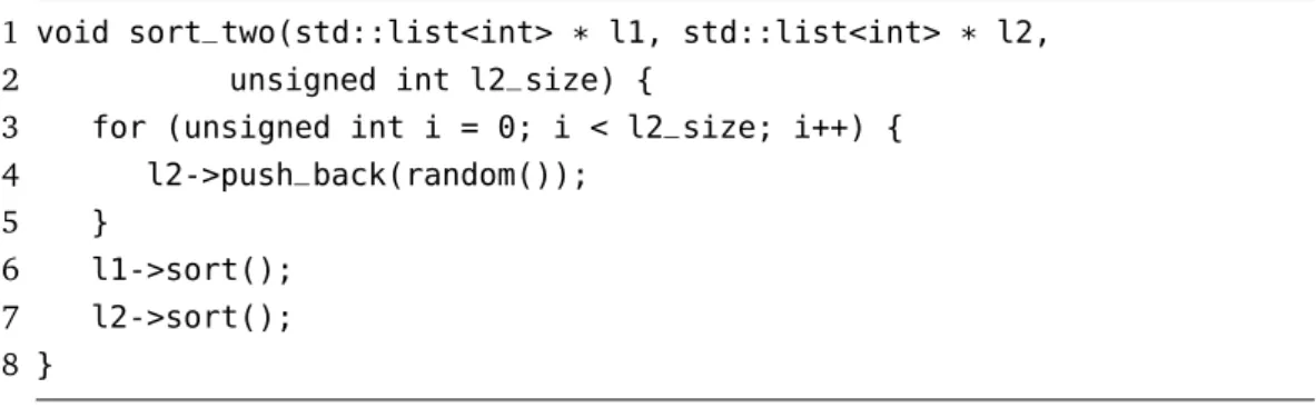
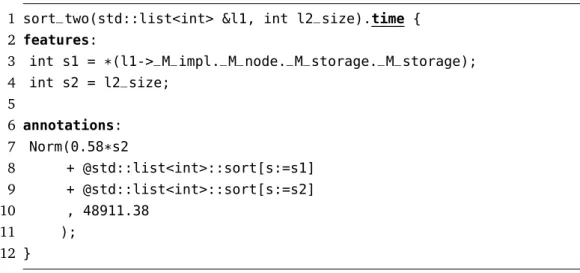
3.4 The C++ source code of sort_two . . . 32

3.5 A performance annotation without references . . . 32

3.6 A performance annotation with references . . . 33

3.7 A performance annotation with heuristics . . . 34

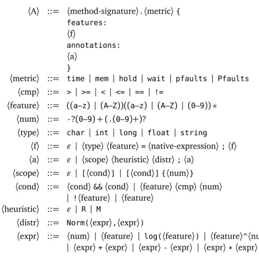
3.8 Grammar of the performance annotations language . . . 35

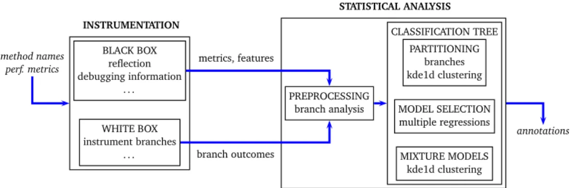
4.1 Overview of the derivation of performance annotations . . . 41

4.2 A classification tree with mixture models . . . 49

5.1 High-level architecture of Freud . . . 64

5.2 Example of DWARF tree for a C++ program . . . 67

5.3 Architecture of freud-dwarf . . . 72

5.4 Architecture of freud-pin . . . 79

5.5 Example of plots for regressions with interaction terms . . . 88

5.6 Runtime performance overhead of Freud . . . 92

6.1 ff_h2645_extract_rbsp: running time. . . 101

6.2 encoder_encode: running time without context switches. . . 102

6.3 encoder_encode: wait time seen from two different features . . . 104

6.4 slice_write, sliced vs. framed processing. . . 105

6.5 mysql_execute_command, 5.7.24 (top) vs. 8.0.11. . . 107

6.6 test_quick_select(): INvsAND/ORquery. . . 108

(16)

xiv Figures

6.7 get_func_mm_tree: arg_count feature . . . 109

6.8 Arithmetic progression ofkey_or(). . . 110

6.9 fseg_create_general: branch analysis. . . 111 6.10 Some annotations for ownCloud: linear and quadratic regressions

(top, middle) and clusters (bottom) . . . 113 6.11 Robustness, use of annotations to detect anomalies . . . 114

(17)

Tables

2.1 Comparison of different approaches to performance analysis . . . 22

3.1 Currently supported metrics and units of measurements . . . 27

5.1 Parameters and default values in freud-dwarf . . . 76

5.2 Parameters and default values in freud-pin . . . 85

5.3 Parameters and default values in freud-statistics . . . 89

5.4 Running time for freud-dwarf for three targets and different depths of feature exploration . . . 95

5.5 Statistics and performance (running time) of the statistical analy-sis for (a) themysql_execute_commandmethod of MySQL 5.7.24, (b) thex264_8_encoder_encodemethod of x264 with a sampling rate of 20 samples per second, and (c) thex264_8_encoder_encode method of x264 with a sampling rate of 50 samples per second. . 96

(18)

(19)

Chapter 1 Introduction

In this thesis we introduce a methodology for dynamic performance analysis for complex software systems. We also introduce a set of tools, Freud, that imple-ment such analysis. Freud creates probabilistic performance annotations for soft-ware components at different granularity, ranging from small utility methods to the main function of a program. These performance annotations describe cost functions that correlate some performance metrics measured on the running pro-gram with some features describing either the state of the propro-gram or the system on which the program is running.

The metrics are measurable quantities that describe the real behavior of the software system when running on real hardware. Example metrics are the run-ning time, measured in seconds, or the dynamic memory that is allocated, mea-sured in bytes. Other interesting metrics include lock holding or waiting time, or the number of memory page faults.

Similarly, the features are measurable values that describe the state of the program or of the system on which it is running. A feature may indicate the value of a variable, the number of threads being used by the program, or the clock frequency of the CPU.

One key aspect of the analysis is that it is almost completely automated. The performance analyst does not need a deep understanding of the system to gener-ate rich and meaningful performance annotations. Freud automatically finds the features that affect performance, and also manages to identify even non trivial, multi-modal performance behaviors.

Performance annotations created with Freud can serve as an intuitive doc-umentation of the performance of a system or as a performance specification. Additionally, the automatic generation of performance annotations can be trig-gered programmatically to accompany the development and evolution of a

(20)

2 1.1 Performance Analysis

ware system, similar to functional tests in continuous integration. In such a con-text or more generally, performance annotations can be used as assertions or test oracles, for example to detect performance regressions. Also, since they define cost functions, performance annotations can extrapolate what is measured ex-perimentally to predict the performance of a software system with new inputs or within new operating contexts.

Our performance annotation analysis improves over previous approaches to software performance analysis and modeling. Like traditional profilers, Freud analyzes the real behavior observed on a real system. At the same time, instead of computing some aggregate information about the performance like traditional profilers, Freud generates cost functions which are much more informative about the observed and expected behavior of software. This approach was also explored by algorithmic and input-sensitive profilers, but previous attempts failed at con-sidering real performance metrics or at automating the analysis.

In essence, this thesis proposes a new approach to performance analysis that combines some key aspects of previous approaches to create more informative performance specifications. In addition to the approach, in this thesis we also describe Freud, a set of tools that implement such approach to create perfor-mance annotations automatically for C/C++ programs. Freud is a modularized open source project, and can be expanded to work with other programming lan-guages.

The chapter is structured as follows: we first introduce the challenges in per-formance analysis (Section 1.1); then we describe the main contributions of this thesis consisting of a new methodology for performance analysis (Section 1.2), and of a concrete implementation of such methodology in a tool called Freud (Section 1.3).

1.1 Performance Analysis

To manage complexity in programs, developers use a combination of tools (e.g., [15, 14, 21, 20]) and best practices (e.g., modularization and stylized documen-tation). These tools and practices help with functionality but not so much with runtime dynamical aspects such as performance. Understanding performance is complicated. Admittedly, understanding functionality is not easy either. How-ever, in principle, functional behaviors are fully determined by an algorithm, which is expressed in the program code. Even if the code is non-deterministic and therefore the resulting behavior will be stochastic in nature, that behavior would still be fully characterized by the code. In this sense, performance analysis

(21)

is fundamentally more complex.

The complexity of performance analysis is twofold: one factor is the rithmic complexity that, as for functionality, is fully characterized by the algo-rithm alone. Another factor is the embedding and interaction of the algoalgo-rithm within its execution environment and ultimately the real-world. Thus real-world performance depends also on the compilation process, which might also be dy-namic (just-in-time), or on the dydy-namic allocation of computational resources among several other competing applications on the same execution platform, which might itself be virtual and/or distributed and therefore affected signifi-cantly by, for example, network traffic or power management.

Performance might refer to different metrics of the software. Some of these metrics, such as memory allocation or number of executed instructions, can be fully understood with the algorithmic complexity alone. Even for these metrics, the analysis is not easy, and generally rely on asymptotic approximations, such as O(n), Θ(n), Ω(n).

Conversely, performance metrics like the running time or number of page faults incurred during the execution heavily depend on the dynamics of the sys-tem that is executing the algorithm.

The analysis of these two types of performance metrics is not fundamentally different. In the end, we always try to find correlations between a metric and features. The difference is that, for some metrics, the noise affects the mea-surement in possibly considerable ways, and that the dynamics of the system introduce modalities in the behavior that are not visible from the algorithm.

It is no surprise, then, that today developers use good testing frameworks and established practices for functional specifications (that is, the API), while performance specifications are often ignored.

Indeed, even for implementations of classic algorithms, such as sorting algo-rithms, the dynamics can be complex and significant to the point that asymptotic computational complexity alone would simply be a mischaracterization. Interac-tions with the memory subsystem, for example, can dramatically affect the per-formance of these algorithms and introduce modalities. Therefore, developers cannot readily understand the consequences of their code changes. If this prob-lem exists for very basic, standard-library functions, it is even more prevalent for large systems using several layers of external libraries. For example, invoking an innocuous-soundinggetX()method may result in RPC calls, acquiring locks,

allocating memory, or performing I/O. The outcome of not fully understanding the performance of a method may be catastrophic; unintended changes in perfor-mance can significantly degrade user experience with the program or the remote service (e.g., by resulting in more timeouts for the user).

(22)

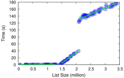
To illustrate the challenges in understanding the performance of even a sim-ple method, Figure 1.1 shows the measured running time of the C++ standard library sort method std::list<int>::sort(). We measure the running time for a range of input sizes in a controlled environment.

We run the experiments on a Intel Xeon CPU E5-2670, with 8x8GB PC4-17000 ram modules (Samsung M393A1G40DB0), whose root partition is mounted on a Samsung SSD 850 PRO drive. The OS is Ubuntu 18.04.5 LTS, and we compile the program with g++ v7.5.0-3ubuntu1 18.04, using the flags -g -O2. The system uses the default Ubuntu configuration, with the default scheduler and theintel_pstate scaling governor. We execute thesort method in a program

that we wrote for the purpose. The program first adds its pid to a

/sys/fs/c-group/memory directory to add itself to a specific Linux Control Group, then creates a list of integers with the size that is read as a command line argument. The program creates the list dynamically pushing random integers to the back of the list, and finally callsstd::list<int>::sort().

To show the interactions with the memory subsystem we limit to 52MB the amount of resident memory available to the program runningsort(using Linux

Control Groups). Using much larger inputs would have the same effect, depend-ing on the available system memory.

Despite the documented O(n log n) computational complexity of the func-tion, Figure 1.1 shows that running time has three distinct modalities: n log n for small inputs, a linear increase with a steep slope for medium-size inputs, and a dramatic jump but lower slope for large inputs. Also, not only we can observe the algorithmic complexity, but we can also see the actual absolute values that determine precisely the running time.

As long as the system has enough memory to store the entire list,sortexhibits

the expected O(n log n) time complexity. As soon as the list becomes too big (around 1.5M elements), some memory pages containing nodes of the list are swapped out of the main memory to the slower storage memory. When that happens, the time taken by Linux to store and fetch memory pages from the storage memory dominates the execution time of the algorithm, and the time complexity becomes linear. When the list becomes bigger than roughly 2.1M elements, the performance behavior in our environment changes again. Thanks to our analysis and tool, as we will show in Section 1.3, we can conclude that the big jump in the running time is still the result of the Linux memory management swapping memory pages out of the main memory. In fact, we see that the running time of the sort function exhibits a trend that is very similar to the trend seen for the number of major page faults incurred by the program.

(23)

5 1.1 Performance Analysis 0 20 40 60 80 100 120 140 160 180 0 0.5 1 1.5 2 2.5 3 3.5 T ime (s)

List Size (million)

Figure 1.1. Running time for std::list<int>::sort

with different amounts of memory (or using different sizes for the Linux Con-trol Group) would change the results considerably. The change from the first to the second modality in the performance would happen at different point on the x axis, shifting to the right with more memory and shifting to the left with less memory. Also, we can argue that running the same program with the same amount of memory on a different machine would also change the performance profile. For example using a CPU with a lower clock speed would probably in-crease the slope of the n log n part, while it would probably have little to no effect on the other parts of the graph, where the running time is mainly limited by the storage access time.

How would a programmer wanting to use this code know about these modal-ities and behaviors? The programmer could carefully study the code before using it. But apart from the fact that this would be very onerous and would lose much of the benefit of modularity, even this is not enough: the big jump in the running time is not obvious or even visible from the code, and instead is a consequence of the interaction of the code with the underlying kernel and memory subsystem. The contribution of every additional element in the list to the total running time depends on the hardware that executes the code; a different CPU executing the code might result in different slopes; a different standard library implementation might result in completely different algorithmic complexities.

In this thesis we present methodologies and tools to generate performance analyses as presented here in this example. We produce descriptions of perfor-mance with real metrics, real values for the features, and the real behavior that we extrapolate from the observations on a real system. They can include any

(24)

6 1.2 Probabilistic Performance Annotations

relevant feature, such as the length of a list, the value of an integer paramenter, or the clock speed of the CPU. And we apply this approach to every type of per-formance metric, whether it is affected by the dynamics of the system, or not.

1.2 Probabilistic Performance Annotations

With our performance analysis we combine and improve every aspect of the pro-filers and empirical models developed in the past, as described in Chapter 2.

At a high level, our approach works as follows. We collect performance data (e.g., CPU time, memory usage, lock holding/waiting time, etc.) along with features of the arguments to functions (e.g. value of an int, length of a string, etc.) or of the system (e.g. CPU clock speed, network bandwidth, etc.). We then use statistical analysis to build mathematical models relating input features to performance. We produce performance annotations at the method granularity. In other words, our performance annotations always refer to named software routines, which take a set of input parameters, and produce some output before finishing their execution.

We produce cost functions for different performance metrics. These cost func-tions correlate concrete performance metrics to features of different nature. As we already discussed, cost functions are more informative than the aggregate metric data produced by traditional profilers.

Similarly to traditional profilers, we analyze real performance metrics, and whether they are affected by the dynamical aspects of the system, or not. This choice is at the base of two important features of our performance annotations: (1) performance annotations are probabilistic, to handle and represent the noise that stems from the dynamical aspects of a system, and (2) performance anno-tations use scopes to represent the multi-modal performance behaviors, whether they are due to the algorithm or to the interaction of the target program with the rest of the system.

Let’s see a real example of performance annotation, for the example of the

std::list<int>::sort method shown in Section 1.1. Remember that we are artificially limiting the amount of memory to make the sort method swap memory to the main storage, and this induces different modalities in the running time of the method for different list sizes.

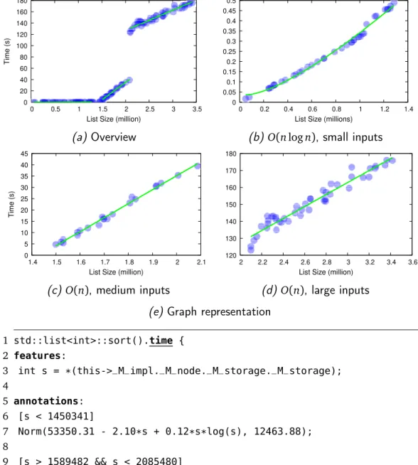
Figure 1.2 shows the concrete output of our analysis for the running time. It consists of a textual representation (Fig. 1.2f), and a graphical one (Fig. 1.2e).

The performance annotation shows that the running time metric is mainly affected by the size of the list. The cost functions show that the performance

(25)

7 1.2 Probabilistic Performance Annotations 0 20 40 60 80 100 120 140 160 180 0 0.5 1 1.5 2 2.5 3 3.5 T ime (s)

List Size (million)

(a) Overview 0 0.05 0.1 0.15 0.2 0.25 0.3 0.35 0.4 0.45 0.5 0 0.2 0.4 0.6 0.8 1 1.2 1.4

List Size (millions)

(b)O(n log n), small inputs

0 5 10 15 20 25 30 35 40 45 1.4 1.5 1.6 1.7 1.8 1.9 2 2.1 T ime (s)

List Size (million)

(c)O(n), medium inputs

120 130 140 150 160 170 180 2 2.2 2.4 2.6 2.8 3 3.2 3.4 3.6

List Size (million)

(d) O(n), large inputs (e) Graph representation

1 std::list<int>::sort().time { 2 features: 3 _{int s = *(this->_M_impl._M_node._M_storage._M_storage);} 4 5 annotations: 6 [s < 1450341] 7 _{Norm(53350.31 - 2.10*s + 0.12*s*log(s), 12463.88);} 8 9 [s > 1589482 && s < 2085480] 10 _{Norm(-90901042.29 + 63.11*s, 899547.29);} 11 12 [s > 2098759] 13 _{Norm(56712024.50 + 35.38*s, 3379580.27);} 14 } (f) Textual representation

(26)

8 1.2 Probabilistic Performance Annotations

complexity is O(n log n) for lists of less than 1450341 elements, while it becomes O(n) for bigger inputs. Since the correlation is not perfect and there is some noise around the expected performance cost, our cost functions contain random variables. In this case the random variable has a normal distribution with a known mean that depends on the size feature, and a known variance.

We believe that any developer or analyst with some domain knowledge would be able to read and interpret the performance annotation easily, without any in-depth knowledge of our annotations language.

Notice how the main feature, the list size, is expressed with the exact name that the feature has in the program that is being analyzed. Thus the meaning of the feature should be immediately clear to the developer.

The graph contains the visual representation of the performance annotation, that is, the set of cost functions, and the set of observations that were used to infer such function. To the human analyst, the graph is even more immediate to interpret than the formal performance annotation,

The graphical representation is very useful to human users and are a very effective documentation of the performance behavior, while the textual repre-sentation can be efficiently parsed by computers, and make the ideal base for assertion checking.

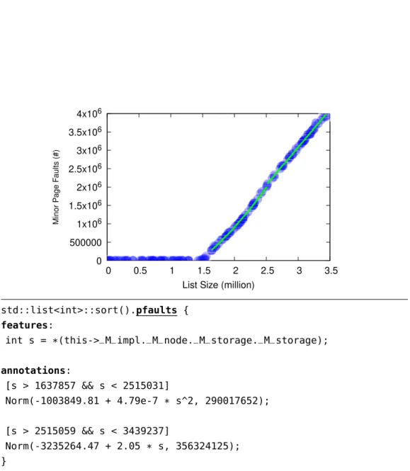
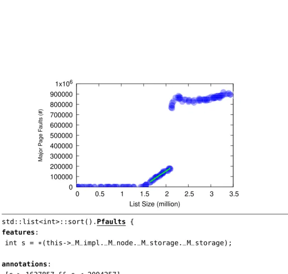
In order to have a better understanding of the nature of the different modal-ities in the running time, we produce the performance annotations forsortalso

for two additional performance metrics: minor page faults (Figure 1.3), and ma-jor page faults (Figure 1.4).

These performance annotations confirm that indeed there are zero major page faults when the list fits entirely in memory. Also, when the memory is not enough to store the entire list, the number of minor page faults grows almost linearly with the size of the list. It is very interesting to see that the growth is slightly more than linear when the list has around 220_elements.

At the same time it is clear that it is the number of major page faults that affects the running time of the sortfunction the most. Guided from the

perfor-mance annotations, we run more experiments manually to see that the big jump in the major page faults (and in the running time) happens exactly when the list contains 221_{+1 elements. Observing Figure 1.2b more carefully, we can notice a}

smaller jump in the running time when the list contains exactly 220_{+1 elements.}

These observations lead us to think that the big jump in the number of memory page faults is not only related to the amount of resident memory available to the program, but also to other factors, like the size of the cache memory of the CPU, or the effect of the algorithm on the memory pages.

(27)

9 1.2 Probabilistic Performance Annotations 0 500000 1x106 1.5x106 2x106 2.5x106 3x106 3.5x106 4x106 0 0.5 1 1.5 2 2.5 3 3.5 Mi n or P a g e F a ul ts (# )

List Size (million)

1 std::list<int>::sort().pfaults { 2 features: 3 _{int s = *(this->_M_impl._M_node._M_storage._M_storage);} 4 5 annotations: 6 [s > 1637857 && s < 2515031] 7 _{Norm(-1003849.81 + 4.79e-7 * s^2, 290017652);} 8 9 [s > 2515059 && s < 3439237] 10 _{Norm(-3235264.47 + 2.05 * s, 356324125);} 11 }

(28)

10 1.2 Probabilistic Performance Annotations 0 100000 200000 300000 400000 500000 600000 700000 800000 900000 1x106 0 0.5 1 1.5 2 2.5 3 3.5 Ma jo r P a g e F au lt s (#)

List Size (million)

1 std::list<int>::sort().Pfaults { 2 features: 3 _{int s = *(this->_M_impl._M_node._M_storage._M_storage);} 4 5 annotations: 6 [s > 1637857 && s < 2094257] 7 _{Norm(-431212.95 + 0.23 * s, 19540310);} 8 }

(29)

11 1.3 Freud

human performance analyst, our analysis can be applied to much more com-plex cases with similar results, as we will show in the experimental evaluation presented later in Chapter 6.

Again, one of the key advantages of our analysis is that it can be performed automatically, minimizing the input requested to the user. This avoids human error, makes the adoption of the performance analysis more likely, and opens new possibilities in terms of automation and integration of performance analysis in common development practices. Indeed, the graphs and textual annotations showed in Figures 1.2-1.4 were generated automatically by our tool, Freud.

1.3 Freud

Freud performs the analysis automatically. The user is not required to have any knowledge of the program under analysis, to create semantically meaningful per-formance annotations. The only input taken by Freud are (1) the binary of the target program compiled with debugging symbols, (2) the names of the meth-ods (or “symbols”) that shall be analyzed, and (3) the performance metrics of interest. Also, if necessary, the workload that is processed by the target program has to be provided. We do not provide any recipe for the creation of workloads triggering interesting performance behavior.

As we will detail in Chapter 5, Freud uses different approaches to infer the different modalities in the performance behavior automatically, regardless of the origin of the multi-modal behavior.

Concretely, Freud consists of a set of tools. On the one side there are instru-mentation modules, that find and extract data from a running program. On the other side there is the analysis module, which performs a statistical analysis on the data collected by the instrumentation.

The statistical analysis is generic. As longs as the data collected by the instru-mentation is provided in the correct format, the analysis can work with software written in any language.

The instrumentation part is necessarily language specific. We have imple-mented a prototype for C/C++ code, that uses Intel Pin [35] to dynamically in-strument the target program. The choice of the C/C++ programming language is motivated by several factors.

C++ is the language used for most of the performance critical software. It is extensively used by the industry in many different areas. Also, C is probably one of the most difficult programming language to analyze for our purpose of creating performance specifications. In particular, C has a type system that

(30)

en-12 1.4 Contribution and Structure of the Thesis

forces only a weak form of type safety that can in any case be circumvented. In other words, we give a reference implementation for a difficult language, and therefore argue that creating instrumentation tools for other, stricter languages should be relatively easy.

Concretely, to create a performance annotation for the std::list::sort

function, the performance analyst would:

1. compile the program that uses thesort function with debugging symbols (usually passing the -g flag to the compiler)

2. run the Freud binary analyzer (freud-dwarf) on the binary file that contains the compiled program

3. compile the PinTool using the instrumentation code generated in step 2 4. run the instrumented program multiple times with Intel Pin (freud-pin),

executing the sort function with diverse inputs

5. run the Freud statistical analyzer (freud-statistics) on the logs collected in step 4

We developed Freud with the ideal goal of making it reasonable efficient to be used in a production environment. In this way Freud could continuously collect new data, to react to unexpected performance behaviors as soon as they hap-pen. For this purpose, we tried different approaches to minimize the overhead introduced by Freud.

1.4 Contribution and Structure of the Thesis

In essence, this thesis describes systems work. We develop a new model for per-formance analysis with a very practical approach. Indeed the requirements and the development of the model have been driven by real-world cases of complex performance analysis. We also present a real, open-source prototype that per-forms performance analysis of complex software using most of the features of our performance modeling language.

In summary, this thesis makes the following contributions:

• We compare our approach and tool for performance analysis to the models and tools developed in the past (Chapter 2);

• We develop a performance model in the form of probabilistic performance annotations. In Chapter 3 we detail the features and the language used for our model formally;

(31)

13 1.4 Contribution and Structure of the Thesis

• We describe a methodology to derive performance annotations through dy-namic analysis. In particular, our techniques can automatically identify rele-vant features of the input, and relate those features through a synthetic statis-tical model to a performance metric of interest (Chapter 4);

• We describe a concrete implementation of the methodology in a tool named Freud, which automatically produces performance annotations for C/C++ programs (Chapter 5);

• We evaluate Freud through controlled experiments, and analyze two complex systems: MySQL (written in C++), and the x264 video encoder (written in C). We also show how the same analysis can be applied with promising results also to the ownCloud storage service, which is a web application written in PHP (Chapter 6).

(32)

(33)

Chapter 2 Related Work

A lot of research spanning several decades has focused on performance analysis for software systems. Indeed, optimizing algorithms and their implementations to reduce resource usage is one of the driving factors in software development and computer science generally, both for performance-critical applications and not. Hardware and software profilers already existed in the early 70s, allowing the programmer to identify hot spots and bottlenecks in their programs. For example, the Unix prof command already appears in the 4th edition of the Unix Programmer’s Guide, dated 1973.

Given the number of publications and authors working on performance anal-ysis in the past, there are different possible ways of classifying the previous ap-proaches. Examples are the surveys by Balsamo et al. [2] and Koziolek [26].

The first distinction that we can make between different approaches to per-formance modeling, is that of static models as opposed to empirical models.

Static models (e.g. [5, 13, 47, 18, 4]) are designed to be used without any concrete implementation of the program. The main advantage is that they can be employed in the early design phases of software. These models typically rep-resent software as a network of boxes, either extending UML diagrams or using ad-hoc modeling languages. Each box represents a software component, and is characterized by a user provided performance profile. These models typically provide tools to compose the behavior of different components in the system (e.g., the runtime needed to access the database) to infer and predict the over-all performance of the complete software system (e.g., the end-to-end latency to serve a user request).

Conversely, empirical models (e.g. [30, 29, 33]) are created through obser-vation of real software. These models typically instrument or augment existing software to extract performance information while the software runs. It goes

(34)

16 2.1 Traditional Profilers

without saying that these models need a concrete implementation of the soft-ware, but have many advantages over static approaches. The amount and quality of information that can be collected is much higher, and the analysis can be auto-mated, reducing the need for any user input, which can be costly and is anyway subject to human errors.

We now focus exclusively on empirical approaches to software modeling. In-deed, this is the approach that we take with our performance annotations. In the following sections we describe part of the research efforts in the field of software performance. Besides traditional profilers (Section 2.1), software engineering research has developed several ideas and tools to assert (Section 2.2) or infer (Section 2.3) software performance. Most of these efforts resulted in some pro-totype implementations of the ideas. Finally, Section 2.4 and Section 2.5 show examples of research papers that discuss two of the immediate extensions of this work, namely distributed instrumentation and performance prediction on differ-ent hardware. In Section 2.6 we briefly compare all these implemdiffer-entations to Freud, our tool to generate performance annotations.

2.1 Traditional Profilers

Today, developers rely on profilers like gprof [17] or JProfiler [24] to understand the performance of their code.

Traditional profilers measure the execution cost (e.g., running time, executed instructions, cache misses) of a piece of code. The profiler would typically access information about function calls and periodically sample the program counter to observe which function of the program is being executed. Knowing the total running time for the program, the profiler computes aggregate statistics on func-tions, indicating for example that function f was called a total of 1000 times, that 10% of program execution time was spent in function f , and that invocations of function f took 4ms on average.

The information the gathered and summarized by the profiler might be in-sufficient in some scenarios. Consider the sort example above: not only a

tra-ditional profiler would have no information about the different modalities, but the output produced would probably be misleading. The aggregate information about the runtime would show only the total time spent in the sort method dur-ing the execution of the program, and the number of calls, indicatdur-ing an average execution time but not its variance.

Since the variance in the running time is large (it ranges from 0 to 180 sec-onds), the aggregate information would fail completely in describing the real

(35)

17 2.2 Performance Assertion Specification

performance, suggesting an expected running time much higher than what it is in reality.

Traditional profilers do not relate the performance of a method to its input and offer no predictive capabilities. Also, traditional profilers generate informa-tion that is specific not only to a particular executable program, but also to a specific run (one or more) of the program. This means that a profiler shows in-formation that is potentially affected by a specific context (e.g. the number of CPUs, the size of the input passed to the program, . . . ), without collecting any information about such context. This means that the data collected with profil-ers is useful only to the user of the profiler who ran the experiments, since the results depend on information that is usually not provided with the analysis.

DTrace and Perfplotter are more advanced tools that extend the capabilities of traditional profilers in different directions.

DTrace [8] represents one of the first attempts to instrument production sys-tems, with zero overhead on non-probed software components. DTrace intro-duces a new language, calledD, to let users write their own instrumentation code,

which can access information in the user-space or in the kernel space. With theD

language, performance analysts can either produce aggregate information about a finite set of executions of a given method, or produce specific information about every single execution. On the other hand, both the selection of the information to collect and the analysis of the raw data are a responsibility of the users of DTrace. While DTrace was originally written for Solaris, several ports exist for different operating systems, including Linux. On the other hand, DTrace relies on its own kernel module to work, which is not in the Linux mainline repository, possibly limiting the adoption of the tool.

Perfplotter [9] uses probabilistic symbolic execution to compute performance distributions for Java programs. Perfplotter, which takes as input Java Bytecode, a usage profile, and outputs performance distributions. Perfplotter uses symbolic execution, in conjunction with the usage profile, to explore all the most common execution paths in the Java byte-code. Every unique path is executed a number of times with varying input parameters, and the average execution time is mea-sured and associated with that path. The output distribution shows the average execution time and the probability of being executed for each path.

2.2 Performance Assertion Specification

PSpec [34] introduces the idea of assertions that specify performance properties. PSpec is a language for specifying performance expectations as automatically

(36)

18 2.2 Performance Assertion Specification

checkable assertions.

PSpec uses a trace of events produced by an application or system (e.g., a server log). Developers modify their programs to produce event traces in the cor-rect form. These traces amount to a sequential list of typed events. Each event type has a unique name and a user-defined set of attributes. Basic attributes in-clude the thread_id, the processor_id, and the timestamp. Other attributes might include the size of an input, the name of a file, and so on.

Developers manually specify performance assertions in the PSpec language. They first define an interval, identified by a pair (start_evt, end_evt). For each interval they can specify a metric computed as a function of some attributes of some events. For example, a simple metric would be running time, computed as timestamp(end_evt) − timestamp(start_evt). For each interval, users of PSpec can write assertions using the attributes of the events defining the interval. The assertions can include unknown variables that can be assigned by the checker tool provided by PSpec. PSpec also provides the where keyword, which can be used in assertions to filter the intervals for which the assertion is checked.

Finally, PSpec provides the checker tool, that processes logs and the perfor-mance specifications to validate the assertions.

Vetter and Worley [45] use assertions that are added to the source code of the target program by the performance analyst. Assertions apply to specific code segments identified by the keywordspa_startandpa_end, and can access a

pre-defined list of hardware performance counters, in addition to any user-pre-defined feature that is passed to the performance assertion explicitly in the code. Vetter and Worley develop a runtime system that applies the optimal instrumentation to extract the metrics requested by the user in the most efficient way. Assertions are evaluated at runtime while the target program is executing.

Since performance assertions integrate natively with the source code of the target program, developers can use the result of the assertions directly in their programs, reacting to the outcome of the assertions. This approach requires a tight integration with the specific programming language of the target program. The authors implemented the runtime as a library for C, but argue that integrat-ing their code in the compiler might be a viable alternative.

Both of the above approaches allow developers to specify fixed bounds for the values of chosen metrics in their assertions (e.g., on running time), but do not provide a statistical approach based on the distribution of those metrics. Also, the approaches require a manual specification of the performance models/assertions. Finally, the approaches described in this section require the availability of the source code of the target program, so that the program can be augmented and recompiled with the required instrumentation specifications.

(37)

19 2.3 Deriving Models of Code Performance

2.3 Deriving Models of Code Performance

Trend Profiling [16], Algorithmic Profiling [49] and Input-Sensitive Profiling [11, 12] represent a new form of profiling: instead of only measuring the execution cost, these profilers characterize a specific cost function, namely a relationship between input size and execution cost. They produce profiles such as: function

f takes 5 + 3i + 2i2 _{ms, where i is the length of the input array.}

Besides the common goal of inferring performance cost models, these ap-proaches have a number of differences:

• Granularity: Trend Profiling and Algorithmic Profiling analyze sub-routine code blocks, while Input-Sensitive profiling considers complete routines. • Feature discovery: Trend Profiling does not make any attempt at finding

relevant features, and relies completely on the input provided by the user. Algorithmic Profiling and Input-Sensitive profiling, instead, try to find the relevant feature automatically.

• Feature types: While the definition of a feature is left to the user of Trend Profiling, both Algorithmic and Input-Sensitive profiling use a notion of size as the only feature affecting performance. Algorithmic Profiling com-putes the size of the data structures that are used either as input or output by the code block under analysis, while Input-Sensitive profiling considers the number of memory cells accessed. None of these profilers account for multiple feature when computing cost models.

All these algorithmic profilers consider the number of executions of basic blocks or loop iterations as the performance metric. While this performance metric has the advantage of not being subject to noise in the measurement, and thus being good for analyzing the asymptotic performance behavior of software, it also has serious limitations.

Again, this kind of analysis would be limiting in our sort example. We would only see the O(n log n) algorithmic complexity, but we would have no signs of the different modalities, since the interaction with the memory subsystem would be completely ignored. Moreover, we would have no idea of the actual time spent executing the function. Our work complements algorithmic profilers in that, rather than using an abstract notion of complexity, it considers real performance metrics and also the interaction of the code with the underlying hardware and software.

(38)

20 2.4 Distributed Profiling

2.4 Distributed Profiling

While we do not consider the problem of distributed instrumentation directly in this dissertation, extending our analysis to distributed systems is clearly a pos-sible future extension. In fact, using distributed instrumentation to be able to collect more potential features would greatly extend the possible uses and appli-cability of our analysis.

Distributed profiling allows instrumenting distributed systems to correlate events happening on physically or logically different nodes of the distributed system. Recent architectures running cloud services often run in big data centers, where interactive software components run on virtually and physically different machines. Still, it is usually essential for the developers and performance analysts to be able to correlate events observed on one server to events observed on a different server.

The first documented system in order of time that has this precise goal is Magpie ([3]). The authors wanted to measure the end-to-end performance of a web service from the user’s perspective. To do that, Magpie tags incoming requests with a unique id, and then propagates this id throughout the processing steps required to fulfill the request.

Dapper [38] takes a very similar approach. Dapper is a low-overhead in-strumentation system developed and used internally by Google within their pro-duction data centers. Dapper provides precious functional and performance de-bugging information to developers by continuously and transparently recording traces for requests entering a data center. In particular, Dapper instruments a small set of flow-control Python libraries that run at a low level of the software stack and that are used by most of the higher level software components across the Google data centers. Similar to Magpie, the instrumented version of the li-braries appends a trace id to every RPC call that is then shared and propagated for all the follow up requests related to the original transaction. In order to limit the overhead brought by the instrumentation, Dapper allows sampling of the traces. Interestingly, researchers at Google claim that analyzing one out of a thousand requests is sufficient to characterize precisely the workflow on their systems.

More distributed instrumentation tools that implement the same ideas are Twitter’s Zipkin [43], Uber’s Jaeger, and OpenTracing.

Mace at al. combine dynamic instrumentation techniques with distributed instrumentation in their tool Pivot Tracing [28]. This tool uses the established distributed profiling technique of associating requests entering the system with uniquely identifying metadata tags, which are propagated along with the request in the distributed system. Performance analysts, who must have a good

(39)

knowl-21 2.5 Hardware Aware Performance Specifications

edge of the system, define tracepoints. A tracepoint is a specification containing information on where, in the distributed system, to add jumps to the instru-mentation code. Such instruinstru-mentation code is created by Pivot Tracing from the user-defined specification of which input parameters to collect from software method being instrumented. Pivot Tracing enables dynamic instrumentation of a distributed systems, allowing performance analysts to collect requested infor-mation, optionally including causal relationships between different events, from the system.

2.5 Hardware Aware Performance Specifications

Finally, while we do not experiment directly with hardware with different archi-tectures in this thesis, we think that it is possible to consider hardware specifi-cations as additional features that Freud can analyze to document and predict performance. Some recent research papers explored similar ideas, and proved effective.

Valov et al. [44] show that it is possible to build linear transfer models that allow to predict with good accuracy the performance metrics from one specific hardware configuration to a different one. The approach is still limited in many ways. It considers only the running time as a performance metric. Moreover, the transfer models it produces are effective only over similar hardware, for which linear transformations are appropriate. This is limiting because, in reality, spe-cific hardware architectures could be used to speed up the execution of spespe-cific tasks with super-linear improvements. One example is the use of GPUs to encode a video stream to h264.

Thereska et al. [41] introduce the notion of performance signatures. A perfor-mance signature is a collection of key-value pairs that describe a specific system in a specific state. For example, a performance signature may state that an in-stance of Microsoft Excel is saving a 100KB file to the filesystem, on a 2-cores x86 machine, with 2GB of RAM. These performance signatures can be generated and collected by Microsoft software that have specific debugging flags activated by the user. Once the authors have collected metrics from thousand of deploy-ment around the world, they make predictions picking the signature that is the closest to the signature of the hypothesis. The distance between two signatures is computed as a summation of the distances of specific (static) features of the signatures, where each feature is assigned a weight chosen by the analyst.

(40)

22 2.6 Comparison with Freud

2.6 Comparison with Freud

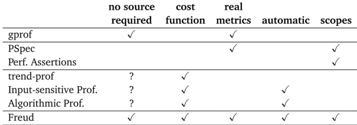
Table 2.1 summarizes the main differences between Freud and the previous ap-proaches to performance analysis.

no source cost real

required function metrics automatic scopes

gprof Ø Ø PSpec Ø Ø Perf. Assertions Ø trend-prof ? Ø Input-sensitive Prof. ? Ø Ø Algorithmic Prof. ? Ø Ø Freud Ø Ø Ø Ø Ø

Table 2.1. Comparison of different approaches to performance analysis

It is clear from the table that we are trying to combine all the good features of the previous performance models into one method and tool. The reason that this has not been done before is that these features introduce competing challenges. For example, computing cost functions conflicts with using real metrics, for the reasons that we discussed already (noise and modalities). Similarly, the automa-tion of the analysis conflicts with the descripautoma-tion of scopes in the performance behavior, since multi-modal behaviors make the analysis much more difficult.

To recap, Freud expands on the previous ideas in four ways: (1) Unlike al-gorithmic profiling, which measures cost in terms of platform-independent iter-ation counts, we measure real performance metrics. (2) The domain of the cost function in algorithmic profiling is the size of a data structure. In input-sensitive profiling, it is the number of distinct accessed memory locations. In contrast, our performance annotations can include arbitrary features of the executing pro-gram, or of the system on which it is running. (3) Algorithmic and input-sensitive profiling produce cost functions, but the specific approach for fitting a cost func-tion to the measurements is outside the scope of that work. Freud automati-cally infers cost functions from the measured data points, producing complete formal performance annotations. (4) Code often exhibits different performance modes (e.g., slow and fast paths), and Freud is able to automatically partition the measurements and to model them as sets of scoped cost functions; prior work produces a single cost function.

Also, many performance models use static features, such as calling context [7], application configuration [19], OS version [42], or hardware platform [22].

(41)

23 2.6 Comparison with Freud

In contrast, Freud uses the dynamic state of the running system, i.e., the fea-tures that most directly affect computational complexity and are most relevant for scalability.

Finally, despite the semantic richness of the performance annotations created, Freud does not need the source code for C/C++ programs to perform its analysis. All the information needed are extracted from the debugging symbols integrated with the binary of the target program.

(42)

(43)

Chapter 3 Performance Annotations

In this chapter we describe the notion, the language, and the uses of proba-bilistic performance annotations. In Section 3.1 we present the syntax of the performance annotation language, and we show through a series of examples what can be expressed with performance annotations. Section 3.2 then shows how performance annotations can be used in different scenarios and for different purposes, such as documentation and performance assertion checking.

While in this thesis we introduce both a language for performance specifi-cations and a tool to automatically generate such specifispecifi-cations, in this chapter we describe the language with all the features we developed for it to describe the performance behavior of any software. Some of these features, such as the composition of different performance annotations, are not yet used (i.e., not im-plemented) by our tool.

3.1 Performance Annotations Language

We design a language for performance annotations intended for both human engineers and automatic parsing and processing. The language defines concrete metrics, such as run-time or allocated memory, to characterize the performance of a module or function. An annotation expresses one or more relations between one such metric and features of the input or state of the module or function. A typical input feature is a parameter of the module or function being annotated.

The performance annotation language must include parts of the language of the program under analysis. The metrics and the expressions that characterize them are independent of the program, but the identification of the function or module, as well as their input or state features are expressed in the language of the program.

(44)

26 3.1 Performance Annotations Language

3.1.1 Structure

Performance annotations are composed of three distinct parts: (1) signature, (2) features, and (3) annotations.

The signature introduces the annotation and uniquely identifies a method or function as it appears in the instrumented program, typically with the method name and the list of formal parameters. The signature also indicates which per-formance metric the annotation describes.

The second part lists all the features that are used in the performance annota-tion. Each feature is defined by a type, a name, and an initialization expression:

type name=definition-expression;

The type can bebool,int,float, orstring; name is an identifier used to refer

to that feature in the performance annotation; and definition-expression defines the feature in terms of the program under analysis, typically in terms of input pa-rameters and other variables accessible within the annotated method or function. Therefore, the definition expression is written is the programming language of the target program, and should be easy to read and interpret by the performance analyst and the developer of the program.

The third and last block describes the behavior of the annotated method or function with a list of expressions. This is the central part of a performance annotation. Each expression characterizes the indicated performance metric as a random variable (the dependent variable) whose distribution is a function of zero or more of the listed features (the independent variables). Thus, in essence, a performance annotation is an expressions like the following:

Y ∼ expr(X)

which is read as: Y is a random variable distributed like expr(X ), where X is the set of relevant features. Expressions with zero input features describe behaviors that are independent of the input or for which no relevant features have been observed.

The characterization of each performance metric amounts to the total cost of an execution of the annotated method or function, including all the costs incurred by other methods or functions that are directly or indirectly within the annotated method. Using the terminology of the gprof profiler, we describe the total cost of the method, as opposed to the self cost.

We now present concrete examples of performance annotations to illustrate all the features the language. We will use performance annotations that we cre-ated for real software chosen from well known software libraries or programs.

(45)

3.1.2 Basics

Figure 3.1 shows a first basic example of a performance annotation for thesort()

method of thelist<int>_{class of the C++ Standard Library (libstdc++ v6.0.24).}

The annotation describes the running time of std::list<int>::sort() with

workloads that impose no memory constraints and that require no memory swap-ping. 1 std::list<int>::sort().time { 2 features: 3 _{int s = *(this->_M_impl._M_node._M_storage._M_storage);} 4 5 annotations: 6 _{Norm(0.15*s*log(s), 72124.40)} 7 }

Figure 3.1. A performance annotation with regressions

Line 1 introduces the annotation with the signature of the target method and the performance metric under analysis denoted by the time keyword. The unit of measure for a performance metric is implicitly defined by the metric. In this case for running time the unit is 1µs (microseconds). Table 3.1 shows the metrics that we consider in the current version of the annotation language together with the corresponding keywords and units of measure.

Line 3 defines a feature s of type int used in this performance annotation. The definition of the feature_{*(this->_M_impl._M_node._M_storage._M_storage)} is written in the language of the target program and uses the exact names of variables and struct members that refer to the relevant feature as they would be interpreted in the program and in particular in the scope of thesortmethod.

metric keyword units

running time time microseconds

lock waiting wait microseconds

lock holding hold microseconds

memory mem bytes

minor page faults pfaults number

major page faults Pfaults number

(46)

Specifically, since we are analyzing a C++ program and sincesortis a non-static

method of thestd::listclass,thisrepresents a pointer to thestd::list

ob-ject on which sort is called. In particular, the definition of the feature is an r-value expression that identifies an int object that can be read within the instru-mented target program at the time of the execution of the annotated method.

In essence, the annotation states that the running time oflist<int>::sort

depends on a state variable of the list object on which it is called, and as it turns out that state variable represents the number of elements in the list.

Finally, the expression on line 6 of Figure 3.1 characterizes the indicated per-formance metric with the given feature. This is an example of the general expres-sion Y ∼ expr(X ) introduced above. In this case, the annotation states that the running time is a random variable with a normal distribution whose mean grows as s log s and whose variance is known, where s is the size of the list. Notice that the annotation expression does not only define the asymptotic, big-O complexity of the method, but it also defines an actual coefficient for the expected growth rate, which corresponds to the concrete values of the performance metric (time) in its predefined unit of measure (microseconds).

Notice that in this example and in the rest of this document we represent floating-point numbers with a few decimal digits. This is solely for presentation purposes, and is not a limit of the language or its implementation.

3.1.3 Modalities and Scopes

Oftentimes software functions exhibit different modalities in their performance behavior. There are two different sources for such variability: (1) the algorithm takes different paths in the execution depending on the input it reads, or (2) the interaction of the algorithm with the rest of the system on which it is running. More about the sources of multi-modal behaviors will be in Chapter. 4. In this section we will discuss the features of the language that allow to account for and describe this variability, regardless of its nature.

Performance annotations account for multi-modal performance behaviors by means of scope conditions. With scope conditions we want to express cases in which the occurrence of a specific distribution for the performance behavior is tied to the validity of a specific condition (the scope). For example, we have:

Y ∼ [C1] expr1(X1); [C2] expr2(X2); . . . ; [Cn] exprn(Xn);

This means that the performance metric Y follows the distribution expr₁(X1)

(47)

Going back to thestd::list<int>::sort function, we limit the amount of

resident memory that the program can use. Again, we deliberately set a limit (of 36MB) to cause memory swapping. We make the sort function behave as we showed in Figure 1.1, in Chapter 1. The performance annotation becomes the following: 1 std::list<int>::sort().time { 2 features: 3 _{int s = *(this->_M_impl._M_node._M_storage._M_storage);} 4 5 annotations: 6 [s < 1450341] 7 _{Norm(53350.31 - 2.10*s + 0.12*s*log(s), 12463.88);} 8 9 [s > 1589482 && s < 2085480] 10 _{Norm(-90901042.29 + 63.11*s, 899547.29);} 11 12 [s > 2098759] 13 _{Norm(56712024.50 + 35.38*s, 3379580.27);} 14 }

Figure 3.2. A performance annotation with regressions

We see that the relevant feature for the running time is still the length of the list. This time, though, we observe three different modalities in the behavior of the method. Each modality is described by a different expression, and a scope. Each scope describes the condition that must evaluate to true for the expressions in the following lines to be representative of the expected behavior. As example, line 6 states that if the length of the list (s) is smaller than 1450341, then the

expected running time for the sort method is the one expressed at line 7. This is exactly what we expect: if the list fits entirely in memory, the running time for

sort grows as n log n with the length of the list.

Similarly, at line 9 we have the condition in which the second modality is observed (linear increase, high slope, line 10). Finally at line 12 we have the condition in which the third modality is observed (linear increase, lower slope, line 13).

In all three cases, the performance annotation uses a normal distribution. In the first case, ignoring the constants, we see that the mean value is n log n where n is the length of the list being sorted, which conforms to the expected O(n log n)

(48)

complexity. In the second and third cases, the performance is linear with the length of the input list but with different constant values.

When a specific feature is not present in a scope condition, its value is ir-relevant for the evaluation of the condition. The union of all the scopes in one performance annotation covers the entire input domain of the function, while their intersection is empty. In other words, scopes represent a partitioning of the input domain of the function that is described by the performance annota-tion. As we will see in the following Chapter, the annotation describes a type of classification tree where the scope conditions indicate partitions.

While in Figure 3.2 the scope conditions contain only one variable/feature, there is no such limit in general. For example, one scope condition of a perfor-mance annotation could state[ s < free_mem ].

3.1.4 Mixture Models

Expressions with zero input features describe behaviors that are independent of the input or for which no relevant features have been observed.

In the previous examples we always had performance annotations using at least one feature, used in the performance expressions to characterize the ex-pected performance behavior.

In other cases we might have performance annotations that do not use any feature. While such annotations carry less information about the trends in the performance behavior of functions, they might still describe different modalities. In such cases, performance annotations resort to probabilities of occurrence to describe the different modalities. More formally, performance annotations allow expressions like the following:

Y ∼ {p1}expr1; {p2}expr2; . . . ; {pn}exprn;

where each pi represents the probability that the performance metric is

dis-tributed like expr_i. When a performance annotation specifies probabilities, it must cover the entire space of behaviors. In other words, Pn_i=1p_i = 1.

Here is a concrete example of a performance annotation that does not use any features, but still describes a multi-modal behavior through probabilities: