Systematics of central heavy ion collisions in the 1A GeV regime

arXiv:1005.3418v2 [nucl-ex] 13 Sep 2010

Systematics of central heavy ion collisions in

the 1A GeV regime

W. Reisdorf,

, A. Andronic

, R. Averbeck

,

M.L. Benabderrahmane

, O.N. Hartmann

, N. Herrmann

,

K.D. Hildenbrand

_{, T.I. Kang}

_{, Y.J. Kim}

_{, M. Kiˇs}

_,

P. Koczo´

n

, T. Kress

, Y. Leifels

, M. Merschmeyer

,

K. Piasecki

, A. Sch¨

uttauf

, M. Stockmeier

, V. Barret

,

Z. Basrak

, N. Bastid

, R. ˇ

Caplar

, P. Crochet

,

P. Dupieux

, M. Dˇzelalija

, Z. Fodor

, P. Gasik

,

Y. Grishkin

, B. Hong

, J. Kecskemeti

, M. Kirejczyk

,

M. Korolija

, R. Kotte

, A. Lebedev

, X. Lopez

,

T. Matulewicz

, W. Neubert

, M. Petrovici

, F. Rami

,

M.S. Ryu

, Z. Seres

, B. Sikora

, K.S. Sim

, V. Simion

,

K. Siwek-Wilczy´

nska

, V. Smolyankin

, G. Stoicea

,

Z. Tymi´

nski

, K. Wi´sniewski

, D. Wohlfarth

, Z.G. Xiao

,

H.S. Xu

_{, I. Yushmanov}

_{, A. Zhilin}

(FOPI Collaboration)

a_{GSI Helmholtzzentrum f¨ur Schwerionenforschung GmbH, Darmstadt, Germany} b_{National Institute for Nuclear Physics and Engineering, Bucharest,Romania}

c_{Central Research Institute for Physics, Budapest, Hungary}

d_{Clermont Universit´e, Universit´e Blaise Pascal, CNRS/IN2P3, Laboratoire de}

Physique Corpusculaire, Clermont-Ferrand, France

e _{Institut f¨ur Strahlenphysik, Forschungszentrum Rossendorf, Dresden, Germany} f_{Physikalisches Institut der Universit¨at Heidelberg,Heidelberg, Germany}

g_{Institute for Theoretical and Experimental Physics, Moscow,Russia} h_{Kurchatov Institute, Moscow, Russia}

i_{Institute of Modern Physics, Chinese Academy of Sciences, Lanzhou, China} j_{Korea University, Seoul, South Korea}

k_{Institut Pluridisciplinaire Hubert Curien, IN2P3-CNRS, Universit´e de}

Strasbourg, Strasbourg, France

ℓ_{Institute of Experimental Physics, University of Warsaw, Poland} m_{Rudjer Boskovic Institute, Zagreb, Croatia}

Abstract

Using the large acceptance apparatus FOPI, we study central collisions in the re-actions (energies in A GeV are given in parentheses): 40_Ca+40_{Ca (0.4, 0.6, 0.8,} 1.0, 1.5, 1.93), 58_Ni+58_{Ni (0.15, 0.25, 0.4),} 96_Ru+96_{Ru (0.4, 1.0, 1.5),} 96_Zr+96_Zr (0.4, 1.0, 1.5),129Xe+CsI (0.15, 0.25, 0.4),197Au+197Au (0.09, 0.12, 0.15, 0.25, 0.4, 0.6, 0.8, 1.0, 1.2, 1.5). The observables include cluster multiplicities, longitudinal and transverse rapidity distributions and stopping, and radial flow. The data are compared to earlier data where possible and to transport model simulations.

Key words: heavy ions, rapidity, stopping, viscosity, radial flow, cluster production, nucleosynthesis, nuclear equation of state, isospin

PACS: 25.75.-q, 25.75.Dw, 25.75.Ld

1 Introduction

In the past twenty five years studies of nucleus-nucleus collisions over a very broad range of energies have been performed. The goal was, and still is, to learn more about the prop-erties of hot and dense nuclear matter, namely its equation of state (EOS) and transport coefficients such as viscosity and thermal conductivity. In the energy range (0.1 to 2A GeV) of the Schwerionen Synchrotron (SIS) accelerator located at GSI, Darmstadt, one expects from simple-minded hydrodynamic considerations that densities twice to three times sat-uration density are reached. Another important characteristic of this energy range is that the compressed overlap zone created in the collision expands at a rate comparable to the rate at which the accelerated nuclei interpenetrate, a phenomenon that provides a very useful clock: the passage time 2R/(pcm/mN) where R is the nuclear radius, pcm and mN are the incoming nucleon’s c.m. momentum and mass. In a historic paper [1] a strong ejection of matter in the transverse direction to the beam was predicted. In the present work on very central collisions, this transverse direction, in particular in comparison to the longitudinal (beam) direction, will play a crucial role.

The discovery [2,3] of collective flow seemed to confirm that fluid dynamics was the proper language to theoretically accompany the experimental efforts. However, soon after it be-came clear that a quantitative extraction of fundamental properties of nuclear matter required the development of microscopic transport theories [4] that did not have to rely on the local equilibrium postulate needed to apply the (one-fluid) hydrodynamic approach [5,6]. Immediately it also became then clear that the static EOS was not the only unknown as momentum dependent potentials [7,8] and in-medium modifications of hadron masses [9] and cross sections [10] came into play. Despite of these increased difficulties the past decade has witnessed reasonably successful attempts to come to a first-generation of nu-clear EOS using experimental observations in heavy ion collisions as constraints [11,12,13]. 1 _{Email: W.Reisdorf@gsi.de}

One approach, [11], choose to base its conclusions on azimuthally asymmetric flow mea-surements for the Au+Au system (reviewed in [14,15]) done at the BEVALAC and AGS accelerators (USA), while the other approach [12,16] was based on a comparison of kaon production in C+C and Au+Au collisions using primarily data obtained at SIS by the KaoS Collaboration ([17], for a review see [18,19]).

Despite this encouraging progress a critical look at the present situation reveals that more work is necessary. Fundamental conclusions based on one particular observable, such as the K+ _{production varying the system size [17] or centrality [16], are not sufficiently} con-vincing to settle the problem. At SIS energies kaons are a rare probe: besides the condition that their production in a dense medium must be under sufficient theoretical control, one must also assume that the change of environment, i.e. the bulk matter produced, is cor-rectly described. This involves a complete mastery of the degree of stopping reached in the collisions, since the idea [20] behind the kaon observable is that it is (in the subthreshold regime) sensitive to the achieved density. Further, the possible influence of isospin depen-dences has to be accounted for: the switch from the iso-symmetric system12_C+12_{C to the} asymmetric 197_Au+197_{Au is expected to produce a shift of the ratio of the isospin pair} K+_/K0_{, but the K}0 _{production was not measured.}

On the other hand, EOS determinations based on reproducing flow data are also not straightforward as has become clear from a number of earlier works by our Collaboration [21,22,23,24,25,26,27,28,29] and the EoS Collaboration [30]. Estimates using Rankine-Hugoniot-Taub shock equations [14,31], (that ignore geometrical constraints and non-equilibrium, as well as momentum-dependent phenomena), show that the pressures gener-ated in the collisions, which are at the origin of the measured flow observables, differ only relatively modestly when the assumed stiffness of the ’cold’ (zero temperature) EOS is varied 2_{, leading already in 1981 the authors of ref. [31] to conclude that high accuracy of}

flow and entropy measurements would be needed to deduce information on the cold EOS. In

this connection it is interesting to note that a promising new observable has been proposed [28] suggesting to use azimuthal dependences of the kinetic energies, rather than the yields of emitted particles. A disadvantage of the azimuthally asymmetric flow signal, is that it converges to zero for the most central collisions where compression is maximal.

It is also a somewhat unsatisfactory situation, that in the past no clean isolation of the isospin dependence of the EOS has been made: most of the conclusions based on heavy ion data involve the Au+Au system, which is neither isospin symmetric nor close to the composition of neutron matter (or neutron stars).

In the present work, devoted to bulk observations in very central collisions, we set up a large data base of additional challenging constraints for microscopic transport simulations that claim to extract basic nuclear matter properties from heavy ion reactions. We shall show that sensitivity to the EOS is not limited to rare probes or non-central collisions. One observable, the ratio of variances of transverse and longitudinal rapidities [32], that we shall loosely speaking call ’stopping’, will catch our particular attention. Developing further on the original idea [1], we shall show evidence that this ratio is influenced by 2 _{it is primarily the density that is modified}

the ratio of the speed of expansion and the speed at which the incoming material is progressing and in this sense the ’clock’ is not limited to non-central collisions. A first attempt to use simultaneously the ’stopping’ observable and the directed flow to constrain the EOS was published in [33]. Another signal of the EOS that we see is the degree of cooling following the decompression of the system: correlations between stopping, radial flow and clusterization serve as evidence that at least a partial memory of the original compression exists [34]. Cooling (reabsorption for produced particles, clusterization for nucleonic matter) can be more efficient if it was preceded by more compression (softer EOS). This has different, subtle, consequences for pion, kaon and nucleonic cluster yields at freeze out.

It is well known by now that this kind of physics has overlap with some areas of astro-physics. The stiffness of the EOS limits the density in the center of neutron stars as it does limit the maximum densities achievable in heavy ion reactions. The synthesis of nuclei during the expansion-cooling processes in the Universe and more locally of supernovae is partially imitated in the expansion-cooling of the heavy-ion systems we observe.

With this exciting context in mind we have studied twenty five system-energies varying the incident energy by a factor twenty and choosing three, and for some incident energies more, different system sizes and compositions in an effort to elucidate the finite size and isospin effects on the observables: it is well known that nuclear ground state masses are heavily affected by direct (surface) and indirect (Coulomb and neutron-proton asymmetry) contributions due to finite size: the ’correction’ to the bulk energy is by a factor two. Nuclei are therefore truly ’small’ objects. In the case of nuclear reactions with incident energies not larger than the rest masses an added finite dimension comes to the nuclear ’surface’: the finite time duration. There is no reason to expect then, that finite size effects are smaller in reaction physics than for ground state masses. Data analyses, in particular thermal model analyses, that ignore this fact are likely to be misleading.

Relative to other earlier experimental studies we shall make a substantial effort to elimi-nate, or at least clarify, apparatus specific effects on the observables. First, the choice of the centrality selection is done in such a way that a precise matching of centralities between experiment and simulation is possible: this is important, as some bulk observables (yields, stopping) turn out to be very sensitive to centrality for good physical reasons. Second, we try to make superfluous the use of apparatus filters when comparing data from experiment and simulation. A large effort is devoted to reconstruct the full 4π data wherever this is possible with a reasonably low uncertainty. The large acceptance of our setup, the FOPI apparatus [35,36], makes this possible.

We start our paper with a more technical part, a brief description of the apparatus, section 2, followed by some frequently used definitions and the centrality selection, section 3, and a detailed account of our 4π reconstruction method, section 4. The description of results will then start with a presentation in section 5 of a systematics of longitudinal and transverse rapidity distributions for various identified ejectiles. We proceed with deduced information on the three stages of the reaction: compression, or stopping, section 6, expansion, or radial flow, section 7 and freeze-out, or chemistry, section 8. We will use the transport code IQMD [37] both for technical checks and for an assessment of the basic information that can be extracted from our data. References to some of the copious earlier literature

will be presented wherever relevant in the various sections. We provide a summary (besides the abstract and the definition section) for the quick reader.

The spirit of the present work is similar to the one on pion emission at SIS energies [38] and another paper in preparation on azimuthally asymmetric flow: provide a large systematic data base (for the SIS energy range) that hopefully can be used for a reassessment of a second generation of nuclear EOS and nuclear transport properties, accompanied by the hope that the various existing or still developed transport codes will eventually converge to common conclusions.

2 Apparatus and data analysis

The experiments were performed at the heavy ion accelerator SIS of GSI/Darmstadt using the large acceptance FOPI detector [35,36]. A total of 25 system-energies are analysed for this work (energies per nucleon, E/A, in GeV are given in parentheses): 40_Ca+40_{Ca (0.4,} 0.,6 0.8, 1.0, 1.5, 1.93), 58_Ni+58_{Ni (0.15, 0.25),} 129_{Xe+CsI (0.15, 0.25),} 96_Ru+96_{Ru (0.4,} 1.0, 1.5), 96_Zr+96_{Zr (0.4, 1.5),} 197_Au+197_{Au (0.09, 0.12, 0.15, 0.25, 0.4, 0.6, 0.8, 1.0, 1.2,} 1.5).

Two somewhat different setups were used for the low energy data (E/A < 0.4 GeV) and the high energy data. For the latter, particle tracking and energy loss determination were done using two drift chambers, the CDC (covering polar angles between 35◦

and 135◦

) and the Helitron (9◦

−26◦

), both located inside a superconducting solenoid operated at a magnetic field of 0.6 T. A set of scintillator arrays, Plastic Wall (7◦

− 30◦

), Zero Degree Detector (1.2◦

−7◦

), and Barrel (42◦ −120◦

), allowed us to measure the time of flight and, below 30◦ , also the energy loss. The velocity resolution below 30◦

was (0.5 − 1.5)%, the momentum resolution in the CDC was (4 − 12)% for momenta of 0.5 to 2 GeV/c, respectively. Use of CDC and Helitron allowed the identification of pions, as well as good isotope separation for hydrogen and helium clusters in a large part of momentum space. Heavier clusters are separated by nuclear charge. More features of the experimental method, some of them specific to the CDC, have been described in ref. [39].

In the low energy run the Helitron drift chamber was not yet available and the Barrel surrounding the CDC covered only 1/8 of the full 2π azimuth. On the other hand a set of gas ionization chambers (Parabola) installed between the solenoid magnet (enclosing the CDC) and the Plastic Wall was operated that extended to lower velocities and higher charges the range of charge identified highly ionizing fragments and covered approximately the same angular range as the Plastic Wall. The Parabola together with the Plastic Wall represent what we used to call the early PHASE I of FOPI the technical details of which can be found in ref. [35]. Also in the low energy run, the CDC was operated in a ’split mode’ in an effort to extend the dynamical range of measured energy losses along the particle tracks: of the 60 potential wires the inner 30 wires were held under a lower voltage, see ref. [24] for more details. We note that the combination of the two setups allowed us to cover a rather large range of incident E/A: there is approximately a factor of twenty between the lowest and the highest energy.

3 Some definitions, centrality selection

Choosing the c.m. as reference frame, orienting the z-axis in the beam direction, and ignoring deviations from axial symmetry the two remaining dimensions are characterized by the longitudinal rapidity y ≡ yz, given by exp(2y) = (1+βz)/(1−βz) and the transverse (spatial) component t of the four-velocity u, given by ut = βtγ. The 3-vector ~β is the velocity in units of the light velocity and γ = 1/√_{1 − β}2_{. In order to be able to compare} longitudinal and transversal degrees of freedom on a common basis, we shall also use the

transverse rapidity, yx, which is defined by replacing βz by βx in the expression for the longitudinal rapidity. The x-axis is laboratory fixed and hence randomly oriented relative to the reaction plane, i.e. we average over deviations from axial symmetry. The transverse rapidities yx (or yy) should not be confused with yt which is defined by replacing βz by βt≡

q

β2 x+ βy2.

For thermally equilibrated systems βt= √

2βx and the local rapidity distributions dN/dyx and dN/dyy (rather than dN/dyt) should have the same shape and height than the usual longitudinal rapidity distribution dN/dyz, where we will omit the subscript z when no confusion is likely. Throughout we use scaled units y0 = y/yp and ut0 = ut/up, with up = βpγp, the index p referring to the incident projectile in the c.m.. In these units the initial target-projectile rapidity gap always extends from y0 = −1 to y0 = 1. Besides the ’scaled transverse rapidity’, yx0, distributions dN/dyx0 we will also present data on ’constrained scaled transverse rapidity’ distributions dN/dyxm0 which are obtained using a midrapidity-cut |yz0| < 0.5 on the longitudinal rapidities yz0. In this work the shapes of the various rapidity distributions will often be characterized by their variances which we term varz, varx, and varxm for the longitudinal, transverse and constrained transverse distributions, respectively, adding a suffix zero if scaled units are used. In section 5.3 we will introduce the ratio varxz ≡ varx/varz which we propose as a measure of stopping to be discussed in detail in section 6. This ratio, naturally, is scale invariant.

Collision centrality selection was obtained by binning distributions of either the detected charge particle multiplicity, MUL, or the ratio of total transverse to longitudinal kinetic energies in the center-of-mass (c.m.) system, ERAT. To the degree where ERAT is evi-dently less influenced by clusterization than MUL, there is some advantage of using ERAT when trying to simulate the selections with transport codes that do not reproduce well the measured multiplicities. As will be clear from our data, a careful matching of centralities between data and simulations is important for correct quantitative conclusions. ERAT is related to the stopping observable varxz defined earlier. To avoid autocorrelations we have always excluded the particle of interest, for which we build up spectra, from the definition of ERAT.

We estimate the impact parameter b from the measured differential cross sections for the ERAT or the multiplicity distributions, using a geometrical sharp-cut approximation. The ERAT selections show better impact parameter resolution for the most central collisions than the multiplicity selections. In the present work we will limit ourselves to ERAT selected data. More detailed discussions of the centrality selection methods used here can be found in refs. [33,40]. In the sequel, rather than using cryptic names for the various

centrality intervals, we shall characterize the centrality by the interval of the scaled impact parameter b0 defined by b0 = b/bmax. We take bmax = 1.15(A1/3P + A

1/3

T ) fm giving values known [41] to describe well effective sharp radii of nuclei with mass higher than 40u. This scaling is useful when comparing systems of different size. In this work we limit ourselves to four centrality bins: b0 < 0.15, b0 < 0.25, 0.25 < b0 < 0.45 and 0.45 < b0 < 0.55. Most of the data presented here concern the most central bin. In this most central bin typical accepted event numbers vary between (45 −90)×103 _{for all but the Ca+Ca data where we} registered (20 − 35) × 103 _{most central events. The total number of registered events was} approximately ten times higher and was limited by a multiplicity filter. Some minimum bias events were registered at a lower rate.

When comparing to IQMD simulations we also take the ERAT observable for binning and carefully match the so defined centralities to those of the experiment. Apparatus effects tend to modify the observed shape of the ERAT distributions. However, the influence of a realistic apparatus filter on the ERAT binning quality was found to be very small and was therefore not critical as long as the corresponding cross sections remained matched. The IQMD version we use in the present work largely corresponds to the description given in Ref. [37]. More specifically, the following ’standard’ parameters were used throughout: L = 8.66f m2 _{(wave packet width parameter), t = 200f m (total integration time), K =} 200, 380 MeV (compressibility of the momentum dependent soft, resp. stiff EoS, Esym = 25ρ/ρ0 MeV (symmetry energy, with ρ0 the saturation value of the nuclear density ρ). The versions with K = 200, resp. 380 MeV are called IQMD-SM, resp. IQMD-HM. The clusterization was determined from a separate routine using the minimum spanning tree method in configuration space with a clusterization radius Rc = 3 fm.

4 4π reconstruction

It is of high interest to know the event topology in full 4π coverage. Thus, 4π yields are needed for convincing estimates of chemical freeze-out characteristics, chemical temper-atures, entropy generation etc. Also stopping characteristics to be extensively discussed later, require a large coverage of phase space. Since measured momentum space distribu-tions do not cover the complete 4π phase space they must be complemented by interpo-lations and extrapointerpo-lations. As this is a rather important feature of our data analysis, we devote a whole section to this undertaking.

Since this study is limited to symmetric systems, we require reflection symmetry in the center of momentum (c.m.).

To start the data treatment, we filter the data to eliminate regions of distorted measure-ments, such as edge effects. One advantage of filtering experimental data, rather than just the simulated events, is that well defined sharp limits are introduced which can then be applied in exactly the same form to simulations (see later). Examples of these sharp filtered data are given in Figs. 1,2,4,5 and 6. A second advantage of these sharp filters, that are more restrictive than just the nominal geometries of the various sub-detectors, is that within the remaining acceptances detector efficiencies are close to 100%. For

exam-ple, studies of measured correlated adjacent detector hit probabilities in the Plastic Wall showed a worst case (Au+Au at 1.5A GeV) double hit probability of 8%, lowering the ap-parent total multiplicity, which was nearly compensated by a cross-talk between detector units of 6%, raising the apparent multiplicity. This cross talk was mainly due to imperfect alignment of the beam axis with the apparatus. The rationale for dropping further going detailed efficiency considerations within the filtered acceptances was that the charge bal-ances, after 4π reconstruction, were found to be accurate to typically 5% (see the tables in the appendix) for all the 25 system-energies studied, i.e. for a statistically significant sampling encompassing a large variation in energy and multiplicity. In our analysis the Plastic Wall and the CDC are treated as ’master’ detectors required for the registration of an ejectile. The Helitron efficiency was taken care of by matching its signals for H isotopes to Z=1 hits in the Plastic Wall after subtracting from the Plastic Wall hits the estimated pion contributions known from our earlier study [38]. At incident energies beyond 1A GeV, where the Plastic Wall showed a large background for Z ≥ 2, a matching of Z with the Helitron was required (in addition to track matching) using the energy loss signals and assuming for the Helitron the same efficiency as for Z=1. Other assumptions were found to be in conflict with the global charge balances. The Barrel, as a slave detector to the CDC, was used to improve isotope identification (for H and He) whenever its signal matched the CDC tracking. The mixing of adjacent particles is estimated to be less or equal to 10%, except for tritons and 3_{He in the low energy run where it could be up to 20%.}

In the following step each measured phase-space cell dy0× dut0 and its local surrounding Nyu− 1 cells, with Nyu = (2ny+ 1)(2nu+ 1), is least squares fitted using the ansatz

1 ut0

d2_N dut0dy0

= exp [f (y0, ut0)]

where f (y0, ut0) = a2y02+ b2u2t0+ d|y0|ut0+ a1|y0| + b1ut0+ c0 is a five parameter function. This procedure smoothens out statistical errors and allows subsequently a well defined extension to gaps in the data. Within errors the smoothened representation of the data follows the topology of the original data: deviations of 5% are caused by local distortions of the apparatus response, revealing typical systematic uncertainties.

The technical parameters of the procedure were chosen to be dy0 = 0.1, dut0= 0.04, ny = 2, nu = 5, i.e. the local fitting domain consisted of a maximum of 55 cells. These choices were governed by the available statistics and the need to follow the measured topology within statistical and systematic errors. Variations of these parameters were investigated to determine the systematic errors of the procedure.

The smoothened data are well suited for the final step: the extrapolation to zero transverse momenta. The low pt extrapolation was extensively checked by event simulations using both thermal models or transport codes. For fragments separated only by charge the phase space coverage of FOPI is rather good and the extension to 4π is unproblematic. When reconstructing the isotope separated distributions we have used the constraint that the sum of isotopes of Z=1 and 2 should be consistent in every phase space cell dy0 × dut0 with the total value for Z=1, resp. Z=2 fragments (henceforth dubbed ’sum-of-isotopes check’). This ensures at low pt that Coulomb effects are approximately respected.

Finally, a word on systematic errors: Systematic errors are dominated by forward-backward inconsistencies and extrapolation uncertainties. The estimates for the latter were guided by the accuracy of the total charge balances and the isotope balances. The global systematic errors on particle yields are given in the appendix. The small straggling of differential data due to generally good statistics and the smoothening fits suggest point to point errors smaller than the global errors.

In the following we show a few illustrative examples of the 4π reconstructions.

4.1 Thermal model reconstruction

The above ansatz in terms of exponential functions to limited two-dimensional phase space cells is inspired by the thermal model, but does allow for deviations from it. Of course in case the thermal model would represent the data well, we would recover the thermal model parameterization (i.e. the ’temperature’). This is shown in our first example below (Fig. 1). The sharp filter used in this case is representative of the actual acceptance for isotope separated fragments in the low energy runs. As can be seen the reconstruction in this case is close to perfect and purely statistical errors can be neglected.

4.2 Tests of passage to 4π using IQMD

The following example shows the application to a case which cannot be a thermal distribu-tion since it is the superposidistribu-tion of the three isotopes (p, d, t) of hydrogen. As can be seen from Fig. 2, there are three separate contributions to the phase space distribution after applying the filter: they are from the CDC, the Helitron and the Zero Degree detectors. We show both the experimental data and the simulation with IQMD. Pion contributions are excluded or subtracted using the information obtained in [38].

The reconstruction of the full acceptance rapidity distribution of the simulation causes no difficulty as demonstrated in Fig. 3. The existence of low pt data due to the Zero Degree proves to be a very useful constraint on the reconstruction.

The acceptance for identified protons in the higher energy runs was more restricted since the Zero Degree detector did not allow isotope separation and the need to use the Helitron in addition to the Plastic Wall restricted the forward part of the detector somewhat. This is shown in Fig. 4. Still, we find that the reconstruction, for central collisions (which are of prime interest here) is very satisfactory.

A case with a typical ’isotope acceptance’ (for deuterons here) in the low energy runs, where only the CDC was available for isotope separation, is shown in Fig. 5. With the sharp filter distorted phase space cells near y0 = −1 due to multiple scattering effects in the target are also cut out. Due to missing low ptinformation and despite the mentioned constraints from the more complete data on Z = 1 fragments, the reconstruction has to allow for about 7% errors indicated by the plotted systematic error bars. The accumulated counts in the

transverse ● filt-fit -1.5 -1.0 -0.5 0.0 0.5 1.0 1.5 rapidity y_x0 0.2 0.4 0.6 dN/dy x0 transverse ● filt-fit |y_z0|<0.5 -1.5 -1.0 -0.5 0.0 0.5 1.0 1.5 rapidity y_xm0 0.1 0.2 0.3 0.4 dN/dy xm0 longitudinal ● filt-fit -1.5 -1.0 -0.5 0.0 0.5 1.0 1.5 rapidity y_z0 0.2 0.4 0.6 dN/dy z0

Au+Au 0.25A GeV T=77 thermal deuterons

-1.5 -1.0 -0.5 0.0 0.5 y₀ 0.4 0.8 1.2 1.6 u t0

Fig. 1. Rapidity distributions of deuterons in Au+Au reactions at 0.25A GeV obtained from a thermal model with T = 77 MeV. The original predictions are given by (red) open squares, the reconstructed distributions after filtering and then extrapolating are given by (black) filled dots. The upper left panel shows the filtered distribution in scaled momentum versus rapidity space, the various color tones corresponding to yields differing by a factor 1.5. The lower panels show the integrated (left) and the constrained transverse rapidity distributions, while the longitudinal distribution is plotted in the upper right panel.

experiment were actually 10 times higher than in the shown IQMD simulation, so that uncertainties originating here also from finite statistics were smaller in the experiment. On the other hand, again, the relatively faithful 4π reconstruction is limited to central collisions, where low pt spectator material is not so copious. Here the sum-of-isotopes check proved to be mandatory to make sure there was no ’extrapolation catastrophe’. Constraints from charge separated data obtained with the ZERO Degree Detector, covering low transverse momenta, were used for these checks.

4.3 Heavy clusters

The 4π reconstruction of fragments with Z > 2, that we call here ’heavy clusters’ (hc) is somewhat problematic due to the more limited acceptance, although the two-dimensional

-1.0 -0.5 0.0 0.5 1.0 y₀

Au+Au 1.5A GeV b₀<0.15 Z=1

0.5 1.0 1.5 u t0 IQMD-SM -1.0 -0.5 0.0 0.5 1.0 y₀

Au+Au 1.5A GeV b₀<0.15 Z=1

0.5 1.0 1.5

ut0

Fig. 2. Distributions dN/dut0dy0 of hydrogen fragments emitted in central collisions of Au+Au at 1.5A GeV. The various color tones correspond to cuts differing by factors 1.5. The distributions are filtered by a sharp-cut filter the left panel showing the experimental data, while the right panel shows the simulation (applying the same centrality and filter cuts) with IQMD.

extrapolation procedure is an improvement over the conventional one-dimensional extrap-olation with separated rapidity bins. The results presented here for hc, see also ref. [34], should be considered to be estimates when applied for example to 90◦

spectra. In Fig. 6 we show an illustrative picture of what it meant to ’reconstruct to 4π’. A stringent test using IQMD was not possible here due to limited statistics available for hc in the simu-lation. However, observables, such as stopping, relying on 4π coverage, were found to be in very reasonable agreement with INDRA data [33]. As can be seen by inspecting Fig. 6, the increased ’stopping’ at an incident energy of 0.25A GeV as compared to 0.09A GeV (larger transverse momenta relative to the longitudinal ones) is already suggested before the extrapolation.

● reconstructed -1.5 -1.0 -0.5 0.0 0.5 1.0 1.5 y_x0 40 80 120 160 dN/dy x0 ● reconstructed -1.5 -1.0 -0.5 0.0 0.5 1.0 1.5 y_xm0 20 40 60 80 dN/dy xm0 ● reconstructed -1.5 -1.0 -0.5 0.0 0.5 1.0 1.5 y_z0 20 40 60 80 100 120 dN/dy z0

Au+Au 1.5A GeV b₀<0.15 Z=1 IQMD-SM

Fig. 3. IQMD simulations: Longitudinal (upper panel), transverse and constrained transverse rapidity distributions of hydrogen fragments emitted in central collisions of Au+Au at 1.5A GeV. The original predictions are given by (red) open squares, the reconstructed distributions after filtering (see Fig. 2) and then extrapolating are given by (black) filled dots.

4.4 Adjusting the low-energy runs to high energy runs

As mentioned in section 2, the CDC was operated in split mode in the low energy runs, i.e. with a different voltage, [24], on the inner wires. Despite careful calibration to take this into account, it turned out by comparison with later runs made without the split voltage feature, that an additional correction was needed for the low energy runs. Fortunately this correction could be shown to involve just a simple rescaling factor. This is illustrated in Figs. 7 and 8 which consist both of two panels, the left one showing for central Au+Au

-1.5 -1.0 -0.5 0.0 0.5 1.0 y_z0 0.5 1.0 1.5 u t0 ● reconstructed -1.5 -1.0 -0.5 0.0 0.5 1.0 1.5 y_x0 40 80 120 dN/dy x0 ● reconstructed -1.5 -1.0 -0.5 0.0 0.5 1.0 1.5 y_xm0 20 40 60 dN/dy xm0 ● reconstructed -1.5 -1.0 -0.5 0.0 0.5 1.0 1.5 y_z0 20 40 60 80 100 dN/dy z0

Au+Au 1.5A GeV b₀<0.15 protons IQMD-SM

Fig. 4. Rapidity distributions of protons in Au+Au reactions at 1.5A GeV obtained from IQMD-SM. The original predictions are given by (red) open squares, the reconstructed dis-tributions after filtering and then extrapolating are given by (black) filled dots. The upper left panel shows the filtered distribution in scaled momentum versus rapidity space.

collisions at 0.4A GeV differences of the two operating modes (the earlier one with split voltage) before, and, in the right panel, after correction with a constant rescaling factor. Fig. 7 shows kinetic energy spectra for protons, while Fig. 8 shows transverse rapidity spectra for tritons. A common sharp filter is applied to the data from both experiments. The two peak-structure in Fig. 8 is a consequence of the limited acceptance, see the example in Fig. 5. The rescalings in both figures 7 and 8 was primarily along the abscissa, the rescaling of the ordinates then followed from the condition that the integrated yields were not affected.

To avoid too many arbitrary parameters, the rescaling factors were fixed for all the low energy data down to 0.09A GeV. An example of the resulting extremely smooth behaviour of excitation functions for average kinetic energies covering the complete data is shown in Fig. 9. As will be shown later, this surprisingly regular trend is also predicted by IQMD simulations. We use scaled energy units here: a value equal to one indicates an energy equal to the incoming c.m. kinetic energy per nucleon. The figure also shows the

-1.0 -0.5 0.0 0.5 y₀ 0.4 0.8 1.2 1.6 ut0 d b₀<0.25 ❑ original -1 0 1 y_x0 4 8 12 16 dN/dy x0 d b₀<0.25 ❑ original -1 0 1 y_xm0 2 4 6 8 dN/dy xm0 d b₀<0.25 ❑ original -1 0 1 y_z0 2 4 6 8 10 12 dN/dy z0

Au+Au 0.15A GeV IQMD-SM

Fig. 5. Rapidity distributions of deuterons in Au+Au reactions at 0.15A GeV obtained from IQMD-SM. The original predictions are given by (red) open squares, the reconstructed distribu-tions after filtering and then extrapolating are given by (black) filled dots. The upper left panel shows the filtered distribution in scaled momentum versus rapidity space.

reasonable agreement with data from ref. [42] which were obtained by our Collaboration using a different method. While we show here only a comparison for protons for reasons of space economy, similar conclusions hold for all other isotopes of hydrogen and helium.

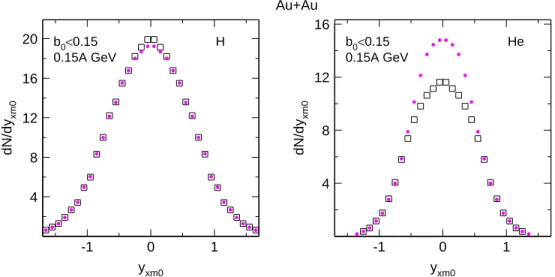
4.5 Z-renormalization

By Z-renormalization we address the sum-of-isotopes check and correction after 4π recon-struction, which uses the fact, shown earlier, that we had a more complete acceptance for fragments identified by charge only. This was most important for the low energy runs. We illustrate the necessary ’renormalization’ in Fig. 10 for hydrogen and helium isotopes in central collisions of Au+Au at 0.15A GeV. While renormalization is seen to be only a small effect for hydrogen, the worst case scenario shown for helium requires a significant correction for low transverse velocities, which can be traced back to errors due to not

-1.0 -0.5 0.0 0.5 1.0 y₀ 0.4 0.8 1.2 ut0 -1.0 -0.5 0.0 0.5 1.0 Au+Au 0.09A GeV

0.4 0.8 1.2 ut0 -1.0 -0.5 0.0 0.5 1.0 y₀ 0.4 0.8 1.2 ut0 -1.0 -0.5 0.0 0.5 1.0 Au+Au 0.25A GeV

0.4 0.8 1.2

ut0

Fig. 6. Example of 4π reconstruction of the phase space population for Z = 3 fragments in central (b0 < 0.15) Au+Au collisions at two indicated incident energies. The upper two panels show the measured part after applying some smoothing, a sharp filter cut and reflection symmetry, the lower two panels show the result of a two-dimensional extrapolation to 4π geometry.

protons 1 2 3 Ek₀ 104 105 dN/dp3 protons 1 2 3 Ek₀ Au+Au 0.4A GeV b₀<0.15

Fig. 7. Left panel: kinetic energies (scaled units) of protons emitted at 90◦

in central collisions of Au+Au. Comparison of two experiments performed in the low energy (full black circles) and the high energy campaigns (red squares). In the right panel the low energy experiment is rescaled along the abscissa by a factor 1.1 to achieve agreement with the high energy experiment.

accounting properly for Coulomb repulsion effects on low momenta not covered by our data.

-1.5 -1.0 -0.5 0.0 0.5 1.0 1.5 y_x0 1 2 3 dN/dy x0 -1.5 -1.0 -0.5 0.0 0.5 1.0 1.5 y_x0

Au+Au 0.4A GeV b₀<0.15 triton

Fig. 8. Sharp filtered transverse rapidity distributions for tritons in central Au+Au collisions at E/A = 0.4A GeV. Comparison of two experiments performed in the high energy (open red squares) and the low energy campaigns (full black circles). Left panel: original data. Right panel with the low energy data rescaled by factor 1.1 along the abscissa.

● FOPI ❑ Poggi 95 Au+Au protons b₀< 0.25 ERAT 10-1 100

beam energy (A GeV) 0.5 1.0 1.5 2.0 Ek0 /A

Fig. 9. Average kinetic energy (scaled units) of protons emitted around 90◦

(c.m.) in central col-lisions of Au+Au as a function of incident beam energy. The straight line fitted to the combina-tion of the low/high energy data (logarithmic abscissa) reproduces, after correction of the low energy data, the individual points with an av-erage accuracy of 1.2%. The data of [42] (red squares) are also shown.

5 Rapidity distributions

We present the phase space distributions in a way which deviates somewhat from the tra-ditional way: instead of showing standard (longitudinal) rapidity distributions on a linear ordinate scale and then switching for the transverse direction to transverse momentum distributions on a logarithmic scale, we show the transverse degree of freedom in the same representation as the longitudinal degree of freedom, namely in terms of transverse rapidi-ties plotted on a linear scale as well (see definitions in section 3). This allows to compare more directly longitudinal and transverse directions, a recurrent theme in the present work which is much concerned with assessing the degree of stopping and equilibration in these complex central collisions. We shall also be interested in the constrained transverse rapidity distributions (defined in section 3) which are likely to be closest to thermalized distributions.

b₀<0.15 0.15A GeV H -1 0 1 y_xm0 4 8 12 16 20 dN/dy xm0 b₀<0.15 0.15A GeV He -1 0 1 y_xm0 4 8 12 16 dN/dy xm0 Au+Au

Fig. 10. Left panel: Constrained transverse rapidity distribution of H fragments in central Au+Au collisions. (Black) open squares: demanding Z identification only, (pink) closed circles: sum of identified isotopes (p, d, t). Right panel: same for He.

been reconstructed using four different centralities in 25 system energies, i.e. 500 2d-spectra are available. This number could be doubled if we consider that two different selection criteria (ERAT and MUL, see section 3) were applied throughout. However, unless otherwise stated, we shall show generally only the ERAT selected data. Further, for E/A ≤ 0.4 GeV we have the data for heavier charge separated clusters (typically up to Z=8) and for E/A ≥ 0.4 GeV charged pion data of both polarities (see [38]). It is out of question to present here all this rich information. Instead we shall present samples which serve to illustrate some of the typical aspects of the LCP data and add a few remarks on heavier clusters and pion data [38]. In later sections some of these aspects will be summarized in terms of simple concepts: ’stopping’, ’radial flow’ and ’chemistry’. These concepts reflect the time sequence of the central reactions. Earlier work on these aspects will be referred to.

Some of the rapidity distributions will be compared with distributions expected from a Boltzmann thermal model. These thermal distributions are generated varying T until the variance of the constrained transverse rapidity distribution (i.e. with the scaled longi-tudinal distribution constrained by |yz0| < 0.5 and within the yxm0 range shown in the respective panels) is reproduced (the same constraints are used on the thermal simulation). The obtained T will be dubbed ’equivalent’ temperatures, Teq. The longitudinal constraint leads to a cutoff of part of the yields, a cutoff which is particle-mass and T dependent. This cut is corrected for when extracting so called effective ’mid-rapidity yields’ from the experimental data by comparison to the thermal model (see section 8).

5.1 Light charged particles (LCP)

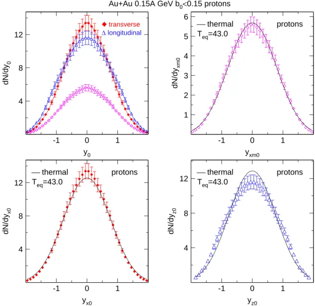
The next two 4-panel figures, Figs. 11, 12, show the three kinds of rapidity distributions for protons emitted in the most central Au+Au collisions at two incident energies differing by one order of magnitude: 0.15A GeV and 1.5A GeV.

 thermal T_eq=43.0 protons -1 0 1 y_x0 4 8 12 dN/dy x0 ◆ transverse ∆ longitudinal -1 0 1 y₀ 4 8 12 dN/dy 0  thermal T_eq=43.0 protons -1 0 1 y_z0 4 8 12 dN/dy z0  thermal T_eq=43.0 protons -1 0 1 y_xm0 1 2 3 4 5 6 dN/dy xm0

Au+Au 0.15A GeV b₀<0.15 protons

Fig. 11. Upper left panel: Longitudinal (blue open triangles) and transverse rapidity distribu-tions (red full diamonds) of protons in central collisions of Au+Au at 0.15A GeV beam energy. The third, lower yield curve (magenta open diamonds) in the panel represents the ’constrained’ transverse rapidity distribution: here a cut |yz0| < 0.5 on the longitudinal rapidity is applied. The smooth curves are just guides for the eye here. In the other three panels the three kinds of distributions are compared to a thermal distribution (corresponding to an equivalent tempera-ture of 43 MeV) having the same area as the respective data, but a variance as implied by the constrained transverse distribution (seen in upper right panel).

The upper-left panels in the two figures show that the longitudinal rapidity distributions are broader than the transverse distributions, but while the effect is relatively modest at the lower energy, it is more conspicuous at the higher energy. The constrained transverse distributions are generally somewhat broader than the integrated transverse distributions and can be reproduced rather well by a thermal model simulation having an adjusted ’equivalent’ temperature, Teq, and the same total area. We find Teq = 43 MeV, and 158 MeV, respectively, for protons at the two energies. This Teq comes closest to the ’inverse slopes’ usually fitted to pt spectra in the literature, but is different in the sense that it is

thermal T_eq=158 protons -1 0 1 y_x0 20 40 60 80 100 dN/dy x0 ◆ transverse ∆ longitudinal -1.5 -1.0 -0.5 0.0 0.5 1.0 1.5 y₀ 20 40 60 80 100 dN/dy 0 thermal T_eq=158 protons -1 0 1 y_z0 20 40 60 80 dN/dy z0 thermal T_eq=158 protons -1 0 1 y_xm0 10 20 30 40 50 dN/dy xm0

Au+Au 1.5A GeV b₀<0.15 protons

Fig. 12. Upper left panel: Longitudinal (blue open triangles) and transverse rapidity distribu-tions (red full diamonds) of protons in central collisions of Au+Au at 1.5A GeV beam energy. The ’constrained’ transverse rapidity distribution is also shown: here a cut |yz0| < 0.5 on the longitudinal rapidity is applied. The data points are joined by smooth curves to guide the eye. In the other three panels the three kinds of experimental distributions are compared to a thermal distribution (smooth black curves) having the same area as the respective data and a variance as implied by the constrained transverse distribution (seen in upper right panel).

obtained by just demanding a reproduction of the bulk experimental variances taken in the shown rapidity ranges and hence excluding far out tails of the distributions. On the

linear scales applied in the figures one finds a very satisfactory reproduction of the shape of

the dN/dyxm0 distributions (upper right panels). A comparison to the equivalent thermal representations fixed from the constrained data, to the full transverse and longitudinal distributions in the lower panels stresses the differences to the naive thermal expecta-tions. The full transverse distributions are modestly narrower only, but the longitudinal distributions clearly deviate.

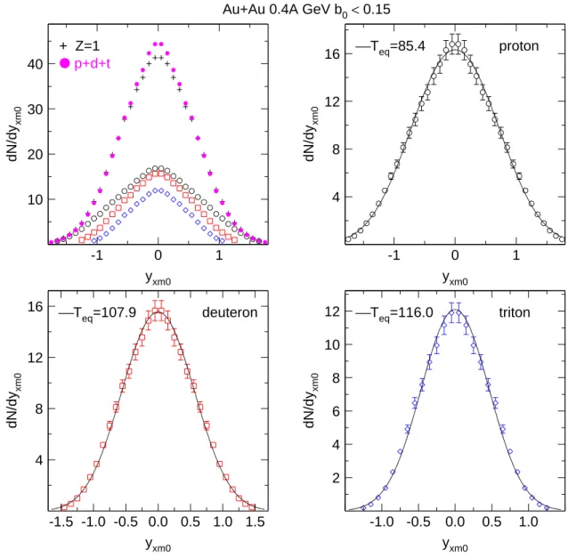
deuteron T_eq=107.9 -1.5 -1.0 -0.5 0.0 0.5 1.0 1.5 y_xm0 4 8 12 16 dN/dy xm0 + Z=1 ● p+d+t -1 0 1 y_xm0 10 20 30 40 dN/dy xm0 triton T_eq=116.0 -1.0 -0.5 0.0 0.5 1.0 y_xm0 2 4 6 8 10 12 dN/dy xm0 proton T_eq=85.4 -1 0 1 y_xm0 4 8 12 16 dN/dy xm0

Au+Au 0.4A GeV b₀< 0.15

Fig. 13. Central (b0< 0.15) Au+Au collisions at 0.4A GeV. Comparison of experimental scaled and constrained transverse rapidity distributions dN/dyxm0 of protons (upper right), deuterons (lower left) and tritons (lower right) with thermal distributions (smooth black curves) assuming the indicated equivalent temperatures Teq. The upper left panel shows the distributions of the three H isotopes, their sum (pink full dots) and the distribution for Z=1 (excluding created particles) obtained requiring only charge identification.

The next two 4-panel figures, Figs. 13, 14, take a closer look at constrained transverse rapidities varying the (hydrogen) isotope mass. The system is Au+Au at 0.4A GeV with b0 < 0.15. First we show the data, then a simulation with IQMD. In each case we make in the upper left panel the sum-of-isotopes check (which is fulfilled by definition in the simulation) and we compare in the other panels with a thermal model calculation adjusting Teq. These one-shape parameter fits are close to perfect, but require a rising equivalent temperature with the isotope mass, a well known phenomenon often interpreted as ’radial flow’ in the literature that we shall come back to in section 7. Clearly there is no global equilibrium, but at very best a ’local’ equilibrium (in the hydrodynamic sense).

T_eq=94.6 MeV IQMD-SM deuteron -1.5 -1.0 -0.5 0.0 0.5 1.0 1.5 y_xm0 2 4 6 8 10 dN/dy xm0 ◆ Z=1 -1 0 1 y_xm0 10 20 30 40 50 dN/dy T_eq=118 MeV IQMD-SM triton -1.0 -0.5 0.0 0.5 1.0 y_xm0 0.4 0.8 1.2 1.6 2.0 2.4 dN/dy xm0 T_eq=66.8 MeV IQMD-SM proton -1 0 1 y_xm0 10 20 30 40 dN/dy xm0

Au+Au 0.4A GeV b₀<0.15

Fig. 14. Central (b0 < 0.15) Au+Au collisions at 0.4A GeV. Comparison of simulated (IQMD-SM) scaled and constrained transverse rapidity distributions dN/dyxm0 of protons (up-per right), deuterons (lower left) and tritons (lower right) with thermal distributions (smooth black curves) assuming the indicated equivalent temperatures Teq.

A closer look at the simulated data reveals small but systematic shape differences that exceed those found when using experimental data instead of the IQMD events. One could argue that the experimental data look more ’thermal’. Note the rather strong decrease of yields with isotope mass in contrast to the more comparable yields in the experiment shown in the previous figure. Also, if one were to associate, naively, the strength of radial flow with the mass dependence of Teq, then one would conclude that the simulation overestimates the flow somewhat, since, as indicated in the various panels the Teq rise from 85 MeV for protons to 116 MeV for tritons in the data, while for the simulation we find 67 MeV and 118 MeV, respectively. For further discussions of the Teq values, see later section 7. The Fig. 15 showing constrained transverse rapidity distributions for central collisions in

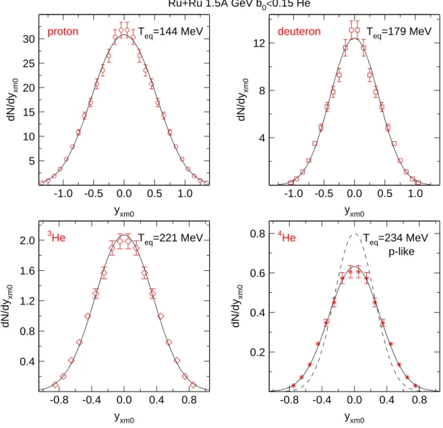
3 He T_eq=221 MeV -0.8 -0.4 0.0 0.4 0.8 y_xm0 0.4 0.8 1.2 1.6 2.0 dN/dy xm0 proton T_eq=144 MeV -1.0 -0.5 0.0 0.5 1.0 y_xm0 5 10 15 20 25 30 dN/dy xm0 4 He T_eq=234 MeV p-like -0.8 -0.4 0.0 0.4 0.8 y_xm0 0.2 0.4 0.6 0.8 dN/dy xm0 deuteron T_eq=179 MeV -1.0 -0.5 0.0 0.5 1.0 y_xm0 4 8 12 dN/dy xm0

Ru+Ru 1.5A GeV b₀<0.15 He

Fig. 15. Comparison of experimental constrained transverse rapidity distributions dN/dyxm0 with thermal distributions (black smooth curves) having the same first and second moments in central collisions of Ru+Ru at 1.5A GeV. The various ejectiles and the equivalent temperatures Teq are indicated. In the lower right panel we also plotted the4He distribution (dashed smooth curve, ’p-like’) expected if the equivalent temperature was the same as for protons, but with the integrated yields unchanged.

the system Ru+Ru at 1.5A GeV serves two purposes: 1) besides hydrogen isotopes (p and d) it also shows data for3_{He and}4_{He in the lower panels. Again thermal model calculations} with the indicated Teq are shown along with the data; 2) We show that the 4He data are not well represented by a coalescence model using the measured proton data as generating spectrum: see the dashed curve. Indeed the observed rising equivalent temperatures with mass contradict the naive model. This is at variance with ref. [43] where the validity of the power law for a wide range of incident energies and centralities in Au+Au systems was stressed. The authors mentioned that a cutoff of pt/A smaller than 0.2 GeV/c was required and that the single (’free’) proton spectra had to be used, rather than the total

3 He  T_eq=136.3 b₀<0.15 -1.0 -0.5 0.0 0.5 1.0 y_xm0 1 2 3 4 5 dn/dy xm0 3 He  T_eq=89.3 0.45<b₀<0.55 -1.0 -0.5 0.0 0.5 1.0 y_xm0 0.5 1.0 1.5 2.0 2.5 3.0 dn/dy xm0  T_eq=125.3 b₀<0.15 4 He -1.0 -0.5 0.0 0.5 1.0 y_xm0 2 4 6 8 10 dn/dy xm0  T_eq=81.2 0.45<b₀<0.55 4 He -1.0 -0.5 0.0 0.5 1.0 y_xm0 1 2 3 4 dn/dy xm0

Au+Au 0.4A GeV

Fig. 16. Central (b0 < 0.15) (bottom) and semi-central (top) Au+Au collisions at 0.4A GeV. Comparison of experimental scaled and constrained transverse rapidity distributions dN/dyxm0of 3_{He (left) and}4_{He (right) fragments with thermal distributions (smooth black curves) assuming} the indicated equivalent temperatures Teq.

spectra including those bound in clusters as one would naively expect. Non-perturbative features of clusterization are suggested strongly by our data, as we shall show later in this section and in section 8.

In the cases shown so far we observe a regular rise of Teq with the mass of the ejectile. However, frequently in the literature, the so-called ’helium anomaly’ is mentioned [44], namely the observation that 3_{He kinetic energies are not lower, but higher than the} 4_He energies, a phenomenon that to our knowledge has not been reproduced by microscopic dynamic reaction models. In Fig. 16 we show for Au+Au that even at the relatively high incident energy of E/A = 0.4 GeV this phenomenon still subsists to some degree as the Teq for4He are not found to exceed those of 3He. Further we show in the panels the rather

protons

❍ IQMD-SM

◆ FOPI

-1 0 1

y_xm0

Au+Au 0.4A GeV b₀<0.15

100 101 102 dN/dy xm0 ◊3 H ◆3He -1.0 -0.5 0.0 0.5 1.0 y_xm0

Au+Au 0.4A GeV b₀<0.15

10-1 100 101

dN/dy

xm0

Fig. 17. Left panel: Constrained transverse rapidity distributions of protons in central collisions of Au+Au. Comparison of data (red closed diamonds) and IQMD simulation (blue open circles). Right panel: comparison of experimental data for 3_{He (red closed diamonds) and}3_{H (blue open} diamonds) in the same reaction.

strong drop of Teq with decreasing centrality, which is varied from b0 < 0.15 (lower panels) to 0.45 < b0 < 0.55 (upper panels). This is a general feature also observed at other energies and was reported earlier [45].

5.2 The influence of clusterization

The failure of the naive coalescence approach consisting in trying to reproduce the spectra of heavier clusters from the measured nucleon (proton) spectra (Fig. 15) and some of the ’He-anomaly’ discussed before may be connected with our current failure to understand clusterization quantitatively on a microscopic level (compare also the upper right panels of Figs. 13 and 14). Concerning the probability of nucleons to cluster, we are at SIS in a non-perturbative regime (see section 8): heavier cluster formation has a back-influence on the lighter generating transverse rapidity spectra.

The two-panel Fig. 17 illustrates the non-perturbative features at SIS. In the left panel we show the remarkable difference between FOPI and IQMD for the transverse rapidity distributions of protons. The surplus of IQMD for lower transverse velocities or momenta is due to a lack of sufficient clusterization: in the experiment more copious cluster for-mation massively depletes the low momenta. The right panel compares two experimental distributions: now it is the 3_{He that appears to have its low momenta depleted relative} to3_{H (the naive perturbative coalescence model does not predict any difference here). In} view of the finding of the left panel, it is tempting to associate the effect to the formation of heavier clusters from the ’primeval’ 3_{He (created in earlier expansion stages).}

to-❑3 H-3He ●4 He x 1.2 -1.0 -0.5 0.0 0.5 1.0 y_xm0

Au+Au 0.4A GeV b₀<0.15

2 4 6 8

dN/dy

xm0 Fig. 18. Comparison of the difference

spec-trum (see right panel previous figure) 3_H-3_He (rescaled by a factor 1.2) to the4_{He (black dots)} transverse rapidity spectrum.

gether with data for 4_{He. The}3_{H and the} 3_{He compete to be a condensation nucleus to a} possible4_{He. If both mass 3 isotopes are in a neutron-rich environment, the}3_{He will ’win’} for two reasons:

a) it is easier to ’find’ a single neutron to attach to 3_{He than a single proton to attach to} 3_H;

b) in contrast to 3_{H, the} 3_{He nucleus does not Coulomb-repulse its needed partner.} A quantitative transport model theory must include the formation of α clusters if these conjectures are correct.

5.3 How to define stopping: varxz

The final figure in this section on rapidity distributions, Fig. 19, serves to illustrate what we shall call ’partial transparency’ or ’incomplete stopping’. Transparency increases as either the studied system mass is lowered, or the incident energy is raised by going from E/A = 0.4 GeV (lower panels) to 1.5 GeV (upper panels). With this figure, which shows data for the most central collisions (b0 < 0.15 or 2.2% of the equivalent sharp cross section), we argue that a good measure of the degree of stopping consists in evaluating the ratio varxz of variances varx and varz of the transverse relative to the longitudinal rapidity distribution, respectively, both of which are shown in the figure for deuterons. Note also the subtle evolution of shapes, especially at the higher energy: there is no trivial subdivision into ’participants’ or ’spectators’ possible. The interpretation in terms of two remnant counterflowing (not completely stopped) ’fluids’ is strongly supported by isospin tracer methods (see section 6) and suggests that not only global, but also local equilibrium is not achieved.

◆ transverse ∆ longitudinal Ca+Ca varxz 0.402 -1.5 -1.0 -0.5 0.0 0.5 1.0 1.5 y₀ 0.4A GeV b₀<0.15 2 4 6 8 ◆ transverse ∆ longitudinal Ca+Ca varxz 0.247 -1.5 -1.0 -0.5 0.0 0.5 1.0 1.5 y0 1.5A GeV b0<0.15 2 4 6 8 10 12 ◆ transverse ∆ longitudinal Ru+Ru varxz 0.676 -1.5 -1.0 -0.5 0.0 0.5 1.0 1.5 y₀ 0.4A GeV b₀<0.15 4 8 12 16 ◆ transverse ∆ longitudinal Ru+Ru varxz 0.418 -1.5 -1.0 -0.5 0.0 0.5 1.0 1.5 y0 1.5A GeV b0<0.15 5 10 15 20 25 ◆ transverse ∆ longitudinal Au+Au varxz 0.913 -1.5 -1.0 -0.5 0.0 0.5 1.0 1.5 y₀ 0.4A GeV b₀<0.15 5 10 15 20 25 ◆ transverse ∆ longitudinal Au+Au varxz .458 -1.5 -1.0 -0.5 0.0 0.5 1.0 1.5 y0 1.5A GeV b0<0.15 10 20 30 40 50 dN/dy 0

Fig. 19. Comparison of scaled rapidity distributions for deuterons in central collisions at E/A = 1.5 GeV (top panels) and 0.4 GeV (bottom panels): shown are data for Ca+Ca, Ru+Ru and Au+Au (from left to right). In each panel, the scaled longitudinal rapidity yz0distributions (blue open triangles) are shown together with the scaled transverse rapidity yx0 distributions (red). The derived value of the stopping observable varxz is also indicated.

6 Stopping

As introduced in section 5.3, we quantify the degree of stopping by comparing the variances of transverse rapidity distributions (defined in section 3) with that in the longitudinal (z) direction. Throughout we use scaled rapidities (i.e. the rapidity gap is projected unto the fixed interval (−1, +1)) and typical samples have been shown and discussed already (sec-tion 5). All rapidities are evaluated in the c.m.. However, for the ratios we discuss the scaling is immaterial. We shall call varxz the ratio of the variances in the x-direction and the z direction. The choice of x is arbitrary, i.e. it is not connected with the azimuth of the reaction plane. varxz(1) is defined like varxz except that the integrations for calculating the variance are limited to the range |yz0| < 1; in [32] this was called vartl and |yx0| was also constrained to be < 1. Such a restricted measure of stopping can be more adequate if measured data outside the range |yz0| < 1 are missing or less reliable. For varxz(0.5) the transverse rapidity distribution is taken under the constraint |yz0| < 0.5 on the scaled

longitudinal rapidity. This measure of stopping is clearly biased and has systematically

higher values, but is of interest when comparing with many data in the (higher energy) literature, where often attention is focused on transverse momentum spectra around (lon-gitudinal) midrapidity. When no number in parenthesis is given, the intervals in rapidity are sufficiently broad to make the value of varxz asymptotically stable within the indicated, mostly systematic, errors.

There are other ways of characterizing stopping. Videbaek and Hansen [46] have introduced the mean rapidity shift < δy > which is defined by

< δy >≡

Rycm

−∞ |y − ytgt|(dNp/dy)dy

Rycm

−∞(dNp/dy)dy

where ycm is the rapidity of the c.m., ytgt is the target rapidity and dNp/dy is the proton rapidity distribution (a similar formula exists relative to the projectile rapidity yp with the integration limits interchanged). This observable was also determined in some works of our Collaboration, [48,49]. The inelasticity K was used by NA49 [47] and is defined by K = Einel/(√s/2 − mp) with Einel being equal to the average energy loss of incident nucleons with rest mass mp. The common feature of these definitions is that one assesses stopping relative to initial conditions: the conclusion is then that a high degree of stopping is reached in collisions all the way up to at least SPS energies, especially if it is assessed in terms of energies. Our stopping variable has a different goal: we want to assess the difference relative to a completely stopped scenario, an assumption that is frequently assumed in (one-fluid) hydrodynamic codes for heavy ion collisions because of its inherent simplicity of a needed starting point of the calculation. Our observable, varxz, is important to assess the partial memory of the original (accelerator induced) counterflow of two fluids and hence deviations from local equilibrium. It is also of value to help determine viscosity properties of nuclear matter [50].

6.1 Isospin tracing

We invariably find that longitudinal rapidity distributions are broader than transverse rapidity distributions, see section 5. In principle, for a given system, one cannot exclude that this phenomenon is caused by a rebound opposite to the incident direction after a complete stop. The system size dependence of the effect, see namely Fig. 19, can be used to strongly argue against this interpretation which would imply an unlikely stronger rebound in smaller systems. An alternative method to demonstrate partial transparency was introduced by our Collaboration [52] and consists in so called isospin tracing. We refer the reader to the original publication for further explanations. Briefly, we combine rapidity distribution information of four systems involving the isotopes 96_{Zr and} 96_{Ru : Ru+Ru,} Zr+Zr, Ru+Zr and Zr+Ru, where the mixed systems are merely technically different in the sense that beam and target are inverted.

In the following, abbreviating NRuZr

y (p) the rapidity distribution of protons in the reaction Ru+Zr, etc, we define

R4y(p) = [NyRuZr(p) − NyZrRu(p)]/[NyRuRu(p) − NyZrZr(p)]

This observable is a slight variant of the observable RZ used in [52]: it is an average of the two opposite-sign branches obtained by switching target and projectile in the mixed system. An arbitrary (here negative) equal sign is defined (the two branches of RZ in the chosen symmetric-mass systems must be equal except for sign). In Fig. 20 we show R4y for central collisions at 0.4A and 1.5A GeV together with rapidity distribution plots. In case of complete mixing with loss of memory (both alternatives: rebound as well as partial

0.4A GeV ❑ b₀< 0.15 ∆ b₀< 0.25 -1.0 -0.5 0.0 y_z0 -1.0 -0.5 0.0 R4y ◆ transverse ∆ longitudinal Ru+Ru 0.4A GeV b0<0.15 -2 -1 0 1 2 y₀ 4 8 12 16 20 24 dN/dy 0 ❑ b₀< 0.15 ∆ b₀< 0.25 1.5A GeV -1.0 -0.5 0.0 y_z0 -1.0 -0.5 0.0 R4y ◆ transverse ∆ longitudinal Ru+Ru 1.5A GeV b0<0.15 -1 0 1 y₀ 10 20 30 40 50 60 dN/dy 0

Fig. 20. Top panels: Longitudinal and transverse rapidity distributions of protons in collisions of Ru+Ru at 0.4A GeV (left) and 1.5A GeV. Bottom panels: The corresponding R4y observables for two slightly different indicated centralities as a function of the longitudinal rapidity yz0. transparency) of the incident geometry, the rapidity dependences of R4y should be flat at zero value. There is indeed a small flat part around yz0= 0, especially for the most central (b0 < 0.15) selection, but for higher |yz0| there is an increasing deviation from zero, the sign of which can be unambiguously associated with transparency, rather than rebound. The effect is definitely more pronounced at the higher energy in full accordance with the information from the variances of the rapidity distributions (see the upper panels in the figure). Only statistical errors are shown in the lower panels of Fig. 20. A more detailed presentation and discussion of the new isospin tracing data will be published elsewhere [53].

6.2 Global stopping and the EOS

By adding up the measured rapidity distributions of the different ejectiles one can try to obtain a global system stopping. The excitation function for Au on Au, first published in [32], was later slightly revised and combined with data from the INDRA collaboration

▼ HM ◆ SM ∆ FOPI ● INDRA ERAT b(0)< 0.15

10

10

beam energy (A GeV)

Au+Au

0.5

0.6

0.7

0.8

0.9

1.0

varxz(1)

Fig. 21. Excitation function of the stopping observable varxz(1) in central Au+Au collisions (b0 < 0.15) [32,33] . FOPI data: open blue triangles, INDRA data: black dots. These experimental data points are joined by straight line segments to guide the eye. IQMD simulations extending from 0.12A to 1.5A GeV: red full triangles (HM) and green full diamonds (SM).

[33]. The combined data are shown again in Fig. 21, but this time together with IQMD simulations using alternatively a hard (K = 380 MeV, HM) or a soft (K = 200 MeV, SM) EOS with momentum dependence [7]. As can be seen from the Figure, the difference between the HM and the SM simulation is significantly larger than the error bars in the data. This is an important observation as it opens up the possibility to observe EOS sensitivity also in central collisions in contrast to directed and elliptic flow which are linked to off-centrality (and in general collisions with less achieved compression). However, it is also clear that the ’residual’ interaction, i.e. the explicit collision term, influences the outcome. The present parameterization of IQMD as used here is obviously not able to reproduce the data, in particular the rapid drop of varxz(1) beyond 0.8A GeV is not reproduced. A fair reproduction of a portion (0.25A to 1.0A GeV) of the excitation function was achieved in [50].

Clearly, varxz data should prove useful also to constrain the viscosity of nucleonic (and more generally of hadronic) matter if compared to transport model simulations. It is tempting to conjecture that the rising part of the excitation function is dominated by the decreasing importance of Pauli blocking as the rapidity gap exceeds the Fermi energy. Particle creation starts becoming important beyond 1A GeV [38] (see also our Fig.41 in the present work). But the decreasing trend of the varxz data seen in Fig. 21 suggests that this new channel does not compensate for the decrease and forward focusing of elastic nucleon-nucleon processes. The rapid decrease of varxz at the high SIS energy end is continued at AGS and SPS as we shall show later for net protons.

triton

0.4 0.8 1.2 1.6

beam energy (GeV) 0.4 0.5 0.6 0.7 0.8 0.9 1.0 varxz proton 0.4 0.5 0.6 0.7 0.8 0.9 1.0 varxz Z=1 0.4 0.8 1.2 1.6

beam energy (GeV) deuteron Au+Au b₀<0.15

Fig. 22. Excitation function of the stopping observable varxz in central Au+Au collisions (b0 < 0.15). As indicated in the various panels the excitation functions are shown separately for the three hydrogen isotopes. The right-lower panel allows to compare relative to the average weighted Z=1 fragments. The smooth curve is just a polynomial fit.

6.3 p, d, t stopping: a hierarchy

By plotting varxz separately for identified fragments further insights (and constraints to simulations) can be gained. This is shown in Fig. 22. A remarkable feature is the similarity in the behaviour for the three isotopes, that suggests the collectivity of the phenomenon. There is a well defined maximum around 0.4A GeV for each of the isotopes qualitatively similar to the observed [32] global stopping. On the other hand a closer look reveals that there are some subtle differences in the shapes of the excitation functions. Except around the maximum, there is a hierarchy in the degree of stopping. This is illustrated in Fig. 23. On the average clusters have ’seen’ less violent (less stopped) collisions when the stopping is incomplete for single emitted nucleons (away from the maximum around 0.4A GeV).

❑

varxz

∆

varxz(0.5)

0.80A GeV

1

2

3

0.5

0.6

0.7

0.8

0.9

1.0

1.1

❑

varxz

∆

varxz(0.5)

0.12A GeV

0.6

0.7

0.8

0.9

1.0

1.1

❑

varxz

∆

varxz(0.5)

1.20A GeV

1

2

3

0.4A GeV

❑

varxz

∆

varxz(0.5)

mass (u)

Au+Au p,d,t b

<

0.15

varxz

Fig. 23. Mass number dependence of the stopping observable varxz of hydrogen fragments in central Au+Au collisions (b0 < 0.15). Data are shown for 4 representative energies indicated in the panels (notice the one order of magnitude span). For comparison data are also shown for the ’constrained’ stopping observable varxz(0.5) (blue open triangles, error bars omitted). The lines are linear fits.

This effect may be a surface effect but is not a ’trivial’ spectator-matter effect, as the rapidity distributions in these most central collisions do not exhibit well defined ’spectator ears’ around |yz0| = 1: there are no spectators in the strict sense here. The constrained stopping varxz(0.5) (blue open triangles in the figure) is always somewhat larger because the transverse rapidity distributions are broadened when a cut around longitudinal rapidity is applied. The trends with mass number and incident energy are similar however.

6.4 System size dependence of stopping

As remarked earlier, the system size dependence of the observable varxz is an important constraint to the question of transparency versus rebound dominated collision scenario, es-pecially when only the most central collisions are compared in scaled units of centrality. All our data support transparency dominance. This does not mean that the degree of stopping is small, but it is significantly less than expected from ideal one-fluid hydrodynamics. Figure 24 shows a rather complex behaviour and will be a challenge to ambitious mi-croscopic simulations. One remarkable feature is the apparent saturation of varxz at a relatively low value for the highest incident energy. This was already seen earlier, [32], for global stopping. This suggests the beginning of a phenomenon seen in a more spectacular way recently at the SPS [47] (E/A = 158A GeV): at midrapidity there is no non-trivial increase of population in Pb+Pb relative to p+p collisions.

6.5 Isospin and stopping

One expects isospin dependences because the free nucleon-nucleon cross sections σnn and σnp are different and also because the mean fields, shown earlier to influence global stop-ping, are expected to be isospin dependent. However the data show no convincing effect considering the error limits. This is shown in Fig. 25 where a comparison of two sys-tems with the same mass, but different composition (Ru+Ru, N/Z = 1.182 and Zr+Zr, N/Z = 1.400) is shown. In this context it is interesting to note that very recently a similar observation was made [51] at lower energies (32 − 100A MeV) for Xe+Sn using various isotopes.

6.6 Centrality dependence of stopping

For comparisons with simulations it is useful to check how sensitively the observable varxz reacts to matching the centrality correctly with that of the experiment. The relatively strong dependence of varxz on centrality b0 is illustrated in Fig. 26 for Au+Au at two rather different incident energies. The linear fits allow to estimate a limit for b0 = 0. Since

varxz is the ratio of varx and varz (the zero suffix is immaterial here since the scaling

cancels out ), it is interesting to explore what causes the strong centrality dependence. The figure also illustrates the comparatively modest change of the scaled variance, varxm0 of the constrained transverse rapidity distribution (which we remind is obtained with a with a cut |yz0| < 0.5 on the scaled longitudinal rapidity).

6.7 Heavy clusters

Since at lower energies we have been able to get information also for fragments with Z > 2, we can extend the hierarchy of stopping to heavy clusters. The results are put together