Higher harmonic flow coefficients of identified hadrons in Pb-Pb collisions at $\sqrt{s_{\rm NN}}$ = 2.76 TeV

CERN-PH-EP-2016-159 15 June 2016

c

2016 CERN for the benefit of the ALICE Collaboration.

Reproduction of this article or parts of it is allowed as specified in the CC-BY-4.0 license.

Higher harmonic flow coefficients of identified hadrons in Pb–Pb

collisions at

√

s

= 2.76 TeV

ALICE Collaboration∗

Abstract

The elliptic, triangular, quadrangular and pentagonal anisotropic flow coefficients for π±, K±and

p+p in Pb–Pb collisions at√sNN= 2.76 TeV were measured with the ALICE detector at the Large

Hadron Collider. The results were obtained with the Scalar Product method, correlating the identified hadrons with reference particles from a different pseudorapidity region. Effects not related to the common event symmetry planes (non-flow) were estimated using correlations in pp collisions and were subtracted from the measurement. The obtained flow coefficients exhibit a clear mass ordering

for transverse momentum (pT) values below ≈ 3 GeV/c. In the intermediate pT region (3 < pT<

6 GeV/c), particles group at an approximate level according to the number of constituent quarks, suggesting that coalescence might be the relevant particle production mechanism in this region. The

results for pT< 3 GeV/c are described fairly well by a hydrodynamical model (iEBE-VISHNU)

that uses initial conditions generated by A Multi-Phase Transport model (AMPT) and describes the expansion of the fireball using a value of 0.08 for the ratio of shear viscosity to entropy density (η/s), coupled to a hadronic cascade model (UrQMD). Finally, expectations from AMPT alone fail to quantitatively describe the measurements for all harmonics throughout the measured transverse momentum region. However, the comparison to the AMPT model highlights the importance of the

late hadronic rescattering stage to the development of the observed mass ordering at low values of pT

and of coalescence as a particle production mechanism for the particle type grouping at intermediate

values of pTfor all harmonics.

∗_{See Appendix B for the list of collaboration members}

Contents

1 Introduction 3

2 Experimental setup 4

3 Event sample, track selection and particle identification 5

3.1 Trigger selection and data sample . . . 5

3.2 Track selection . . . 5

3.3 Identification of π±, K±and p+p . . . 6

4 Analysis technique 7 4.1 Scalar Product method . . . 7

4.2 Estimation of non-flow correlations . . . 7

5 Systematic uncertainties 8 6 Results and discussion 11 6.1 Centrality dependence of flow harmonics . . . 11

6.2 Evolution of flow harmonics in ultra-central Pb–Pb collisions . . . 15

6.3 Mass ordering . . . 15

6.4 Test of scaling properties . . . 18

6.5 Comparison with models . . . 19

6.5.1 Comparison with iEBE-VISHNU . . . 19

6.5.2 Comparison with AMPT . . . 20

7 Conclusions 22 A Additional figures 30 A.1 Integrated vn. . . 30

A.2 NCQ scaling . . . 30

A.3 KETscaling . . . 32

1 Introduction

Quantum chromodynamics (QCD) calculations on the lattice [1, 2] suggest that at high values of tem-perature and energy density a transition takes place from ordinary nuclear matter to a state where the constituents, the quarks and the gluons, are deconfined. This state of matter is called the quark-gluon plasma (QGP) [3–5]. The aim of the heavy-ion program at the Large Hadron Collider (LHC) is to study the QGP properties, such as the equation of state, the speed of sound in the medium, and the value of the ratio of shear viscosity to entropy density (η/s).

One of the important observables sensitive to the properties of the QGP is the azimuthal distribution of particles emitted in the plane transverse to the beam direction. In non-central collisions between two heavy ions the overlap region is not isotropic. This spatial anisotropy of the overlap region is transformed into an anisotropy in momentum space initially through interactions between partons and at later stages between the produced particles. The resulting anisotropy is usually expressed in terms of a Fourier series in azimuthal angle ϕ [6, 7] according to

Ed 3_N dp3 = 1 2π d2N pTdpTdη n 1 + 2 ∞

∑

where E, N, p, pT, ϕ and η are the energy, particle yield, total momentum, transverse momentum,

azimuthal angle and pseudorapidity of particles, respectively, and Ψnis the azimuthal angle of the

sym-metry plane of the nth-order harmonic [8–11]. The nth-order flow coefficients are denoted as vn and can

be calculated as

vn= hcos[n(ϕ − Ψn)]i, (2)

where the brackets denote an average over all particles in all events. Since the symmetry planes are not accessible experimentally, the flow coefficients are estimated solely from the azimuthal angles of the produced particles. The second Fourier coefficient, v2, measures the elliptic flow, i.e. the momentum

space azimuthal anisotropy of particle emission relative to the second harmonic symmetry plane. The study of v2 at both the Relativistic Heavy Ion Collider (RHIC) and the LHC contributed significantly

to the realisation that the produced system can be described as a strongly-coupled quark-gluon plasma (sQGP) with a small value of η/s, very close to the conjectured lower limit of 1/4π from AdS/CFT [12]. In addition, the overlap region of the colliding nuclei exhibits an irregular shape [8–11, 13]. The irreg-ularities originate from the initial density profile of nucleons participating in the collision, which is not isotropic and differs from one event to the other. This, in turn, causes the symmetry plane of the irregular shape to fluctuate in every event around the reaction plane, defined by the impact parameter vector and the beam axis, and also gives rise to the additional higher harmonic symmetry planes Ψn. The initial

state fluctuations yield higher order flow harmonics such as v3, v4, and v5 that are usually referred to

as triangular, quadrangular, and pentagonal flow, respectively. Recent calculations [14, 15] suggest that their transverse momentum dependence is a more sensitive probe than elliptic flow not only of the initial geometry and its fluctuations, but also of η/s. The first measurements of the pT-differential vn, denoted

as vn(pT), of charged particles at the LHC [16–18] provided a strong testing ground for

hydrodynam-ical calculations that attempt to describe the dynamhydrodynam-ical evolution of the system created in heavy-ion collisions.

An additional challenge for hydrodynamical calculations and a constraint on both the initial conditions and η/s can be provided by studying the flow coefficients of Eq. 2 as a function of collision centrality and transverse momentum for different particle species. The first results of such studies at RHIC [19–22] and the LHC [23, 24] revealed that an interplay of radial flow (the average velocity of the system’s collective

radial expansion) and anisotropic flow leads to a characteristic mass dependence of v2(pT) [25–27] for

pT < 3 GeV/c. For higher values of transverse momentum up to pT ≈ 6 GeV/c these results indicate

that the v2of baryons is larger than that of mesons. This behaviour was explained in a dynamical model

where flow develops at the partonic level followed by quark coalescence into hadrons [28, 29]. This mechanism leads to the observed hierarchy in the values of v2(pT), referred to as number of constituent

quarks (NCQ) scaling. New results from ALICE [23] and PHENIX [30] exhibit deviations from the NCQ scaling at the level of ±20% for pT> 3 GeV/c. In addition, the LHC results showed also that the v2 of

the φ -meson at intermediate values of transverse momentum follows the baryon rather than the meson scaling for central Pb–Pb collisions [23]. Recently, the first results of v2(pT), v3(pT), and v4(pT) for π±,

K±and p+p for 50% most central Au–Au collisions at√s_NN= 200 GeV were reported [31]. The higher harmonic flow coefficients exhibit similar mass and particle-type dependences as v2 up to intermediate

values of pT.

In this article, we report the results for the pT-differential elliptic, triangular, quadrangular and pentagonal

flow for π±, K± and p+p measured in Pb–Pb collisions at the centre of mass energy per nucleon pair √

sNN= 2.76 TeV with the ALICE detector [32, 33] at the LHC. The particles are identified using signals

from both the Time Projection Chamber (TPC) and the Time Of Flight (TOF) detectors, described in Section 2, with a procedure that is discussed in Section 3. The results are obtained with the Scalar Product method described in Section 4, and in detail in Refs. [23, 34–36]. In this article, the identified hadron under study and the charged reference particles are obtained from different, non-overlapping pseudorapidity regions. A correction for correlations not related to the common symmetry plane (non-flow), like those arising from jets, resonance decays and quantum statistics correlations, is presented in Section 4. This procedure relies on measuring the corresponding correlations in pp collisions and subtracting them from the vn coefficients measured in Pb–Pb collisions to form the reported vsubn (pT),

where the superscript ‘sub’ is used to stress the subtraction procedure. The systematic uncertainties of the measurements are described in Section 5. All harmonics were measured separately for particles and anti-particles and were found to be compatible within the statistical uncertainties. Therefore, the vsub_n (pT)

for the average of the results for the opposite charges is reported. The results are reported in Section 6 for the 0–50% centrality range of Pb–Pb collisions. Finally, results are also reported separately for ultra-central events, i.e. the 0–1% ultra-centrality range, where the role of the collision geometry is reduced and one expects that vsubn (pT) is mainly driven by the initial state fluctuations.

2 Experimental setup

ALICE [32, 33] is one of the four large experiments at the LHC, particularly designed to cope with the large charged-particle densities present in central Pb–Pb collisions [37]. By convention, the beam direction defines the z-axis, the x-axis is horizontal and points towards the centre of the LHC, and the y-axis is vertical and points upwards. The apparatus consists of a set of detectors located in the central barrel, positioned inside a solenoidal magnet which generates a 0.5 T field parallel to the beam direction, and a set of forward detectors.

The Inner Tracking System (ITS) [32] and the TPC [38] are the main tracking detectors of the central barrel. The ITS consists of six layers of silicon detectors employing three different technologies. The two innermost layers, positioned at r = 3.9 cm and 7.6 cm, are Silicon Pixel Detectors (SPD), followed by two layers of Silicon Drift Detectors (SDD) (r = 15 cm and 23.9 cm). Finally, the two outermost layers are double-sided Silicon Strip Detectors (SSD) at r = 38 cm and 43 cm. The TPC surrounds the ITS and provides full azimuthal coverage in the pseudorapidity range |η| < 0.9.

Charged pions, kaons and protons were identified using the information from the TPC and the TOF de-tectors [32]. The TPC allows for a simultaneous measurement of the momentum of a particle and its specific energy loss hdE/dxi in the gas. The detector provides a separation by at least 2 standard

devia-tions for the hadron species at pT< 0.7 GeV/c and the possibility to identify particles in the relativistic

rise region of dE/dx (i.e. 2 < pT< 20 GeV/c) [33]. The dE/dx resolution for the 5% most central Pb–Pb

collisions is 6.5% and improves for more peripheral collisions. The TOF detector is placed around the TPC and provides a 3σ separation between π–K and K–p up to pT = 2.5 GeV/c and pT = 4 GeV/c,

respectively [33]. This is done by measuring the flight time of particles from the collision point with a resolution of about 80 ps. The start time for the TOF measurement is provided by the T0 detectors, two arrays of Cherenkov counters positioned at opposite sides of the interaction points covering 4.6 < η < 4.9 (T0A) and −3.3 < η < −3.0 (T0C). The start time is also determined using a combinatorial algorithm that compares the timestamps of particle hits measured by the TOF to the expected times of the tracks, assuming a common event time tev[33]. Both methods of estimating the start time are fully efficient for

the 50% most central Pb–Pb collisions.

A set of forward detectors, the V0 scintillator arrays [39], were used in the trigger logic and for the de-termination of the collision centrality, discussed in the next section. The V0 consists of two systems, the V0A and the V0C, that are positioned on each side of the interaction point and cover the pseudorapidity ranges of 2.8 < η < 5.1 and −3.7 < η < −1.7, respectively.

For more details on the ALICE experimental setup and the performance of the detectors, see Refs. [32, 33].

3 Event sample, track selection and particle identification

3.1 Trigger selection and data sample

The analysis is performed on data from pp and Pb–Pb collisions at√s_NN= 2.76 TeV collected with the ALICE detector in 2011. The minimum bias trigger in pp collisions required at least one hit in either of the V0 detectors or the SPD. In Pb–Pb collisions, minimum bias events were triggered by the coincidence between signals from the two sides of the V0 detector. In addition, in Pb–Pb collisions, an online selec-tion based on the V0 detectors was used to increase the number of central (i.e. 0–10% centrality range) and semi-central (i.e. 10–50% centrality range) events. An offline event selection, exploiting the signal arrival time in V0A and V0C, measured with a 1 ns resolution, was used to discriminate background (e.g. beam–gas) from collision events. This led to a reduction of background events in the analysed samples to a negligible fraction (< 0.1%) [33]. All events selected for the analysis had a reconstructed primary vertex position along the beam axis (zvtx) within 10 cm from the nominal interaction point.

Fi-nally, events with multiple reconstructed vertices were rejected, leading to a negligible amount of pile–up events for all systems [33]. After all the selection criteria, a filtered data sample of approximately 25 × 106Pb–Pb and 20 × 106pp events were analysed to produce the results presented in this article. Events were classified according to fractions of the inelastic cross section and correspond to the 50% most central Pb–Pb collisions. The 0–1% interval represents the most central interactions (i.e. smallest impact parameter) and will be referred to as ultra-central collisions in the following. On the other hand, the 40–50% interval corresponds to the most peripheral (i.e. largest impact parameter) collisions in the analysed sample, imposed by the usage of the semi-central trigger for the collected sample in 2011. The centrality of the collision was estimated using the distribution of signal amplitudes from the V0 detectors. The systematic uncertainty due to the centrality estimation is determined using the charged particle mul-tiplicity distribution of TPC tracks and the number of SPD clusters, and will be discussed in Section 5. Details about the centrality determination can be found in Ref. [40].

3.2 Track selection

In this analysis, tracks are reconstructed using the information from the TPC and the ITS detectors. The tracking algorithm, based on the Kalman filter [41, 42], starts from a collection of space points (referred to as clusters) inside the TPC, and provides the quality of the fit by calculating its χ2 value. Each

space point is reconstructed at one of the TPC padrows, where the deposited ionisation energy is also measured. The specific ionisation energy loss hdE/dxi is estimated using a truncated mean, excluding the 40% highest-charge clusters associated to the track. The obtained hdE/dxi has a resolution, which we later refer to as σTPC. The tracks are propagated to the outer layer of the ITS, and the tracking

algorithm attempts to identify space points in each one of the consecutive layers, reaching the innermost ones (i.e. SPD). The track parameters are then updated using the combined information from both the TPC and the ITS detectors. If the algorithm is unable to match the track reconstructed in the TPC with associated ITS clusters (e.g. due to inefficiencies caused by dead channels in some of the ITS layers), the track parameters calculated from the TPC tracking algorithm are used instead. This tracking mode will be referred to as hybrid tracking in the rest of the text, and is used as the default in this analysis since it also provides uniform ϕ distribution.

Primary charged pions, kaons and (anti-)protons were required to have at least 70 reconstructed space points out of the maximum of 159 in the TPC. The average χ2 of the track fit per TPC space point per degree of freedom (see [33] for details) was required to be below 2. These selections reduce the con-tribution from short tracks, which are unlikely to originate from the primary vertex. To further reduce the contamination by secondary tracks from weak decays or from the interaction with the material, only particles within a maximum distance of closest approach (DCA) between the tracks and the primary ver-tex in both the transverse plane (DCAxy< 2.4 cm) and the longitudinal direction (DCAz< 3.2 cm) were

analysed. Moreover, the tracks were required to have at least two associated ITS clusters in addition to having a hit in either of the two SPD layers. This selection leads to an efficiency of about 80% for pri-mary tracks at pT> 0.6 GeV/c and a contamination from secondaries of about 5% at pT= 1 GeV/c [43].

These values depend on particle species and transverse momentum [43].

The systematic uncertainty due to the track reconstruction mode was estimated using two additional tracking modes, one relying on the so-called standalone TPC tracking with the same parameters de-scribed before, and a second that relies on the combination of the TPC and the ITS detectors (i.e. global tracking) with tighter selection criteria. In the latter case, the maximum value of DCA was 0.3 cm in both the transverse plane and the longitudinal direction, thus further reducing the amount of secondary particles in the track sample.

The results are reported for all identified hadrons in |η| < 0.8 and for the transverse momentum range 0.3 < pT< 6.0 GeV/c for π±and 0.3 < pT< 4.0 GeV/c for K±. Finally, since the contamination from

secondary protons created through the interaction of particles with the detector material can reach values larger than 5% for pT < 1 GeV/c, only p were considered for 0.4 < pT < 1 GeV/c, while for higher

values (i.e. 1 < pT< 6 GeV/c) a combined measurement of p and p is reported.

3.3 Identification of π±, K±and p+p

The particle identification (PID) for pions (π±), kaons (K±) and protons (p+p) used in this analysis is based on a Bayesian technique described in detail in [44], with the time-of-flight tTOF and the specific

energy loss in the TPC hdE/dxi as the input quantities. Different particle species are identified by requiring a minimum probability of 90%. The PID efficiency of this method is higher than 95% both for pions and protons up to pT≈ 2.5 GeV/c while for kaons it exhibits a stronger pTdependence, reaching

60% at 2.5 GeV/c with a minimum of 25% at 4 GeV/c. Furthermore, the contamination is below 5% both for pions and protons, while for kaons it remains below 10% throughout the entire transverse momentum range considered in this analysis.

In addition, a different PID procedure that relied on the two-dimensional correlation between the number of standard deviations in units of the resolution from the expected signals of the TPC and the TOF detec-tors was also investigated, similar to what was reported in [23]. In this approach particles were selected by requiring their signal to lie within maximum three standard deviations from the hdE/dxi and tTOF

to be at least 80%, a condition that becomes essential with increasing transverse momentum where the relevant detector response for different particle species starts to overlap.

4 Analysis technique

In this article, higher flow harmonics for charged pions, charged kaons, protons and anti-protons are reported. In the following paragraphs, the technique used for the measurement of flow harmonics is discussed and an approach to estimate the contribution of non-flow correlations, applied to obtain the final results, is presented. For the estimation of these higher flow harmonics, the symmetry planes are not reconstructed on an event-by-event basis and thus the azimuthal angles of particles are not directly correlated to them. Instead, they are estimated with correlation techniques, where only the azimuthal angles of produced particles are required.

4.1 Scalar Product method

In this article, the flow harmonics are calculated with the Scalar Product (SP) method [34, 35] in which the identified particle of interest (POI) and the charged reference particles (RP) are both selected within the acceptance of the TPC detector. This method is based on the calculation of the Q-vector from a sample of RP [45], according to ~ Qn= M

∑

where M is the multiplicity of RPs, ϕk is the azimuthal angle of the kth reference particle and n is the

order of the flow harmonic.

In this study, each event is divided into two subevents “a” and “b”, covering the ranges −0.8 < η < 0.0 and 0.0 < η < 0.8, respectively. The measured van (vbn) coefficients are calculated by selecting the

identified hadrons (POIs) from subevent “a” (“b”) and the reference particles from subevent “b” (“a”) according to va_n(pT) = DD ~uk n(pT) · ~ Qb∗_n Mb E k∈a E r D_~Qa n Ma · ~ Qb∗ n Mb E . (4)

In Eq. 4, the brackets denote an average over all particles and all events, Maand Mb are the measured multiplicities of RPs from each subevent in the TPC detector, ~ukn= einϕk, k ∈ a, is the unit vector of the

kthPOI in subevent “a”, ~Qa_nis the Q-vector calculated in subevent “a” and ~Qb∗_n is the complex conjugate of the Q-vector calculated in subevent “b”. The denominator in Eq. 4 is referred to further in the text as reference flow. The final measured vAAn coefficients are calculated as a weighted average of vanand vbn

with the inverse of the square of the statistical uncertainty being the weight.

The Scalar Product method, used in this article, as well as in [23], requires less statistics than multi-particle methods, since it is essentially based on two-multi-particle correlations. In addition, it does not intro-duce any bias originating from multiplicity fluctuations since all Q-vectors in Eq. 4 are normalised by the relevant multiplicities [36].

4.2 Estimation of non-flow correlations

Even after selecting particles from two non-overlapping subevents, a significant residual non-flow contri-bution remains in the measured flow coefficients. These non-flow contricontri-butions are mainly few-particle

effects and scale roughly with the inverse of the multiplicity for methods which rely on two-particle cor-relations, such as the SP. These include correlations originating from jets, resonance decays and quantum statistics correlations which contribute additively to the value of vAAn . We assume that they do not

drasti-cally change with the centrality interval, as discussed in [35, 46] and shown in [47]. The corresponding contributions can be estimated using minimum bias pp collisions [35] and in this article this estimate, denoted as δnAA,pp, is subtracted from the measured flow coefficients according to

vsub_n (pT) = vAAn (pT) − δnAA,pp(pT), (5) δn(a)AA,pp(pT) = hMippDD_~uk n(pT) · ~ Qb∗_n Mb E k∈a Epp hMiAA r D_~ Qa n Ma· ~ Qb∗ n Mb EAA , (6)

where the final δnAA,pp is calculated as a weighted average of δn(a)AA,pp and δn(b)AA,pp with the inverse of

the square of the statistical uncertainty as the weight. The term δn(a)AA,pp is given by Eq. 6 (similarly

for δn(b)AA,pp). In Eq. 6, hMipp and hMiAA are the average multiplicities of RPs calculated in pp and

Pb–Pb collisions, respectively. In this article, we report the results of vsubn , defined in Eq. 5, with the

superscript ‘sub’ added to stress the applied subtraction procedure. This approach is different compared to previous measurements [23, 48], where a large pseudorapidity gap ∆η between the POIs and the RPs was used to significantly reduce the contribution from non-flow correlations. The vsub₂ results reported in this article are 2–6% below the v2measurements reported in [23]. This is probably due to the fact that the

subtraction procedure using pp collisions accounts for the recoil (away–side) jet which is not accounted for by applying a large η–gap. On the other hand, it does not account for known medium-induced modifications of jet-like correlations. This could lead to an over-estimation of the non-flow component in high pT values.

Figure 1 presents the pT-differential hMihh~un· ~ Q∗_n

Mii, i.e. the azimuthal correlations scaled by the relevant

multiplicities, in pp and Pb–Pb in three centrality intervals (i.e. 0–1%, 20–30% and 40–50%) for all flow harmonics reported in this article for pions, kaons and protons, in the appropriate kinematic range for each species. The data points are drawn with statistical and systematic uncertainties, represented by the error bars and the boxes, respectively. This representation is used in all plots of this article. It is seen that hMipphh~u₂·~Q∗2

Mii

pp_{increases monotonically with p}

T, reaching the magnitude of hMiAAhh~u2· ~ Q∗₂

Mii AA

in ultra-central collisions at high values of pT, where non-flow correlations are expected to become

significant.

5 Systematic uncertainties

The systematic uncertainties are estimated by varying the event and track selection criteria and by study-ing the detector effects with Monte Carlo (MC) simulations for all particle species, centrality intervals and flow harmonics separately. The contributions from different sources, described below, were extracted from the difference of the pT-differential vAAn (for Pb–Pb collisions) and hMipphh~un·

~ Q∗_n

Mii

pp_{(for pp}

col-lisions) between the default selection criteria described in Section 3 and their variations summarised in Table 1. All sources with a statistically significant contribution (i.e. larger than 3σ , where σ is the un-certainty of the difference between the default results and the ones obtained from the variation of the selection criteria, assuming the two are fully correlated) were then added in quadrature to form the final value of the systematic uncertainty on vAAn (or hMipphh~un·

~ Q∗_n Mii

pp_{) that was propagated to the uncertainty}

1 2 3 4 5 6 〉〉 */M ₂ .Q 2 u 〈〈〉 M 〈 1 − 10 1 10 ± π pp s=2.76 TeV Min. bias 1 2 3 4 5 6 〉〉 */M₃ .Q ₃ u 〈〈〉 M 〈 2 − 10 1 − 10 1 ± π 1 2 3 4 5 6 〉〉 */M 4 .Q ₄ u 〈〈〉 M 〈 ₁₀−2 1 − 10 1 ± π ) c (GeV/ T p 1 2 3 4 5 6 〉〉 */M₅ .Q ₅ u 〈〈〉 M 〈 3 − 10 2 − 10 1 − 10 1 _π± 1 2 3 4 5 6 〉〉 */M ₂ .Q 2 u 〈〈〉 M 〈 1 − 10 1 10 ± K Pb-Pb s_NN=2.76 TeV 0-1% 20-30% 40-50% 1 2 3 4 5 6 〉〉 */M ₃ .Q ₃ u 〈〈〉 M 〈 2 − 10 1 − 10 1 ± K 1 2 3 4 5 6 〉〉 */M 4 .Q ₄ u 〈〈〉 M 〈 ₁₀−2 1 − 10 1 ± K ) c (GeV/ T p 1 2 3 4 5 6 〉〉 */M ₅ .Q ₅ u 〈〈〉 M 〈 3 − 10 2 − 10 1 − 10 1 ± K 1 2 3 4 5 6 〉〉 */M ₂ .Q 2 u 〈〈〉 M 〈 1 − 10 1 10 p p+ ALICE 1 2 3 4 5 6 〉〉 */M ₃ .Q ₃ u 〈〈〉 M 〈 2 − 10 1 − 10 1 p p+ 1 2 3 4 5 6 〉〉 */M 4 .Q ₄ u 〈〈〉 M 〈 ₁₀−2 1 − 10 1 p p+ ) c (GeV/ T p 1 2 3 4 5 6 〉〉 */M ₅ .Q ₅ u 〈〈〉 M 〈 3 − 10 2 − 10 1 − 10 1 p p+

Fig. 1: The pT-differential hMihh~un· ~ Q∗n

Mii of pions (left column), kaons (middle column) and protons (right

col-umn) for minimum bias pp and 0–1%, 20–30% and 40–50% centralities in Pb–Pb collisions at√sNN= 2.76 TeV.

Error source Default Variations

Primary zvtx ±10 cm ±6 cm, ±8 cm

Centrality estimator V0 amplitude SPD clusters, TPC tracks Magnetic field polarity both fields positive, negative

Number of TPC space points 70 50, 80, 90, 100

χ2/ndf per TPC space point 2 1, 1.5

DCAxy(DCAz) cm 2.4 (3.2) 0.3, 0.6, 0.9, 1.2

Tracking mode hybrid TPC standalone, global

PID probability 90% 94%, 98%

MC closure test — —

Non-flow estimate from pp — —

Table 1: List of the selection criteria and the corresponding variations used for the estimation of the systematic uncertainties.

Table 2 summarises the maximum absolute value, over all transverse momentum and centrality intervals, of the systematic uncertainties from each individual source. These maximum values are obtained for p_T > 3 GeV/c where the typical vsubn values are between 0.1 and 0.2 for vsub2 (for centrality intervals

above the 10–20% range), 0.07–0.15 for vsub₃ , 0.05–0.1 for vsub₄ , and around 0.05 for vsub₅ , for all sources apart from the DCA variations. In the latter case, the maximum values are obtained for pT< 1 GeV/c,

where the vsubn values are significantly smaller.

vsub₂ vsub₃ vsub₄ vsub₅

Error source π± K± p+p π± K± p+p π± K± p+p π± K± p+p

Centrality estimator 0.003 0.001 0.002 0.003 0.001 0.002 0.001 0.002 0.003 0.002 0.003 0.006

Magnetic field polarity - 0.002 0.002 0.002 0.002 0.002 0.002 0.004 0.005 0.004

DCAxy(DCAz) 10−4 – 10−4 10−4 – 10−4 10−4 – 2 × 10−4 10−4 – 2 × 10−4

Tracking mode 0.005 0.003 0.005 0.005 0.004 0.004 0.005 0.004 0.005 0.005 0.006 0.01

PID probability - - - 0.001 0.001 0.001

MC closure test 0.006 0.002 0.001 0.003 0.004 0.003 0.002 0.006 0.003 0.002 0.006 0.003

Non-flow estimate from pp - - 0.001 0.001 0.003 0.001 0.001 0.003

Table 2: List of the maximum value of systematic uncertainties from each individual source for each flow harmonic

vsub_n and particle species. Sources that do not contribute to the systematic uncertainty are not reported in this table.

In order to study the effect of the position of the primary vertex along the beam axis (zvtx) on the

mea-surements, the event sample was varied by changing this selection criterium from ±10 cm to ±8 cm and finally to ±6 cm. For all species and centralities, the resulting vsubn (pT) were consistent with results

obtained with the default selection. In addition, changing the centrality selection criteria from the signal amplitudes in the V0 scintillator detectors to the multiplicity of TPC tracks or the number of SPD clus-ters resulted in maximum contribution of 0.003 (π±), 0.003 (K±), 0.006 (p+p) for all flow harmonics in p_T > 3 GeV/c. For pT< 3 GeV/c, the corresponding contributions from this source were significantly

smaller in absolute value. Finally, results from runs with different magnetic field polarities did not exhibit any systematic change in vsub₂ (pT) for any particle species or any centrality. For higher harmonics and for

p_T> 3 GeV/c, the corresponding contributions were at maximum 0.002 for all species and centralities in vsub

3 (pT) and vsub4 (pT), and 0.005 in vsub5 (pT), with significantly smaller values for pT< 3 GeV/c.

In addition, the track selection criteria, such as the number of TPC space points and the χ2 per TPC space point per degree of freedom were varied, for all particle species presented in this article. No systematic deviations in the values of vsubn (pT) relative to the results obtained with the default selections

were found. The impact of secondary particles on the measured vsubn , including products of weak decays,

was estimated by varying the selection criteria on both the longitudinal and transverse components of the DCA. This resulted in a non-negligible uncertainty only for pions and anti-protons mainly at low values of transverse momentum (i.e. pT < 1 GeV/c) as indicated in Table 2 for all harmonics and centralities.

the standalone TPC tracking modes (see the discussion in Section 3.2 for details). For all harmonics, differences that contribute to the final systematic uncertainty were found for pT> 3 GeV/c and their

maximum values over all centralities are summarised in Table 2. Systematic uncertainties associated with the particle identification procedure were studied by varying the value of the minimum probability of identifying a particle with the Bayesian approach from 90% to 94%, and eventually 98%, but also using an independent technique relying on the number of standard deviations of both the dE/dx (σTPC)

and the tTOF(σTOF) as described in Section 3.3 and in detail in Ref. [23]. These variations did not reveal

any systematic differences in the results for vsub

2 (pT), vsub3 (pT) and vsub4 (pT) relative to the results with the

default identification requirements. For vsub₅ (pT) and for pT> 3 GeV/c the systematic uncertainty was

below 0.001 for all particle species. Systematic uncertainties due to detector inefficiencies were studied using Monte Carlo samples. In particular, the results of the analysis of a sample at the event generator level (i.e. without invoking either the detector geometry or the reconstruction algorithm) were compared with the results of the analysis over the output of the full reconstruction chain, in a procedure referred to as “MC closure test”. Table 2 summarises the maximum contributions over all transverse momenta and centralities, found for pT> 3 GeV/c, for each particle species and harmonic. On the other hand, for

pT< 3 GeV/c the corresponding contributions were significantly smaller.

Furthermore, the contribution from the estimation of non-flow effects extracted with the procedure de-scribed in Section 4.2 was studied by investigating the same list of variations of the event and track selection criteria summarised in Table 1, coherently in pp and Pb–Pb collisions. These uncertainties do not account for contributions related to jet quenching effects in Pb–Pb collisions. The maximum differ-ences were negligible for vsub₂ (pT) and vsub₃ (pT), and were up to 0.001 for pions and kaons and 0.003 for

protons with pT> 3 GeV/c for vsub4 (pT) and vsub5 (pT).

Moreover, the analysis was repeated using different charge combinations (i.e. positive–positive and negative–negative) for the identified hadrons and the reference particles in both Pb–Pb and pp colli-sions. The results, after the correction of Eq. 5, were compatible with the default ones. Finally, the two subevents used to select POIs and RPs were further separated, by applying a pseudorapidity gap (∆η) between them, from no-gap (default analysis) to |∆η| > 0.4 and eventually reaching |∆η| > 0.8. Both vAA_n and δnAA,ppwere calculated using the same gap and the results after the subtraction did not exhibit

any systematic change in vsubn (pT) for any particle species or any centrality.

6 Results and discussion

In this section, the results for the pT-differential vsub2 , vsub3 , vsub4 and vsub5 measured in Pb–Pb collisions at

√

sNN= 2.76 TeV for 0–1% up to 40–50% centrality intervals for pions, kaons and protons are presented.

We first present, in Sec. 6.1, the centrality dependence of vsubn (pT) and the relevant contribution of the

subtraction terms used to measure vsubn . Section 6.2 focuses on the development of vsubn (pT) for different

harmonics in ultra-central collisions. Section 6.3 presents the mass dependence of vsubn (pT) which is

followed by a discussion about the scaling properties of different flow harmonics in different centrality intervals. In Section 6.5, two models, namely iEBE-VISHNU [49] and A Multi Phase Transport model (AMPT) [50–52], are compared with the experimental measurements. Note that the same data will be shown in different representations in the following sections to highlight the various physics implications of the measurements.

6.1 Centrality dependence of flow harmonics

Figure 2 presents the pT-differential vsub₂ (in the top row) and the corresponding subtracted terms denoted

as δ₂AA,pp(pT) (bottom row) for π±, K± and p+p measured in different centrality intervals (0–1% up to

40–50%) in Pb–Pb collisions at√sNN= 2.76 TeV. The results are grouped in each panel according to

) c (GeV/ T p 1 2 3 4 5 6 sub 2 v 0 0.1 0.2 0.3 ± π =2.76 TeV NN s ALICE Pb-Pb ) c (GeV/ T p 1 2 3 4 5 6 2 AA,pp δ 0 0.02 0.04 0.06 pT (GeV/c) 1 2 3 4 5 6 sub 2 v 0 0.1 0.2 0.3 ± K ) c (GeV/ T p 1 2 3 4 5 6 2 AA,pp _δ 0 0.02 0.04 0.06 Centrality intervals 0-1% 0-5% 5-10% 10-20% 20-30% 30-40% 40-50% ) c (GeV/ T p 1 2 3 4 5 6 sub 2 v 0 0.1 0.2 0.3 p p+ ) c (GeV/ T p 1 2 3 4 5 6 2 AA,pp _δ 0 0.02 0.04 0.06

Fig. 2: The pT-differential vsub2 (top row) and δ AA,pp

2 (bottom row) for different centralities in Pb–Pb collisions at

√

sNN= 2.76 TeV grouped by particle species.

This figure illustrates how the value of vsub₂ (pT) increases with centrality (top row) from ultra-central

(0–1%) to the most peripheral collisions (40–50%). This is in agreement with the interpretation that the final-state ellipticity of the system originates from the initial-state ellipsoidal geometry in non-central collisions. As illustrated in this figure, this increase for vsub₂ (pT) is smaller for more peripheral collisions:

the value of vsub₂ (pT) does not increase significantly from the 30–40% to the 40–50% centrality interval

despite an increase in the geometrical eccentricity. This feature, which is also observed and discussed in [23], might originate from several effects, such as i) the smaller lifetime of the fireball (the hot, dense and rapidly expanding medium) in peripheral compared to more central collisions that does not allow vsub₂ to develop further, ii) a reduced contribution of eccentricity fluctuations in these centrality intervals compared to more central events or iii) final-state hadronic effects [53]. In addition, a significant vsub₂ (pT) develops in ultra-central collisions where the collision geometry is almost isotropic and therefore

vsub₂ reflects only the contribution from initial-state fluctuations. In summary, the results in Fig. 2 confirm that the geometry of the collision plays a crucial role in the development of vsub₂ as a function of centrality for all particle species. It is also confirmed that the initial-state fluctuations contribute significantly as well.

Figure 2 additionally illustrates how δ₂AA,ppdevelops with centrality (bottom row). This figure also shows that the value of δ₂AA,ppbecomes larger with increasing transverse momentum, in a pTrange where

non-flow is believed to be a significant contributor to the azimuthal correlations. Furthermore, the relative contribution of δ₂AA,pp to vAA₂ changes as a function of centrality. In particular, the relative value of

δ₂AA,pp is largest for ultra-central collisions (0–1%) where it is 20% of vAA₂ . This percentage drops to

3% in the 10–20% centrality interval and increases to 7% for the most peripheral collisions (40–50%). This change is also reflected in the absolute value of δ₂AA,pp. The magnitude of δ₂AA,pp decreases from ultra-central events (0–1%) to the 10–20% centrality interval and increases from this centrality interval up to the most peripheral events (40–50%). This trend as a function of centrality is observed for all

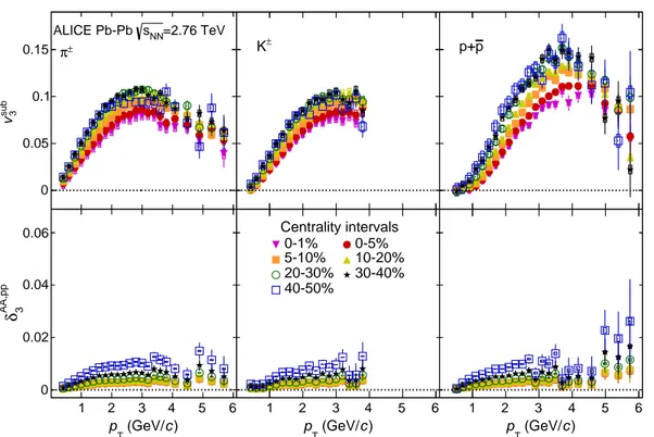
) c (GeV/ T p 1 2 3 4 5 6 sub 3 v 0 0.05 0.1 0.15 _π± =2.76 TeV NN s ALICE Pb-Pb ) c (GeV/ T p 1 2 3 4 5 6 3 AA,pp δ 0 0.02 0.04 0.06 pT (GeV/c) 1 2 3 4 5 6 sub 3 v 0 0.05 0.1 0.15 K± ) c (GeV/ T p 1 2 3 4 5 6 3 AA,pp _δ 0 0.02 0.04 0.06 Centrality intervals 0-1% 0-5% 5-10% 10-20% 20-30% 30-40% 40-50% ) c (GeV/ T p 1 2 3 4 5 6 sub 3 v 0 0.05 0.1 0.15 p+p ) c (GeV/ T p 1 2 3 4 5 6 3 AA,pp _δ 0 0.02 0.04 0.06

Fig. 3: The pT-differential vsub3 (top row) and δ AA,pp

3 (bottom row) for different centralities in Pb–Pb collisions at

√

sNN= 2.76 TeV grouped by particle species.

) c (GeV/ T p 1 2 3 4 5 6 sub 4 v 0 0.05 0.1 0.15 _π± =2.76 TeV NN s ALICE Pb-Pb ) c (GeV/ T p 1 2 3 4 5 6 4 AA,pp δ 0 0.02 0.04 0.06 pT (GeV/c) 1 2 3 4 5 6 sub 4 v 0 0.05 0.1 0.15 K± ) c (GeV/ T p 1 2 3 4 5 6 4 AA,pp _δ 0 0.02 0.04 0.06 Centrality intervals 0-1% 0-5% 5-10% 10-20% 20-30% 30-40% 40-50% ) c (GeV/ T p 1 2 3 4 5 6 sub 4 v 0 0.05 0.1 0.15 p+p ) c (GeV/ T p 1 2 3 4 5 6 4 AA,pp _δ 0 0.02 0.04 0.06

Fig. 4: The pT-differential vsub4 (top row) and δ AA,pp

4 (bottom row) for different centralities in Pb–Pb collisions at

√

) c (GeV/ T p 1 2 3 4 5 6 sub 5 v 0 0.05 0.1 ± π =2.76 TeV NN s ALICE Pb-Pb ) c (GeV/ T p 1 2 3 4 5 6 5 AA,pp δ 0 0.02 0.04 0.06 pT (GeV/c) 1 2 3 4 5 6 sub 5 v 0 0.05 0.1 ± K ) c (GeV/ T p 1 2 3 4 5 6 5 AA,pp _δ 0 0.02 0.04 0.06 Centrality intervals 0-1% 0-5% 5-10% 10-20% 20-30% 30-40% 40-50% ) c (GeV/ T p 1 2 3 4 5 6 sub 5 v 0 0.05 0.1 p p+ ) c (GeV/ T p 1 2 3 4 5 6 5 AA,pp _δ 0 0.02 0.04 0.06

Fig. 5: The pT-differential vsub5 (top row) and δ AA,pp

5 (bottom row) for different centralities in Pb–Pb collisions at

√

sNN= 2.76 TeV grouped by particle species.

particle species and it is due to the interplay between the decrease in multiplicity and the corresponding increase in reference flow as one goes towards more peripheral collisions.

Similar to Fig. 2, Figs. 3, 4 and 5 present the pT-differential vsub₃ , vsub₄ and vsub₅ (top rows), respectively,

and the corresponding subtracted terms (bottom rows) for pions, kaons and protons measured in different centrality intervals. One observes that all vsubn have significant non-zero values throughout the entire

measured pT range for ultra-central collisions, where the main contributors to the initial

coordinate-space anisotropies, which are necessary for the development of vsubn , are supposed to be the fluctuations

of the initial density profile [16]. In addition, the values of the higher flow harmonics increase from ultra-central collisions (0–1%) to the most peripheral collisions (40–50%). However, this increase as a function of centrality is smaller in comparison to vsub₂ . Thus, vsub₂ seems to mainly reflect the initial geometry of the system while the higher-order flow harmonics are affected less. The non-vanishing values of these higher-order flow harmonics are consistent with the notion in which they are generated primarily from the event-by-event fluctuations of the initial energy density profile.

In addition, all flow harmonics show a monotonic increase with increasing pT up to 3 GeV/c reaching a

maximum that depends on the particle species and on the collision centrality. In particular, the position of this maximum of vsubn (pT) exhibits a centrality dependence due to the change in radial flow which

becomes larger for central compared to peripheral collisions. Moreover, this maximum seems to have a particle mass dependence as well, since it takes place at a higher pT value for heavier particles in each

centrality interval.

The lower panel of Figs. 3, 4 and 5 also illustrate the magnitude of δnAA,ppas a function of pT. In these

cases, δ₃AA,pp varies between 5% and 8% relative to vAA₃ , δ₄AA,ppbetween 12% and 18% with respect to vAA₄ , and δ₅AA,ppbetween 12% and 20% with respect to vAA₅ . Similar to δ₂AA,pp, the variation in the value of higher harmonic δnAA,ppis derived from the decrease in multiplicity and the increasing reference flow

in the transition from central to more peripheral collisions.

6.2 Evolution of flow harmonics in ultra-central Pb–Pb collisions

Figure 6 shows the evolution of different flow harmonics for π±(left column), K±(middle column) and p+p (right column) for ultra-central (i.e. 0–1%) collisions in comparison to the other centrality intervals. For ultra-central Pb–Pb collisions one expects the influence of the collision geometry to the development of vsubn to be reduced compared to the contribution of initial energy-density fluctuations. Figure 6 shows

that for pions the value of vsub₃ is equal to vsub₂ at around pT ≈ 1 GeV/c and becomes the dominant

harmonic for higher transverse momenta. Furthermore, vsub₄ at pT≈ 2 GeV/c and vsub₅ at around pT ≈ 3

GeV/c become equal to vsub₂ . For higher transverse momentum values, vsub₄ becomes gradually larger than vsub₂ reaching a similar magnitude as vsub₃ at around 3.5 GeV/c, while vsub₅ remains equal to vsub₂ . As the collisions become more peripheral, one expects that geometry becomes a significant contributor to the development of azimuthal anisotropy. As a result, vsub₂ is the dominant harmonic for peripheral collisions throughout the entire measured momentum range. Furthermore, vsub₃ , vsub₄ and vsub₅ seem to have similar magnitudes and pTevolution as observed in ultra-central Pb–Pb events, indicating a smaller

influence of the collision geometry in their development than for vsub₂ .

For kaons and protons, one observes a similar trend in the pT evolution of vsub2 , vsub3 , vsub4 and vsub5 as

for pions. However, the flow harmonics for ultra-central collisions (top middle and right plots of Fig. 6 respectively) exhibit a crossing that takes place at pT values that change as a function of the particle

mass. For kaons, the crossing between vsub₂ and vsub₃ occurs at higher pT (≈1.4 GeV/c) compared to

pions while for protons it occurs at an even higher pT value (≈1.8 GeV/c). Similarly, the vsub₂ and

vsub₄ crossing occurs higher in pT for kaons (≈2.2 GeV/c) and protons (≈2.8 GeV/c) as compared to

pions. The values of vsub₄ for kaons reach a similar magnitude to vsub₃ at around 3.5 GeV/c and this takes place at around 4 GeV/c for protons. The dependence of the crossing between different flow harmonics, and thus the range where a given harmonic becomes dominant, on the particle mass can be attributed to the interplay of not only elliptic but also triangular and quadrangular flow with radial flow.

6.3 Mass ordering

The interplay between the different flow harmonics and radial flow can be further probed by studying how vsub_n (pT) develops as a function of the particle mass for various centralities. In Ref. [23], it was clearly

demonstrated that the interplay between radial and elliptic flow leads to a characteristic mass ordering at pT < 2–3 GeV/c. This mass ordering originates from the fact that radial flow creates a depletion

in the particle spectrum at low pT values, which increases with increasing particle mass and transverse

velocity. When this effect is embedded in an environment where azimuthal anisotropy develops, it leads to heavier particles having smaller vsubn values compared to lighter ones at given values of pT. It is thus

interesting to study whether the interplay between the anisotropic flow harmonics and radial flow leads also to a mass ordering in vsubn (pT) for n > 2.

Figure 7–left presents the pT-differential vsub2 for charged pions, kaons and protons starting from

ultra-central collisions up to the 40–50% ultra-centrality interval. The observed evolution of vsub₂ with mass confirms that the interplay between elliptic and radial flow leads to lower vsub₂ values at fixed pT for heavier

particles for pT< 2–3 GeV/c, depending on the centrality interval.

Similarly, Figs. 7–right, 8–left and 8–right show the pT-differential vsub₃ , vsub₄ and vsub₅ , respectively, for

different particle species and for each centrality interval. A clear mass ordering is seen in the low pT

re-gion, i.e. for pT < 2–3 GeV/c, for vsub3 (pT), v4sub(pT) and vsub5 (pT), which arises from the interplay

between the anisotropic flow harmonics and radial flow.

1 2 3 4 5 0 0.05 0.1 _π0-1%_± 1 2 3 4 5 0 0.05 0.1 π± 0-5% 1 2 3 4 5 0 0.05 0.1 0.15 _± π 5-10% 1 2 3 4 5 sub n v 0 0.1 0.2 π± 10-20% 1 2 3 4 5 0 0.1 0.2 0.3 ± π 20-30% 1 2 3 4 5 0 0.1 0.2 0.3 ± π 30-40% 1 2 3 4 5 0 0.1 0.2 0.3 ± π 40-50% 1 2 3 4 5 0 0.05 0.1 _KALICE Pb-Pb ± sNN=2.76 TeV sub 2 v sub 3 v sub 4 v sub 5 v 1 2 3 4 5 0 0.05 0.1 K± 1 2 3 4 5 0 0.05 0.1 0.15 _± K 1 2 3 4 5 0 0.1 0.2 K± 1 2 3 4 5 0 0.1 0.2 0.3 ± K 1 2 3 4 5 0 0.1 0.2 0.3 ± K ) c (GeV/ T p 1 2 3 4 5 0 0.1 0.2 0.3 ± K 1 2 3 4 5 0 0.05 0.1 _p+p 1 2 3 4 5 0 0.05 0.1 p+p 1 2 3 4 5 0 0.05 0.1 0.15 p p+ 1 2 3 4 5 0 0.1 0.2 p+p 1 2 3 4 5 0 0.1 0.2 0.3 p p+ 1 2 3 4 5 0 0.1 0.2 0.3 p p+ 1 2 3 4 5 0 0.1 0.2 0.3 p p+

Fig. 6: The evolution of the pT-differential vsubn for π±, K± and p+p, in the left, middle and right columns,

respectively, grouped by centrality interval in Pb–Pb collisions at√sNN= 2.76 TeV.

the centrality and the order of the flow harmonic, takes place at different pT values. In Figs. 7 and 8 it

) c (GeV/ T p 1 2 3 4 5 sub 2 v 0 0.05 0-1% ) c (GeV/ T p 1 2 3 4 5 sub 2 v 0 0.05 0.1 0.15 0-5% ) c (GeV/ T p 1 2 3 4 5 sub 2 v 0 0.1 0.2 10-20% ) c (GeV/ T p 1 2 3 4 5 sub 2 v 0 0.1 0.2 0.3 30-40% =2.76 TeV NN s ALICE Pb-Pb Particle species ± π ± K p p+ ) c (GeV/ T p 1 2 3 4 5 sub 2 v 0 0.05 0.1 0.15 5-10% ) c (GeV/ T p 1 2 3 4 5 sub 2 v 0 0.1 0.2 20-30% ) c (GeV/ T p 1 2 3 4 5 sub 2 v 0 0.1 0.2 0.3 40-50% ) c (GeV/ T p 1 2 3 4 5 sub 3 v 0 0.05 0.1 0-1% ) c (GeV/ T p 1 2 3 4 5 sub 3 v 0 0.05 0.1 0.15 0-5% ) c (GeV/ T p 1 2 3 4 5 sub 3 v 0 0.05 0.1 0.15 10-20% ) c (GeV/ T p 1 2 3 4 5 sub 3 v 0 0.05 0.1 0.15 30-40% =2.76 TeV NN s ALICE Pb-Pb Particle species ± π ± K p p+ ) c (GeV/ T p 1 2 3 4 5 sub 3 v 0 0.05 0.1 0.15 5-10% ) c (GeV/ T p 1 2 3 4 5 sub 3 v 0 0.05 0.1 0.15 20-30% ) c (GeV/ T p 1 2 3 4 5 sub 3 v 0 0.05 0.1 0.15 40-50%

Fig. 7: The pT-differential vsub2 (left figure) and vsub3 (right figure) for different particle species grouped by centrality

class in Pb–Pb collisions at√sNN= 2.76 TeV.

) c (GeV/ T p 1 2 3 4 5 sub 4 v 0 0.05 0.1 0-1% ) c (GeV/ T p 1 2 3 4 5 sub 4 v 0 0.05 0.1 0-5% ) c (GeV/ T p 1 2 3 4 5 sub 4 v 0 0.05 0.1 0.15 10-20% ) c (GeV/ T p 1 2 3 4 5 sub 4 v 0 0.05 0.1 0.15 30-40% =2.76 TeV NN s ALICE Pb-Pb Particle species ± π ± K p p+ ) c (GeV/ T p 1 2 3 4 5 sub 4 v 0 0.05 0.1 5-10% ) c (GeV/ T p 1 2 3 4 5 sub 4 v 0 0.05 0.1 0.15 20-30% ) c (GeV/ T p 1 2 3 4 5 sub 4 v 0 0.05 0.1 0.15 40-50% ) c (GeV/ T p 1 2 3 4 5 sub 5 v 0 0.05 0.1 _0-1% ) c (GeV/ T p 1 2 3 4 5 sub 5 v 0 0.05 0.1 _0-5% ) c (GeV/ T p 1 2 3 4 5 sub 5 v 0 0.05 0.1 _10-20% ) c (GeV/ T p 1 2 3 4 5 sub 5 v 0 0.05 0.1 30-40% =2.76 TeV NN s ALICE Pb-Pb Particle species ± π ± K p p+ ) c (GeV/ T p 1 2 3 4 5 sub 5 v 0 0.05 0.1 _5-10% ) c (GeV/ T p 1 2 3 4 5 sub 5 v 0 0.05 0.1 _20-30% ) c (GeV/ T p 1 2 3 4 5 sub 5 v 0 0.05 0.1 40-50%

Fig. 8: The pT-differential vsub4 (left figure) and vsub5 (right figure) for different particle species grouped by centrality

) c (GeV/ q n / T p 0.5 1 1.5 2 2.5 q n/ sub 2 v 0 0.01 0.02 0.03 0-1% ) c (GeV/ q n / T p 0.5 1 1.5 2 2.5 q n/ sub 2 v 0 0.02 0.04 0.06 _0-5% ) c (GeV/ q n / T p 0.5 1 1.5 2 2.5 q n/ sub 2 v 0 0.05 0.1 10-20% ) c (GeV/ q n / T p 0.5 1 1.5 2 2.5 q n/ sub 2 v 0 0.05 0.1 0.15 30-40% =2.76 TeV NN s ALICE Pb-Pb Particle species ± π ± K p p+ ) c (GeV/ q n / T p 0.5 1 1.5 2 2.5 q n/ sub 2 v 0 0.02 0.04 0.06 _5-10% ) c (GeV/ q n / T p 0.5 1 1.5 2 2.5 q n/ sub 2 v 0 0.05 0.1 20-30% ) c (GeV/ q n / T p 0.5 1 1.5 2 2.5 q n/ sub 2 v 0 0.05 0.1 0.15 40-50% ) c (GeV/ q n / T p 0.5 1 1.5 2 2.5 q n/ sub 3 v 0 0.02 0.04 0.06 0-1% ) c (GeV/ q n / T p 0.5 1 1.5 2 2.5 q n/ sub 3 v 0 0.02 0.04 0.06 0-5% ) c (GeV/ q n / T p 0.5 1 1.5 2 2.5 q n/ sub 3 v 0 0.02 0.04 0.06 10-20% ) c (GeV/ q n / T p 0.5 1 1.5 2 2.5 q n/ sub 3 v 0 0.02 0.04 0.06 _30-40% =2.76 TeV NN s ALICE Pb-Pb Particle species ± π ± K p p+ ) c (GeV/ q n / T p 0.5 1 1.5 2 2.5 q n/ sub 3 v 0 0.02 0.04 0.06 5-10% ) c (GeV/ q n / T p 0.5 1 1.5 2 2.5 q n/ sub 3 v 0 0.02 0.04 0.06 20-30% ) c (GeV/ q n / T p 0.5 1 1.5 2 2.5 q n/ sub 3 v 0 0.02 0.04 0.06 _40-50%

Fig. 9: The pT/nqdependence of vsub2 /nq(left figure) and vsub3 /nq(right figure) for π±, K±and p+p for Pb–Pb

collisions in various centrality intervals at√sNN= 2.76 TeV.

comparison to more central events. The crossing point for central collisions occurs at higher pT values

for vsubn since the common velocity field, which exhibits a significant centrality dependence, affects heavy

particles more. The current study shows that this occurs not only in the case of elliptic flow but also for higher flow harmonics. Finally, beyond the crossing point for each centrality and for every harmonic, it is seen that particles tend to group based on their number of constituent quarks. This apparent grouping will be discussed in the next subsection.

6.4 Test of scaling properties

It was first observed at RHIC that at intermediate values of transverse momentum (3 < pT< 6 GeV/c)

the value of v2 for baryons is larger than that of mesons [19–22]. As a result it was suggested that if

both vn and pT are scaled by the number of constituent quarks (nq), the resulting pT/nq dependence of

the scaled values for all particle species will have an approximate similar magnitude and dependence on scaled transverse momentum. This scaling, known as number of constituent quark scaling (NCQ), worked fairly well at RHIC energies, although later measurements revealed sizeable deviations from a perfect scaling [30]. Recently, ALICE measurements [23] showed that the NCQ scaling at LHC energies holds at an approximate level of ±20% for vAA₂ .

Although the scaling is only approximate, it stimulated various theoretical ideas that attempted to address its origin. As a result, several models [28, 29] attempted to explain this observed effect by requiring quark coalescence to be the dominant particle production mechanism in the intermediate pTregion, where the

hydrodynamic evolution of the fireball is not the driving force behind the development of anisotropic flow.

Figures 9 and 10 present vsub₂ and vsub₃ , as well as vsub₄ and vsub₅ , respectively, scaled by the number of constituent quarks (nq) as a function of pT/nqfor π±, K±and p+p grouped in centrality bins. Figure 9–

) c (GeV/ q n / T p 0.5 1 1.5 2 2.5 q n/ sub 4 v 0 0.02 0.04 0.06 0-1% ) c (GeV/ q n / T p 0.5 1 1.5 2 2.5 q n/ sub 4 v 0 0.02 0.04 0.06 0-5% ) c (GeV/ q n / T p 0.5 1 1.5 2 2.5 q n/ sub 4 v 0 0.02 0.04 0.06 10-20% ) c (GeV/ q n / T p 0.5 1 1.5 2 2.5 q n/ sub 4 v 0 0.02 0.04 0.06 30-40% =2.76 TeV NN s ALICE Pb-Pb Particle species ± π ± K p p+ ) c (GeV/ q n / T p 0.5 1 1.5 2 2.5 q n/ sub 4 v 0 0.02 0.04 0.06 5-10% ) c (GeV/ q n / T p 0.5 1 1.5 2 2.5 q n/ sub 4 v 0 0.02 0.04 0.06 20-30% ) c (GeV/ q n / T p 0.5 1 1.5 2 2.5 q n/ sub 4 v 0 0.02 0.04 0.06 40-50% ) c (GeV/ q n / T p 0.5 1 1.5 2 2.5 q n/ sub 5 v 0 0.02 0.04 0-1% ) c (GeV/ q n / T p 0.5 1 1.5 2 2.5 q n/ sub 5 v 0 0.02 0.04 0-5% ) c (GeV/ q n / T p 0.5 1 1.5 2 2.5 q n/ sub 5 v 0 0.02 0.04 10-20% ) c (GeV/ q n / T p 0.5 1 1.5 2 2.5 q n/ sub 5 v 0 0.02 0.04 30-40% =2.76 TeV NN s ALICE Pb-Pb Particle species ± π ± K p p+ ) c (GeV/ q n / T p 0.5 1 1.5 2 2.5 q n/ sub 5 v 0 0.02 0.04 5-10% ) c (GeV/ q n / T p 0.5 1 1.5 2 2.5 q n/ sub 5 v 0 0.02 0.04 20-30% ) c (GeV/ q n / T p 0.5 1 1.5 2 2.5 q n/ sub 5 v 0 0.02 0.04 40-50%

Fig. 10: The pT/nqdependence of vsub4 /nq(left figure) and vsub5 /nq(right figure) for π±, K±and p+p for Pb–Pb

collisions in various centrality intervals at√sNN= 2.76 TeV.

this scaling holds at the same level (±20%) within the current statistical and systematic uncertainties. 6.5 Comparison with models

Measurements of vAAn at RHIC and LHC have been successfully described by hydrodynamical

calcula-tions. In particular in [23] it was shown that a hybrid model that couples the hydrodynamical expansion of the fireball to a hadronic cascade model describing the final-state hadronic interactions is able to re-produce the basic features of the measurements at low values of pT. In parallel, various other models that

incorporate a different description of the dynamical evolution of the system, such as AMPT, are also able to describe some of the main features of measurements of azimuthal anisotropy [50–52]. In this section, these two different theoretical approaches will be confronted with the experimental measurements. 6.5.1 Comparison with iEBE-VISHNU

Figures 11, 12 and 13 present the comparison between the ALICE measurements of vsubn and recent

vnhydrodynamical calculations from [49]. These calculations are based on iEBE-VISHNU, an

event-by-event version of the VISHNU hybrid model [54] which couples 2+1 dimensional viscous hydrodynamics (VISH2+1) to a hadron cascade model (UrQMD) [55] and uses a set of fluctuating initial conditions generated with AMPT. The iEBE-VISHNU model makes it possible to study the influence of the hadronic stage on the development of elliptic flow and higher harmonics for different particles. In this model, the initial time after which the hydrodynamic evolution begins is set to τ0 = 0.4 fm/c and the transition

between the macroscopic and microscopic approaches takes place at a temperature of T = 165 MeV. Finally, the value of the shear viscosity to entropy density ratio is chosen to be η/s = 0.08, corresponding to the conjectured lower limit discussed in the introduction. These input parameters were chosen to best fit the multiplicity and transverse momentum spectra of charged particles in most central Pb–Pb collisions as well as the pT-differential v2, v3, and v4for charged particles for various centrality intervals.

) c (GeV/ T p 0.5 1 1.5 2 2.5 2 v 0 0.1 0.2 0.3 ALICE 10-20% ± π_± K p p+ iEBE-VISHNU ± π_± K p p+ ) c (GeV/ T p 0.5 1 1.5 2 2.5 2 v ∆ 0.01 − 0 0.01 ) c (GeV/ T p 0.5 1 1.5 2 2.5 2 v 0 0.1 0.2 0.3 Pb-Pb sNN=2.76 TeV 20-30% ) c (GeV/ T p 0.5 1 1.5 2 2.5 2 v ∆ 0.01 − 0 0.01 ) c (GeV/ T p 0.5 1 1.5 2 2.5 2 v 0 0.1 0.2 0.3 30-40% ) c (GeV/ T p 0.5 1 1.5 2 2.5 2 v ∆ 0.01 − 0 0.01 ) c (GeV/ T p 0.5 1 1.5 2 2.5 2 v 0 0.1 0.2 0.3 40-50% ) c (GeV/ T p 0.5 1 1.5 2 2.5 2 v ∆ 0.01 − 0 0.01

Fig. 11: The pT-differential vsub₂ for pions, kaons and protons measured with the Scalar Product method in Pb–

Pb collisions at√sNN= 2.76 TeV compared to v2measured with iEBE-VISHNU. The upper panels present the

comparison for 10–20% up to 40–50% centrality intervals. The thickness of the curves reflect the uncertainties

of the hydrodynamical calculations. The differences between vsub

2 from data and v2 from iEBE-VISHNU are

presented in the lower panels.

These figures show that this hydrodynamical calculation can reproduce the observed mass ordering in the experimental data for pions, kaons and protons. In particular, it is seen that for the range 1 < pT< 2

GeV/c in the 10–20% centrality interval the model overpredicts the pion vsub₂ (pT) values by an average

of 10%, however for more peripheral collisions the curve describes the data points relatively well. In addition, the model describes vsub₃ and vsub₄ for charged pions within 5%, i.e. better than vsub₂ . Further-more, it is seen that iEBE-VISHNU overpredicts the vsub₂ (pT) values of K± (i.e. 10–15% deviations)

and does not describe p+p in more central collisions (i.e. by 10% with a different transverse momentum dependence compared to data), but in more peripheral collisions the agreement with the data points is better. Finally, the model describes the vsub₃ (pT) and vsub₄ (pT) values for K± and p+p with a reasonable

accuracy (i.e. within 5%) in all centrality intervals up to pTaround 2 GeV/c. These observations are also

illustrated in the lower plots of each panel in Figs. 11, 12 and 13 that present the difference between the measured vsubn relative to a fit to the hydrodynamical calculation.

6.5.2 Comparison with AMPT

In addition to the hydrodynamical calculations discussed in the previous paragraphs, three different ver-sions of AMPT [50–52] are studied in this article. The AMPT model can be run in two main configura-tions: the default and the string melting. In the default version, partons are recombined with the parent strings when they stop interacting. The resulting strings are later converted into hadrons using the Lund string fragmentation model [56, 57]. In the string melting version, the initial strings are melted into par-tons whose interactions are described by a parton cascade model [58]. These parpar-tons are then combined

) c (GeV/ T p 0.5 1 1.5 2 2.5 3 v 0 0.05 0.1 0.15 10-20% ALICE ± π_± K p p+ iEBE-VISHNU ± π_± K p p+ ) c (GeV/ T p 0.5 1 1.5 2 2.5 3 v ∆ 0.01 − 0 0.01 ) c (GeV/ T p 0.5 1 1.5 2 2.5 3 v 0 0.05 0.1 0.15 =2.76 TeV NN s Pb-Pb 20-30% ) c (GeV/ T p 0.5 1 1.5 2 2.5 3 v ∆ 0.01 − 0 0.01 ) c (GeV/ T p 0.5 1 1.5 2 2.5 3 v 0 0.05 0.1 0.15 30-40% ) c (GeV/ T p 0.5 1 1.5 2 2.5 3 v ∆ 0.01 − 0 0.01 ) c (GeV/ T p 0.5 1 1.5 2 2.5 3 v 0 0.05 0.1 0.15 40-50% ) c (GeV/ T p 0.5 1 1.5 2 2.5 3 v ∆ 0.01 − 0 0.01

Fig. 12: The pT-differential vsub₃ for pions, kaons and protons measured with the Scalar Product method in Pb–

Pb collisions at√sNN= 2.76 TeV compared to v3measured with iEBE-VISHNU. The upper panels present the

comparison for 10–20% up to 40–50% centrality intervals. The thickness of the curves reflect the uncertainties

of the hydrodynamical calculations. The differences between vsub

3 from data and v3 from iEBE-VISHNU are

presented in the lower panels.

into the final-state hadrons via a quark coalescence model. In both configurations a final-state hadronic rescattering is implemented which also includes resonance decays. The third version presented in this article is based on the string melting configuration, in which the hadronic rescattering phase is switched off to study its influence to the development of anisotropic flow. The input parameters used in all cases are: αs= 0.33, a partonic cross-section of 1.5 mb, while the Lund string fragmentation parameters were

set to α = 0.5 and b = 0.9 GeV−2.

Figure 14 presents the pT-differential v2(first row), v3(middle row) and v4(bottom row) for pions, kaons

and protons for the 20–30% centrality interval. Each column presents the results of one of the three AMPT versions discussed above. The string melting AMPT version (left column) predicts a distinct mass ordering at low values of transverse momentum as well as a lower value of vnfor mesons compared

to baryons in the intermediate pTregion for all harmonics, similar to what is observed in the experimental

measurements. On the other hand, the version with string melting but without the hadronic rescattering contribution (middle column) can only reproduce the particle type grouping at intermediate pT values.

Finally, the default AMPT version is only able to reproduce the mass ordering in the low pTregion. These

observations suggest that the string melting and the final-state hadronic rescattering are responsible for the particle type grouping at intermediate pTand the mass ordering at low pT, respectively.

Since the AMPT string melting version is able to reproduce the main features of the experimental mea-surement throughout the reported pTrange, the corresponding results are compared with the data points

in Fig. 15. It is seen that although this version of AMPT reproduces both the mass ordering and the par-ticle type grouping at low and intermediate pT for all harmonics, it fails to quantitatively reproduce the

) c (GeV/ T p 0.5 1 1.5 2 2.5 4 v 0 0.05 0.1 0.15 10-20% ALICE ± π_± K p p+ iEBE-VISHNU ± π_± K p p+ ) c (GeV/ T p 0.5 1 1.5 2 2.5 4 v ∆ 0.01 − 0 0.01 ) c (GeV/ T p 0.5 1 1.5 2 2.5 4 v 0 0.05 0.1 0.15 =2.76 TeV NN s Pb-Pb 20-30% ) c (GeV/ T p 0.5 1 1.5 2 2.5 4 v ∆ 0.01 − 0 0.01 ) c (GeV/ T p 0.5 1 1.5 2 2.5 4 v 0 0.05 0.1 0.15 30-40% ) c (GeV/ T p 0.5 1 1.5 2 2.5 4 v ∆ 0.01 − 0 0.01 ) c (GeV/ T p 0.5 1 1.5 2 2.5 4 v 0 0.05 0.1 0.15 40-50% ) c (GeV/ T p 0.5 1 1.5 2 2.5 4 v ∆ 0.01 − 0 0.01

Fig. 13: The pT-differential vsub₄ for pions, kaons and protons measured with the Scalar Product method in Pb–

Pb collisions at√sNN= 2.76 TeV compared to v4measured with iEBE-VISHNU. The upper panels present the

comparison for 10–20% up to 40–50% centrality intervals. The thickness of the curves reflect the uncertainties

of the hydrodynamical calculations. The differences between vsub

4 from data and v4 from iEBE-VISHNU are

presented in the lower panels.

measurements. In order to understand the origin of this discrepancy both spectra and the pT-differential

vsub₂ for different particle species for the 20–30% centrality interval in AMPT were fitted with a blast-wave parametrisation [59]. The results were compared to the analogous parameters obtained from the experiment [43]. It turns out that the radial flow in AMPT is around 25% lower than the measured value at the LHC. As the radial flow is essential in shaping the pT dependence of vsubn we suppose that the

unrealistically low radial flow in AMPT is responsible for the quantitative disagreement.

7 Conclusions

In this article, a measurement of non-flow subtracted flow harmonics, vsub₂ , vsub₃ , vsub₄ and vsub₅ as a function of transverse momentum for π±, K± and p+p for different centrality intervals (0–1% up to 40–50%) in Pb–Pb collisions at √s_NN = 2.76 TeV are reported. The vsubn coefficients are calculated with the

Scalar Product method, selecting the identified hadron under study and the reference flow particles from different, non-overlapping pseudorapidity regions. Correlations not related to the common symmetry planes (i.e. non-flow) were estimated based on pp collisions and were subtracted from the measurements. The validity of this subtraction procedure was checked by repeating the analysis using different charge combinations (i.e. positive–positive and negative–negative) for the identified hadrons and the reference particles collisions as well as applying different pseudorapidity gaps (∆η) between them, in both Pb–Pb and pp collisions. The results after the subtraction in both cases did not exhibit any systematic change in

) c (GeV/ T p 0.5 1 1.5 2 2.5 2 v 0.1 0.2 0.3 string melting ) c (GeV/ T p 0.5 1 1.5 2 2.5 3 v 0.05 0.1 0.15 ) c (GeV/ T p 0.5 1 1.5 2 2.5 4 v 0 0.05 0.1 ) c (GeV/ T p 0.5 1 1.5 2 2.5 2 v 0.1 0.2

0.3 string melting without_{hadronic rescattering}

) c (GeV/ T p 0.5 1 1.5 2 2.5 3 v 0.05 0.1 0.15 AMPT ± π ± K p p+ ) c (GeV/ T p 0.5 1 1.5 2 2.5 4 v 0 0.05 0.1 ) c (GeV/ T p 0.5 1 1.5 2 2.5 2 v 0.1 0.2 0.3 default ) c (GeV/ T p 0.5 1 1.5 2 2.5 3 v 0.05 0.1 0.15 ) c (GeV/ T p 0.5 1 1.5 2 2.5 4 v 0 0.05 0.1 Fig. 14: The vAA

2 (pT), vAA3 (pT) and vAA4 (pT) in 20–30% central Pb–Pb collisions at √

sNN= 2.76 TeV, obtained

using the string melting, with (left) and without (middle) hadronic rescattering, and the default (right) versions.

vsub_n (pT) with respect to the default ones for any particle species or centrality.

All flow harmonics exhibit an increase in peripheral compared to central collisions. This increase is more pronounced for vsub₂ than for the higher harmonics. This indicates that vsub₂ reflects mainly the geometry of the system, while higher order flow harmonics are primarily generated by event-by-event fluctuations of the initial energy density profile. This is also supported by the observation of a significant non-zero value of vsubn > 0 in ultra-central (i.e. 0–1%) collisions. In this centrality interval of Pb–Pb collisions, vsub3 and

vsub₄ become gradually larger than vsub₂ at a transverse momentum value which increases with increasing order of the flow harmonics and particle mass. In addition, a distinct mass ordering is observed for all vsubn coefficients in all centrality intervals in the low transverse momentum region, i.e. for pT < 3

GeV/c. Furthermore, the vsubn (pT) values show a crossing between π±, K± and p+p, that takes place at

different pT values depending on the centrality and the order of the flow harmonic. These observations

are attributed to the interplay between not only vsub₂ but also the higher flow harmonics and radial flow. For transverse momentum values beyond the crossing point between different particle species (i.e. for pT > 3 GeV/c), the values of vsubn for baryons are larger than for mesons. The NCQ scaling holds for

vsub₂ at an approximate level of ±20% which is in agreement with [23]. For higher harmonics this scaling holds at a similar level within the current level of statistical and systematic uncertainties.

In the low momentum region, hydrodynamic calculations based on iEBE-VISHNU describe vsub₂ for all three particle species and vsub₃ and vsub₄ of pions fairly well. For kaons and protons the model seems to