Cellular Automata Methods
in Mathematical Physics
by
Mark Andrew Smith
B.S. (Physics with Astrophysics Option and Mathematics) and
B.S. (Computer Science with Scientific Programming Applications
Option), New Mexico Institute of Mining and Technology,
Socorro, New Mexico (1982)
Submitted to the Department of Physics
in partial fulfillment of the requirements for the degree of
Doctor of Philosophy
at the
MASSACHUSETTS INSTITUTE OF TECHNOLOGY
May 1994
( 1994 Mark A. Smith. All rights reserved.
The author hereby grants to MIT permission to reproduce and
distribute publicly paper and electronic copies of this thesis document
in whole or in part, and to grant others the right to do so.
Author
...
;..-
...
Department of Physics
May 16th, 1994
Certified by..
...- ...
...
Tommaso Toffoli
Principal Research Scientist
Thesis Supervisor
Accepted by ...
George F. Koster, Professor of Physics
Ch
ajrma mental
Graduate
Committee
Cellular Automata Methods
in Mathematical Physics
by
Mark Andrew Smith
Submitted to the Department of Physics
on May 16th, 1994, in partial fulfillment of the requirements for the degree of
Doctor of Philosophy
Abstract
Cellular automata (CA) are fully discrete, spatially-distributed dynamical systems which can serve as an alternative framework for mathematical descriptions of physical systems. Furthermore, they constitute intrinsically parallel models of computation which can be efficiently realized with special-purpose cellular automata machines. The basic objective of this thesis is to determine techniques for using CA to model physical phenomena and to develop the associated mathematics. Results may take the form of simulations and calculations as well as proofs, and applications are suggested
throughout.
We begin by describing the structure, origins, and modeling categories of CA. A general method for incorporating dissipation in a reversible CA rule is suggested by a model of a lattice gas in the presence of an external potential well. Statistical forces are generated by coupling the gas to a low temperature heat bath. The equilibrium state of the coupled system is analyzed using the principle of maximum entropy. Con-tinuous symmetries are important in field theory, whereas CA describe discrete fields. However, a novel CA rule for relativistic diffusion based on a random walk shows how Lorentz invariance can arise in a lattice model. Simple CA models based on the dynamics of abstract atoms are often capable of capturing the universal behaviors of complex systems. Consequently, parallel lattice Monte Carlo simulations of abstract polymers were devised to respect the steric constraints on polymer dynamics. The resulting double space algorithm is very efficient and correctly captures the static and dynamic scaling behavior characteristic of all polymers. Random numbers are impor-tant in stochastic computer simulations; for example, those that use the Metropolis algorithm. A technique for tuning random bits is presented to enable efficient uti-lization of randomness, especially in CA machines. Interesting areas for future CA research include network simulation, long-range forces, and the dynamics of solids. Basic elements of a calculus for CA are proposed including a discrete representation of one-forms and an analog of integration. Eventually, it may be the case that
physi-cists will be able to formulate cellular automata rules in a manner analogous to how they now derive differential equations.
Thesis Supervisor: Tommaso Toffoli Title: Principal Research Scientist
Acknowledgements
The most remarkable thing about MIT is the people one meets here, and it is with great pleasure that I now have the opportunity to thank those who have helped me, directly or indirectly, to complete my graduate studies with a Ph.D. First, I would like to thank my thesis advisor, Tommaso Toffoli, for taking me as a student and for giving me financial support and the freedom to work on whatever I wanted. I would also like to thank my thesis committee members Professors Edmund Bertschinger and Felix Villars for the time they spent in meetings and reading my handouts. Professor Villars showed a keen interest in understanding my work by asking questions, suggesting references, arranging contacts with other faculty members, and providing detailed feedback on my writing. I deeply appreciate the personal interest he took in me and my scientific development. Professor George Koster, who must have the hardest job in the physics department, helped me with numerous administrative matters.
The Information Mechanics Group in the Laboratory for Computer Science has been a refuge for me, and its members have been a primary source of strength. Special thanks is due to Norman Margolus who has always been eager to help whenever I had a problem. He and Carol Collura have made me feel at home here by treating me like family. Norm also blazed the thesis trail for me and my fellow graduate students in the group: Joe Hrgoveic, Mike Biafore, Milan Shah, David Harnanan, and Raissa D'Souza. Being here gave me the opportunity to interact with parade of visiting scientists: Charles Bennett, Gerard Vichniac, Bastien Chopard, Jeff Yepez, PierLuigi Pierini, Bob Fisch, Attilia Zumpano, Fred Commoner, Vincenzo D'Andrea, Leonid Khalfin, Asher Perez, Andreas Califano, Luca de Alfaro, and Pablo Tamayo. I also had the chance to get to know several bright undergraduate students who worked for the group including Rebecca Frankel, Ruben Agin, Jason Quick, Sasha Wood, Conan Dailey, Jan Maessen, and Debbie Fuchs. Finally, I was able to learn from an eclectic group of engineering staff: Tom Cloney, David Zaig, Tom Durgavich, Ken Streeter, Doug Faust, and Harris Gilliam. My gratitude goes out to the entire group for making my time here interesting and enjoyable as well as educational.
I would like to express my appreciation to several members of the support staff: Peggy Berkovitz, Barbara Lobbregt, and Kim Wainwright in physics; Be Hubbard, Joanne Talbot, Anna Pham, David Jones, William Ang, Nick Papadakis, and Scott Blomquist in LCS. Besides generally improving the quality of life, they are the ones who are really responsible for running things and have helped me in countless ways. I am indebted to Professor Yaneer Bar-Yam of Boston University for giving me some exposure to the greater physics community. He was the driving force behind the work on polymers (chapter 5) which led to several papers and conference presenta-tions. The collaboration also gave me the opportunity to work with Yitzhak Rabin, a polymer theorist from Israel, as well as with Boris Ostrovsky and others in the polymer center at Boston University. Yaneer has also shown me uncommon strength and kindness which I can only hope to pick up.
My first years at MIT were ones of great academic isolation, and I would have dropped out long ago if it were not for the fellowship of friends that I got to know at the Thursday night coffee hour in Ashdown House-it was an hour that would often
go on for many. The original gang from my first term included Eugene Gath, John Baez, Monty McGovern, Bob Holt, Brian Oki, Robin Vaughan, Glen Kissel, Richard Sproat, and Dan Heinzen. Later years included David Stanley, Arnout Eikeboom, Rich Koch, Vipul Bhushan, Erik Meyer, and most recently, Nate Osgood and Lily Lee from outside Ashdown. I thank you for the intellectual sustenance and fond memories you have given me. Coffee hour was initiated by housemasters Bob and Carol Hulsizer, and I have probably logged 2000 hours in the dining room that now bears their name. Many thanks to them and the new housemasters, Beth and Vernon Ingram, for holding this and other social activities which have made Ashdown House such an enjoyable place to live.
Finally, I owe my deepest gratitude to my family for their continual love, support, and encouragement. I dedicate this thesis to them.
Support was provided in part by the National Science Foundation, grant no. 8618002-IRI, in part by DARPA, grant no. N00014-89-J-1988, and in part by ARPA, grant no. N00014-93-1-0660.
Contents
1 Cellular Automata Methods in Mathematical Physics 2 Cellular Automata as Models of Nature
2.1 The Structure of Cellular Automata .
2.2 A Brief History of Cellular Automata 2.3 A Taxonomy of Cellular Automata .
2.3.1 Chaotic Rules . . . . 2.3.2 Voting Rules. 2.3.3 Reversible Rules ... 2.3.4 Lattice Gases. 2.3.5 Material Transport. 2.3.6 Excitable Media . 2.3.7 Conventional Computation . . .
3 Reversibility, Dissipation, and Statistical Forces
3.1 Introduction.
3.1.1 Reversibility and the Second Law of Thermodynamics. 3.1.2 Potential Energy and Statistical Forces ...
3.1.3 Overview.
3.2 A CA Model of Potentials and Forces ... 3.2.1 Description of the Model ... 3.2.2 Basic Statistical Analysis ... 3.2.3 A Numerical Example ... 15 19
... .. 19
... ..
24
... ..
26
... ..
27
... ..
29
... ..
33
... ..
35
... ..
38
... ..
40
... ..
43
47... .
47
... .
47
... .
48
... .
50
... .
51
... .
51
... .
56
... .
60
. . . . . . . . . . . . . . . . . . . . . . . . . . . . . . . . . . . . . . . . . . . . . . . . . . . . . . . . . . . . . . . .. . . . .: :3.3 CAM-6 Implementation of the Model
3.3.1 CAM-6 Architecture . . .
3.3.2 Description of the Rule . . 3.3.3 Generalization of the Rule 3.4 The Maximum Entropy State . .
3.4.1 Broken Ergodicity . 3.4.2 Finite Size Effects ... 3.4.3 Revised Statistical Analysis 3.5 Results of Simulation ...
3.6 Applications and Extensions . . . 3.6.1 Microelectronic Devices 3.6.2 Self-organization ... 3.6.3 Heat Baths and Random Ni 3.6.4 Discussion ... 3.7 Conclusions ... . . . . . . . . . . . . . . . . . . . . j... . . . . . . . . . . . . . . . . imbers . . . . . . . .
4 Lorentz Invariance in Cellular Automata
4.1 Introduction.
4.1.1 Relativity and Physical Law . . . 4.1.2 Overview.
4.2 A Model of Relativistic Diffusion .... 4.3 Theory and Experiment ...
4.3.1 Analytic Solution. 4.3.2 CAM Simulation ... 4.4 Extensions and Discussion ...
4.5 Conclusions...
5 Modeling Polymers with Cellular Automata
5.1 Introduction.
5.1.1 Atoms, the Behavior of Matter, and Cellular Automata . . . 5.1.2 Monte Carlo Methods, Polymer Physics, and Scaling ....
. . . 62
... ..65
... ..69
... . .71
... ..72
... . .. 75 ... . .. 76... . .79
... . .81
... . .81
... . .82
... ..85
... . .86
... ..88
91 . . . .91 . . . .91 ... ...92 . . . 94... . .98
... ...98 . . . 99 ... ...103 . . . .106 109 109 109 111 615.1.3 Overview.
5.2 CA Models of Abstract Polymers ... 5.2.1 General Algorithms .
5.2.2 The Double Space Algorithm ... 5.2.3 Comparison with the Bond Fluctuation 5.3 Results of Test Simulations ...
5.4 Applications. ...
5.4.1 Polymer Melts, Solutions, and Gels . . 5.4.2 Pulsed Field Gel Electrophoresis .... 5.5 Conclusions ...
6 Future Prospects for Physical Modeling with
6.1 Introduction.
6.2 Network Modeling.
6.3 The Problem of Forces and Gravitation ....
6.4 The Dynamics of Solids ...
6.4.1 Statement of the Problem ...
6.4.2 Discussion ...
6.4.3 Implications and Applications ...
Cellular Automata
7 Conclusions
A A Microcanocial Heat Bath
A.1 Probabilities and Statistics ...
A.1.1 Derivation of Probabilities ... A.1.2 Alternate Derivation.
A.2 Measuring and Setting the Temperature ... A.3 Additional Thermodynamics .
B Broken Ergodicity and Finite Size Effects
B.1 Fluctuations and Initial Conserved Currents ... B.2 Corrections to the Entropy ...
112 113 115 118 122 124 Method 130 131 134 138 141 141 141 145 148 149 150 152 155 157 157 158 160 162 164 167 167 169
B.3 Statistics of the Coupled System ...
C Canonical Stochastic Weights
C.1 Overview .
C.2 Functions of Boolean Random Variables C.2.1 The Case of Arbitrary Weights C.2.2 The Canonical Weights . C.2.3 Proof of Uniqueness ... C.3 Application in CAM-8 ... C.4 Discussion and Extensions ...
D Differential Analysis of a Relativistic Diffusion Law
D.1 Elementary Differential Geometry, Notation, and Conventions ...
D.1.1 Scalar, Vector, and Tensor Fields ... D.1.2 Metric Geometry.
D.1.3 Minkowski Space ... D.2 Conformal Invariance ...
D.2.1 Conformal Transformations.
D.2.2 The Conformal Group ... D.3 Analytic Solution.
E Basic Polymer Scaling Laws
E.1 Radius of Gyration ... E.2 Rouse Relaxation Time ...
F Differential Forms for Cellular Automata
F.1 Cellular Automata Representations of Physical Fields ... F.2 Scalars and One-Forms ...
F.3 Integration . ... F.3.1 Area ... F.3.2 Winding Number ... 172 175 175 176 177 178 182 183 184 191 192 192 198 200 203 203 206 209 215 216 219 221 221 222 224 225 225 . . . . . . . . . . . . . . . . . . . . . . . . . . . . . . . . . . . . . . . . . . . . . . . . . . . .
F.3.3 Perimeter ... 228
Chapter 1
Cellular Automata Methods in
Mathematical Physics
The objective of this thesis is to explore and develop the potential of cellular au-tomata as mathematical tools for physical modeling. Cellular auau-tomata (CA) have a number of features that make them attractive for simulating and studying physical processes. In addition to having computational advantages, they also offer a precise framework for mathematical analysis. The development proceeds by constructing and then analyzing CA models that resemble a particular physical situation or that illus-trate some physical principle. This in turn leads to a variety of subjects of interest for mathematical physics. The paragraphs below serve as a preview of the major points of this work.
The term cellular automata refers to an intrinsically parallel model of computation that consists of a regular latticework of identical processors that compute in lockstep while exchanging information with nearby processors. Chapter 2 discusses CA in more detail, gives some examples, and reviews some of the ways they have been used. Cellular automata started as mathematical constructs which were not necessarily intended to run on actual computers. However, CA can be efficiently implemented as computer hardware in the form of cellular automata machines, and these machines have sparked a renewed interest in CA as modeling tools. Unfortunately, much of the resulting development in this direction has been limited to "demos" of potential
application areas, and many of the resulting models have been left wanting supporting analysis. This thesis is an effort to improve the situation by putting the field on a more methodical, mathematical tack.
A problem that comes up in many contexts when designing CA rules for physical modeling is the question of how to introduce forces among the constituent parts of a system under consideration. This problem is exacerbated if one wants to obtain an added measure of faithfulness to real physical laws by making the dynamics re-versible. The model presented in chapter 3 gives a technique for generating statistical forces which are derived from an external potential energy function. In the process, it clarifies the how and why of dissipation in the face of microscopic reversibility. The chapter also serves as a paradigm for modeling in statistical mechanics and ther-modynamics using cellular automata machines and shows how one has control over all aspects of a problem-from conception and implementation, through theory and experiment, to application and generalization. Finally, the compact representation of the potential energy function that is used gives one way to represent a physical field and brings up the general problem of representing arbitrary fields.
Many field theories are characterized by symmetries under one or more Lie groups, and it is a problem to reconcile the continuum with the discrete nature of CA. At the finest level, a CA cannot reflect the continuous symmetries of a conventional physical law because of the digital degrees of freedom and the inhomogeneous, anisotropic nature of a lattice. Therefore, the desired symmetry must either arise as a suitable limit of a simple process or emerge as a collective behavior of an underlying complex dynamics. The maximum speed of propagation of information in CA suggests a con-nection with relativity, and chapter 4 shows how a CA model of diffusion can display Lorentz invariance despite having a preferred frame of reference. Kinetic theory can be used to derive the properties of lattice gases, and a basic Boltzmann transport argument leads to a manifestly covariant differential equation for the limiting contin-uum case. The exact solution of this differential equation compares favorably with a CA simulation, and other interesting mathematical properties can be derived as well. One of the most important areas of application of high-performance computation
is that of molecular dynamics, and polymers are arguably the most important kinds of molecules. However, it has proven difficult to devise a Monte Carlo updating scheme that can be run on a parallel computer, while at the same time, CA are inherently parallel. Hence, it is desirable to find CA algorithms for simulating polymers, and this is the starting point for chapter 5. The resulting parallel lattice Monte Carlo polymer dynamics should be of widespread interest in fields ranging from biology and chemical engineering to condensed matter theory. In addition to the theory of scaling, there are a number of mathematical topics which are related to this area such as the study of the geometry and topology of structures in complex fluids. Another is the generation and utilization of random numbers which is important, for example, in the control of chemical reaction rates. Many modifications to the basic method are possible and a model of pulsed field gel electrophoresis is given as an application.
The results obtained herein still represent the early stages of development of CA as general-purpose mathematical modeling tools, and chapter 6 discusses the future prospects along with some outstanding problems. Cellular automata may be applied to any system that has an extended space and that can be given a dynamics, and this includes a very broad class of problems indeed! Each problem requires significant creativity, and the search for solutions will inevitably generate new mathematical concepts and techniques of interest to physicists. Additional topics suggested here are the simulation of computer networks as well as the problems of long-range forces and the dynamics of solids. Besides research on specific basic and applied problems, many mathematical questions remain along with supporting work to be done on hardware and software.
The bulk of this document is devoted to describing a variety of results related to modeling with CA, while chapter 7 summarizes the main contributions and draws some conclusions as sketched below. The appendices are effectively supplementary chapters containing details which are somewhat outside the main line of development, although they should be considered an integral part of the work. They primarily consist of calculations and proofs, but the accompanying discussions are important as well.
Inventing CA models serves to answer the question of what CA are naturally ca-pable of doing and how, but it is during the process of development that the best-the unanticipated-discoveries are made. The simplicity of CA means that one is forced to capture essential phenomenology in abstract form, and this makes for an interest-ing way to find out what features of a system are really important. In the course of presenting a number of modeling techniques, this thesis exemplifies a methodology for generating new topics in mathematical physics. And in addition to giving results on previously unsolved problems, it identifies related research problems which range in difficulty from straightforward to hard to impossible. This in turn encourages con-tinued progress in the field. In conclusion, CA have a great deal of unused potential as mathematical modeling tools for physics; furthermore, they will see more and more applications in the study of complex dynamical systems across many disciplines.
Chapter 2
Cellular Automata as Models of
Nature
This chapter introduces cellular automata (CA) and reviews some of the ways they have been used to model nature. The first section describes the basic format of CA, along with some possible variations. Next, the origins and history of CA are briefly summarized, continuing through to current trends. The last section gives a series of prior applications which illustrate a wide range of phenomena, techniques, concepts, and principles. The examples are organized into categories, and special features are pointed out for each model.
2.1 The Structure of Cellular Automata
Cellular automata can be described in several ways. The description which is perhaps most useful for physics is to think of a CA as an entirely discrete version of a physical field. Space, time, field variables, and even the dynamical laws can be completely formulated in terms of operations on a finite set of symbols. The points (or cells) of the space consist of the vertices of a regular, finite-dimensional lattice which may extend to infinity, though in practice, periodic boundary conditions are often assumed. Time progresses in finite steps and is the same at all points in space. Each point has dynamical state variables which range over a finite number of values. The time
evolution of each variable is governed by a local, deterministic dynamical law (usually called a rule): the value of a cell at the next time step depends on the current state of a finite number of "nearby" cells called the neighborhood. Finally, the rule acts on all points simultaneously in parallel and is the same throughout space for all times.
Another way to describe CA is to build on the mathematical terminology of dy-namical systems theory and give a more formal definition in terms of sets and map-pings between them. For example, the state of an infinite two-dimensional CA on a Cartesian lattice can be defined as a function, S: Z x Z --- s, where Z denotes the set of integers, and s is a finite set of cell states. Mathematical definitions can be used to capture with precision the meaning of intuitive terms such as "space" and "rule" as well as important properties such as symmetry and reversibility. While such formu-lations are useful for giving rigorous proofs of things like ergodicity and equivalences between definitions, they will not be used here in favor of the physical notion of CA. Formalization of physical results can always be carried out later by those so inclined. The final way to describe CA is within their original context of the theory of (auto-mated) computation. Theoretical computing devices can be grouped into equivalence classes known as models of computation, and the elements of these classes are called
automata. Perhaps the simplest kind of automaton one can consider is a finite state
machine or finite automaton. Finite automata have inputs, outputs, a finite amount of state (or memory), and feedback from output to input; furthermore, the state changes in some well-regulated way, such as in response to a clock (see figure 2-1). The output depends on the current state, and the next state depends on the inputs as well as the current state.1 A cellular automaton, then, is a regular array of identical finite automata whose inputs are taken from the outputs of neighboring automata. CA have the advantage over other models of computation in that they are parallel, much as is the physical world. In this sense, they are better than serial models for describing processes which have independent but simultaneous activities occurring throughout a physical space.
1
Virtually any physical device one wishes to consider (e.g., take any appliance) can be viewed as having a similar structure: inputs, outputs, and internal state. Computers are special in that these
outputs
Figure 2-1: A block diagram of a general finite automaton. The finite state variables change on the ticks of the clock in response to the inputs. The state of the automaton
determines the outputs, some of which are fed back around to the input. Automata
having this format constitute the cells of a cellular automaton.
New cellular models of computation may be obtained by relaxing the constraints on the basic CA format described above. Many variations are possible, and indeed, such variations are useful in designing CA for specific modeling purposes. For ex-ample, one of the simplest ways to generalize the CA paradigm would be to allow different rules at each cell. Newcomers to CA often want to replace the finite state variables in each cell with variables that may require an unbounded or infinite amount of information to represent exactly, e.g., true integers or real numbers. Continuous variables would also open up the possibility of continuous time evolution in terms of differential equations. While allowing arbitrary field variables may be desirable for the most direct attempts to model physics, it violates the "finitary" spirit of CA-and is impossible to achieve in an actual digital simulation in any case. In practice, the most common CA variation utilizes temporally periodic changes in the dynamical rule or in the lattice. In these cases, it is often useful to depict the system with a spacetime diagram (see figure 2-2), where time increases downward for typographical reasons. Such cyclic rules are useful for making a single complex rule out of several simpler ones, which in turn is advantageous for both conceptual and computational reasons. Another generalization that turns out to be very powerful is to allow nondeterminis-tic or stochasnondeterminis-tic dynamics. This is usually done by introducing random variables as three media consist, in essence, of pure information.
to- 1 t( to+l to+2 to to+l to+2 (a) (b)
Figure 2-2: Spacetime schematics of one-dimensional CA showing six cells over four time steps. Arrows indicate causal links in the dynamics of each automaton. (a) Com-pletely uniform CA format wherein the dynamical rule for any cell depends on itself and its nearest neighbors. (b) A partitioning CA format wherein the rule for the cells varies in time and space. Alternating pairs of cells only depend on the pair itself.
inputs to the transition function, but could also be accomplished by letting a random interval of time pass between each update of a cell.
It turns out that some of the variations given above do not, in fact, yield new models of computation because they can be embedded (or simulated) in the usual CA format by defining a suitable rule and possibly requiring special initial conditions. In the case of rules that vary from site to site, it is a simple matter to add an extra variable to each cell that specifies which of several rules to use. If these secondary variables have a cyclic dynamics, they effectively implement periodic changes in the primary rule. These techniques can be combined to generate any regular spacetime pattern in the lattice or in the CA rule. A cyclic rule can also be embedded with-out using extra variables by composing the individual simple steps into a single step of a more complex CA. Similarly, at any given moment in time, spatially periodic structures in the lattice can be composed into unit cells of an ordinary Cartesian lattice. These spatial and temporal patterns can be grouped into unit cells in space-time in order to make the rule and the lattice space-time-invariant (see figure 2-3). By adding an extra dimension to a CA it would be even be possible to simulate true integer-valued states, though the simulation time would increase as the lengths of the integers grew, and consequently, the integer variables would no longer evolve simul-taneously. Finally, real-valued and stochastic CA can be simulated approximately by using floating point numbers and pseudorandom number generators respectively.
Figure 2-3: Spacetime diagrams showing how a partitioning CA format (left) can be embedded in a uniform CA format (right). The embedding is accomplished by grouping pairs of cells into single cells and composing pairs of time steps into single time steps.
The equivalences described here are important because they form the beginnings of CA modeling techniques.
The concepts introduced above can be illustrated with a simple, familiar example. Figure 2-4 shows a portion of a spacetime diagram of a one-dimensional CA that generates Pascal's triangle. Here the cells are shown as boxes, and the number in a cell denotes its state. Successive rows show individual time steps and illustrate how a lattice may alternate between steps. All the cells are initialized to 0, except for a 1 in a single cell. The lattice boundaries (not shown) could be periodic, fixed, or extended to infinity. The dynamical rule adds the numbers in two adjacent cells to create the value in the new intervening cell on the next time step. The binomial coefficients are thus automatically generated in a purely local, uniform, and deterministic manner. In a suitable large-scale limit, the values in the cells approach a Gaussian distribution. The pattern resembles the propagator for the one-dimensional diffusion equation and could form the basis of a physical model. Unfortunately, the growth is exponential, and as it stands, the rule cannot be carried out indefinitely because the cells have a limited amount of state. The description of the rule must be modified to give only allowed states, depending on the application. One possibility would be to have the cells saturate at some maximum value, but in figure 2-4, the rule has been modified to be addition modulo 100. This is apparent in the last two rows, where the rule merely drops the high digits and keeps the last two. This dynamics is an example of a linear rule which means that any two solutions can be superimposed by addition
o olololol
1
lololololol
m I 1 1 1 o I o I I
0Io 00I
1
21
1
olololol
0 0 0 1 3 3 1 0 0 0 0 0 1 4 1 6 1 4 1 1 0 0 1 0 0 1 0 1 5 110 10 5 1 0 1 0 0 0 11 6 115 120 115 6 1 0 0 0 1 7 121 135 35 21 7 1 0 0 1 8 28 56 701 56 28 8 1 0 1 9 136 184 126 126 84 1361 9 1 1 10 45 20 10 152 110 201 45 10 I I
Figure 2-4: A spacetime diagram showing the cells of a one-dimensional CA that generates Pascal's triangle. The automaton starts out with a single 1 in a background of O's, and thereafter, each cell is the sum (mod 100) of the two cells above it. The last two rows show the effect of truncating the high digits.
(mod 100) to give another solution. The only other rules in this thesis that are truly linear are those that also show diffusive behavior, though a few nonlinear rules will exhibit some semblance of linearity.
2.2 A Brief History of Cellular Automata
John von Neumann was a central figure in the theory and development of automated computing machines, so it is not surprising that he did the earliest work on CA as such. Originally, CA were introduced around 1950 (at the suggestion of Slanislaw Ulam) in order to provide a simple model of self-reproducing automata [94]. The successful (and profound) aim of this research was to show that certain essential features of biology can be captured in computational form. Much of von Neumann's work was completed and extended by Burks [9]. This line of CA research was followed through the 60's by related studies on construction, adaptation, and optimization as well as by investigations on the purely mathematical properties of CA.
A burst of CA activity occurred in the 70's with the introduction of John Conway's game of "life" [33, 34]. Life was motivated as a simple model of an ecology containing
cells which live and die according to a few simple rules. This most familiar example of a CA displays rich patterns of activity and is capable of supporting many intricate structures (see figure 2-7). In addition to its delightful behavior, the popularity of this model was driven in part by the increasing availability of computers, but the computers of the day fell well short of what was to come.
The next wave of CA research-and the most relevant one for purposes of this thesis-was the application of CA to physics, and in particular, showing how es-sential features of physics can be captured in computational form. Interest in this subject was spawned largely by Tommaso Toffoli [84] and Edward Fredkin. Steven Wolfram was responsible for capturing the wider interest of the physics community with a series of papers in the 80's [99], while others were applying CA to a variety of problems in other fields [27, 38]. An important technological development during this time was the introduction of special hardware in the form of cellular automata machines [89] and massively parallel computers. These investigations set the stage for the development of lattice gases [32, 55], which have become a separate area of research in themselves [24, 25].
In addition to lattice gases, one of the largest areas of current interest in CA in-volves studies in complexity [66, 97]. CA constitute a powerful paradigm for pattern formation and self-organization, and nowhere is this more pronounced than in the study of artificial life [52, 53]. Given the promising excursions into physics, mathe-matics, and computer science, it is interesting that CA research should keep coming back to the topic of life. No doubt this is partly because of CA's visually captivat-ing, "lifelike" behavior, but also because of peoples' interest in "playing God" by simulating life processes.
2.3 A Taxonomy of Cellular Automata
This section presents a series of exemplary CA rules which serve as a primer on the use and capabilities of CA as modeling tools.2 They are intended to build up the reader's intuition for the behavior of CA, and to provide a framework for thinking about modeling with CA. No doubt he or she will start to have questions and ideas of his or her own upon seeing these examples. Each rule will only be described to the extent needed for understanding the basic ideas and significant features of the model. Most of the examples are discussed in greater depth in reference [89].
The examples have been grouped into seven modeling categories which cover a range of applications, and each section illustrates a definite dynamical theme. Per-haps a more rigorous way to classify CA rules is by what type of neighborhood they use and whether they are reversible or irreversible. It also turns out that the afore-mentioned modeling categories are partially resolved by this scheme. CA rules that have a standard neighborhood format (i.e., the same for every cell in space) are useful for models in which activity in one cell excites or inhibits activity in a neighboring cell, whereas partitioning neighborhood formats are useful for models that have to-kens that move as conserved particles. Reversible rules try to represent nature at a "fundamental" level, whereas irreversible rules try to represent nature at a coarser level. These distinctions should become apparent in the sections below.
All of the figures below show CA configurations taken from actual simulations performed on CAM-6, a programmable cellular automata machine developed by the Information Mechanics Group [59, 60]. Each configuration lies on a 256x256 grid with periodic boundary conditions, and the values of the cells are indicated by various shades of gray (0 is shown as white, and higher numbers are progressively darker). CAM-6 updates this state space 60 times per second while generating a real-time video display of the dynamics. Unfortunately it isn't possible watch the dynamics in
2All of these rules were either invented or extended by members of the Information Mechanics
Group in the MIT Laboratory for Computer Science. This group has played a central role in the recent spread of interest in CA as modeling tools and in the development of cellular automata machines.
print, so two subsequent frames are often shown to give a feeling for how the systems evolve. A pair of frames may alternatively represent different rule parameters or initial conditions. The CA in question are all two dimensional unless otherwise noted.
2.3.1 Chaotic Rules
Many CA rules display a seemingly random behavior which may be regarded as chaotic. In fact, almost any rule chosen at random falls into this category. A conse-quence of this fact is that in order to model some particular natural phenomenon, one must adopt some methods or learning strategies to explicitly design CA rules, since most rules will not be of any special interest to the modeler. One design technique that is used over and over again is to run two or more rules in parallel spaces and couple them together. This technique in turn makes it possible to put chaotic rules to good use after all since they can be used to provide a noise source to another rule,
though the quality of the resulting random numbers is a matter for further research.
The rules described in this section use a standard CA format called the von
Neu-mann neighborhood which can be pictured as follows: cur. The von NeuNeu-mann
neigh-borhood of the cell marked with the dot includes itself and its nearest neighbors. Note that the neighborhoods of nearby cells will overlap. Given a neighborhood, a CA rule can be specified in a tabular form called a lookup table which lists the new value of a cell for every possible assignment of the current values in its neighborhood. Thus, the number of entries in a lookup table must be k , where k is the number of states per cell, and n is the number of cells in the neighborhood.
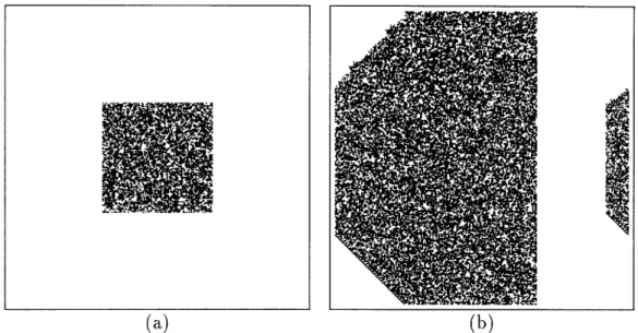
Figure 2-5 shows the behavior of a typical (i.e., random) rule that uses the von Neumann neighborhood (n = 5) and has one bit per cell (k = 2). The lookup table therefore consists of 25 = 32 bits. For this example, the table was created by generating a 32-bit random number: 2209261910 (written here in base 10). The initial condition is a 96x96 square of 50% randomness in which each cell has been independently initialized to 1 with a probability of 50% (0 otherwise). The resulting
(a) (b)
Figure 2-5: Typical behavior of a rule whose lookup table has been chosen at random. Starting from a block of randomness (a), the static spreads at almost the maximum possible speed (b).
disturbance expands at nearly the speed of light,3 and after 100 steps, it can be seen wrapping around the space. Note that the disturbance does not propagate to the right, which means that the rule doesn't depend on the left neighbor if there is a background of O's. Furthermore, the interior of the expanding disturbance appears to be just as random as the initial square. As a final comment, it can be verified by finding a state with two predecessors that this CA is indeed irreversible, as are most
CA.
Reversible rules can also display chaotic behavior, and in some sense, they must. The initial state of a system constitutes a certain amount of disorder, and since the dynamics is reversible, the information about this initial state must be "remembered" throughout the evolution. However, if the dynamics is nontrivial and there are not too many conservation laws, this information will get folded in with itself many times and the apparent disorder will increase. In other words, the entropy will increase, and there is a "second law of thermodynamics" at work.4 Figure 2-6 shows how
3The causal nature of CA implies that a cell can only be effected by perturbations in its
neighbor-hood on a single time step. The speed of light is a term commonly used to refer to the corresponding maximum speed of information flow.
4The notion of entropy being used here will be discussed in more detail in the next chapter.
I.'
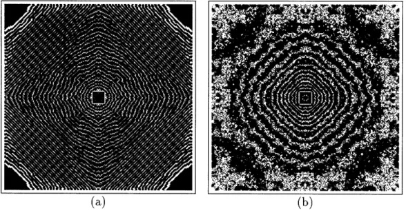
Figure 2-6: Typical behavior of a simple, symmetrical, reversible rule. Starting from a small, isolated, solid block (not shown), waves propagate outward and interfere with each other nonlinearly as they wrap around the space several times (a). After twice the time, the waves continue to become noiser and longer in wavelength (b).
this folding takes place and how the disorder typically increases in the context of a simple, nonlinear, reversible (second-order) rule. Initially, the system contained a solid 16 x 16 square (whose outline is still visible) in an empty background: obviously, a highly ordered state. Waves start to emanate from the central block, and after 1200 steps, the nonlinear interactions have created several noisy patches. After another 1200 steps, the picture appears even noiser, though certain features persist. The resulting bands of gray shift outward every step, and constitute superluminal phase waves (or beats) stemming from correlated information which has spread throughout the system.
2.3.2 Voting Rules
The dynamics of many CA can be described as a voting process where a cell tends to take on the values of its neighbors, or in some circumstances, opposing values [93]. Voting rules are characteristically irreversible because the information in a cell is often erased without contributing to another cell, and irreversibility is equivalent to destroying information. In practice, it is usually pretty clear when a rule is irreversible
lr
because frozen or organized states appear when there were none to begin with, and this means there must have been a many-to-one mapping of states. As we shall see, voting rules are examples of pattern-forming rules.
The first two examples in this section use a standard CA format called the Moore neighborhood which consists of a cell along with its nearest and next nearest neigh-bors: i. As before, the dot marks the cell which depends on the neighborhood, and the neighborhoods of nearby cells will overlap. The third example uses the other standard format, the von Neumann neighborhood.
We begin our survey of CA models with the most well-known example which is Conway's game of life. It was originally motivated as an abstract model of birth and death processes and is very reminiscent of cells in a Petri dish. While not strictly a voting rule, it is similar in that it depends on the total count of living cells surrounding a site (here, 1 indicates a living cell, and 0 indicates a dead cell or empty site). If an empty site has exactly 3 living neighbors, there is a birth. If a living cell has fewer than 2 or more than 4 living neighbors, it dies of loneliness or overcrowding respectively. All other cases remain unchanged. Figure 2-7(a) shows the default CAM-6 pattern of 50% randomness which is used as a standard in many of the examples below. Starting from this initial condition for 300 steps (with a trace of the activity taken for the last 100 steps) yields figure 2-7(b). The result is a number of stable structures, oscillating "blinkers," propagating "gliders," and still other areas churning with activity. It has been shown that this rule is already sufficiently complex to simulate any digital computation [4].
Figure 2-8 shows the behavior of some true voting rules with simple yes (1)/no (0) voting. Pattern (a) is the result of a simulation where each cell votes to go along with a simple majority (5 out of 9) of its neighbors. Starting from the standard random configuration and running for 35 steps gives a stable pattern of voters. At this point the rule is modified so that the outcome is inverted in the case of 4 or 5 votes. This has the effect of destabilizing the boundaries and effectively generating a surface tension. Figure 2-8(b) compares the system 200 and 400 steps after the rule is changed and shows how the boundaries anneal according to their curvature. The self-similar scaling
(a) (b)
Figure 2-7: Conway's game of life. The initial condition (a) is the standard pattern of randomness used in many of the examples below. After a few hundred steps (b),
complex structures have spontaneously formed. The shaded areas indicate regions of the most recent activity.
of the patterns is evident.
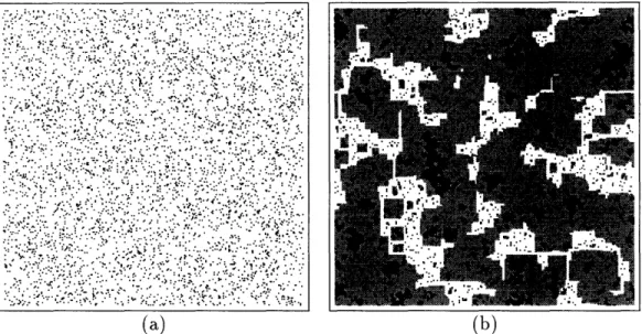
The final example of a voting rule is also our first example of a stochastic CA. The rule is for each cell to take on the value of one of its four nearest neighbors at random. Two bits from a chaotic CA (not shown) are used to pick the direction, and two bits of state specify one of four values in a cell. Since the new value of a cell always comes from a neighbor, the system actually decouples into two separate systems in a checkerboard fashion. Figure 2-9 shows how this dynamics evolves from a standard random pattern. After 1000 steps, the clustering of cell values is well underway, and after 10000 steps, even larger domains have developed. The domains typically grow according to power laws, _ t/ 2 where a < 1, and in an infinite space,
they would eventually become distributed over all size scales [18]. This rule has also been suggested as a model of genetic drift, where each cell represents an individual, and the value in the cell represents one of four possible genotypes [50].
3-i.I.E.
.
i~~~~~~~~~~~~~~~~~i~~~~~~~~~~~~~~~~~t~~~~~~~~~~~~~~~~~
(a) (b)
Figure 2-8: Deterministic voting rules. Starting from the standard random pattern, simple majority voting quickly leads to stable voting blocks (a). By having the voters vacillate in close elections, the boundaries are destabilized and contract as if under
surface tension (b). The shaded areas indicate former boundaries.
(a) (b)
Figure 2-9: A random voting rule with four candidates. Starting from a random mix of the four possible cell values, each cell votes to go along with one of its four nearest neighbors at random. After 1000 rounds of voting (a), distinct voting blocks are visible. After 10000 rounds (b), some regions have grown at the expense of others.
2.3.3 Reversible Rules
This section discusses a class of reversible CA that are based on second order rules, i.e., the next state depends on two consecutive time steps instead of only one. They use standard neighborhood formats, but the dynamical laws are all of the form st+l =
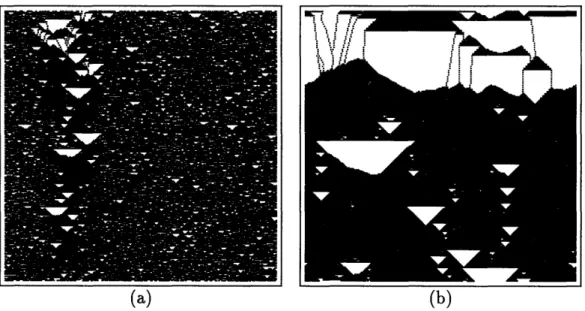
f({st) - t-1, where st denotes the state of a cell at time t, f({s}t) is any function of the cells in its neighborhood at time t, and subtraction is taken modulo an integer. Clearly this is reversible because st-l = f({st}) - st+l (in fact, it is time-reversal invariant). The example of a reversible chaotic rule in section 2.3.1 was also of this form, but the examples given here are more well-behaved due to the presence of special conservation laws. Another class of reversible rules based on partitioning neighborhoods will be discussed in the next section.
Figure 2-10 shows the behavior of a one-dimensional, second-order reversible rule with a neighborhood five cells wide. This particular rule has a (positive) conserved energy which is given by the number of differences between the current and past values of neighboring cells. The dynamics supports a wide variety of propagating structures which spread from regions of disorder into regions of order. Any deterministic CA on a finite space must eventually enter a cycle because it will eventually run out of new states. If in addition the rule is reversible, the system must eventually return to its initial state because each state can only have one predecessor. Usually the recurrence time is astronomical because there are so many variables and few conservation laws, but for the specific system shown in figure 2-10, the period is a mere 40926 steps.
Cellular automata are well-suited for doing dynamical simulations of Ising mod-els [19, 20, 93], where each cell contains one spin (1 = up, -1 = down). Many variations are possible, and figure 2-11 shows one such model that is a reversible, second-order CA which conserves the usual Ising Hamiltonian,
H=-J
sisj,
(2.1)
<i,j>
where J is a coupling constant, and < ... > indicates a sum over nearest neighbors. The second-order dynamics uses a so-called "checkerboard" updating scheme, where
Figure 2-10: A spacetime diagram of a one-dimensional, second-order rule in which conservation laws keep the system from exploding into chaos. Several kinds of prop-agating "particles," "bound states," and interactions are apparent.
the the black and red squares represent even and odd time steps respectively, so only half of the cells can change on any one step. The easiest way to describe the rule on one sublattice is to say that a spin is flipped if and only if it conserves energy, i.e., it has exactly two neighbors with spin up and two with spin down. The initial condition is a pattern of 8% randomness, which makes the value of H near the critical value. The spins can only start flipping where two dots are close enough to be in the von Neumann neighborhood of another cell, but after 10000 steps, fairly large patches of the minority phase have evolved. A separate irreversible dynamics records a history of the evolution (shown as shaded areas).
The energy in the Ising model above resides entirely in the boundaries between the phases, and it flows as a locally conserved quantity. It is not surprising then, that it is possible to describe the dynamics in terms of an equivalent (nonlinear) dynamics on the corresponding bond-energy variables. These energy variables form closed loops around the magnetic domains, and as long as the loops don't touch-and thereby interact nonlinearly-they happen to obey the one-dimensional wave equation in the plane of the CA. This wave behavior is captured in a modified form by the second-order, reversible CA in figure 2-12. The initial condition consists of of several normal
(a) (b)
Figure 2-11: A reversible, microcanonical simulation of an Ising model. The initial state has 8% of the spins up at random giving the system a near-critical energy (a). After roughly one relaxation time, the spins have aligned to form some fairly large magnetic domains (b). The shaded areas mark all the sites where the domains have been.
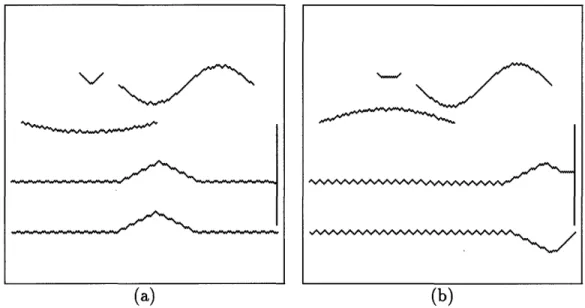
modes and two pulses traveling to the right on a pair of strings. All of the kinks in the strings travel right or left at one cell per time step, and therefore the frequency of oscillation of the normal modes is given by v = 1/A. The rule also supports open and closed boundary conditions, so the pulses may or may not be inverted upon reflection depending on the impedance. This rule is especially interesting in that it contains a linear dynamics in a nonlinear rule and illustrates how a field amplitude can be represented by the positions of particles in the plane of the CA.
2.3.4 Lattice Gases
The most important CA for physics, and those of the greatest current interest, are
the lattice gases. Their primary characteristic is that they have distinct, conserved
particles, and in most cases of interest, the particles have a conserved momentum. Lattice gases are characteristically reversible, though sometimes strict reversibility is violated in practice. The Ising bond-energy variable dynamics alluded to above, as well as many other CA, can be thought of as non-momentum conserving lattices
· '· ·'' 1··; ,.., . ' :-.::·· · ·r;=. C ' ' ''..'' '·' .··.·· · · ,:.: ?·· · : L I: ··J···`'::·· .· · i · :i; · · ·': 3··'· · · · · ' : ' : '· ..s··. :. .. I ·: .·r '''' -I-'·v · I · ·. ·\ · i : i .:· · · '" Y · TI ,,·;· · ·. 'by:Y : ·:- '.: .: :.: · · ·. j:5 .. :I Y. : .r I-'' · · '' · : ·. - · · · · ' · ·i ''' i: .... ·· i ·· · c 5% '· '.···' -I ··:... r"·' ·.·I.i'·:· :· ' :·I Y. · · r, .. "' :"''" :.: ::..: "I :.'...:: .I. :i s · ·: · ' :: .... " ·. c' '..-' C .'r . i.·:_ : i'''" /·· · · .c'' r·'· · · · · - · ·· : ::I i::: .. ',r . t,,r ':r "' '.'·' r''· · - · ·r·: "' .. r· :-... ;r,.· ·c· ·. ·- , :.:-··;.: · I'." .'.'?· :·-`::;···· .. ;1 · '·. '· i" "' .·I'' 'I .r··I
(a) (b)
Figure 2-12: A reversible, two-dimensional rule which simulates the one-dimensional wave equation in the plane of the CA. An initial condition showing normal modes as well as localized pulses (a). After 138 steps, the modes are out of phase, and the pulses have undergone reflection (b).
gases.5 However, for our purposes, lattice gases will be reversible and momentum conserving unless stated otherwise.
The rules in this section (and in the following section) use a partitioning CA format called the Margolus neighborhood: [E. In this case, all of the cells in the neighborhood depend on all of the others, and distinct neighborhoods don't overlap, i.e., they partition the space. This is very important because it makes it easy to make reversible rules which conserve particle number. One merely has to enforce reversibility and particle conservation on a single partition and these constraints will also hold globally. The cells in different partitions are coupled together by redrawing the partitions between steps (see for example, figures 2-2(b) and 3-4). Thus, the dynamical laws in a partitioning CA depend on both space and time.
The simplest example of a nontrivial lattice gas that one can imagine is the HPP lattice gas which contains identical, single-speed particles moving on a Cartesian lattice. The only interactions are head-on, binary collisions in which particles are deflected through 90°. Note that this is a highly nonlinear interaction (consider
5In fact, the term lattice gas originally referred to the energy variables of the Ising model.
US?
_EVLCYI_
(a) (b)
Figure 2-13: A primitive lattice gas (HPP) which exhibits several interesting phe-nomena. A wave impinging on a region of high index of refraction (a). The wave undergoes reflection as well as refraction (b).
the particles separately). One result of this (reversible) dynamics is to damp out inhomogeneities in the gas, and this dissipation can be viewed as an inevitable increase of entropy. Unfortunately, isotropic fluid flow is spoiled by spurious conservation laws such as the conserved momentum along each and every coordinate line. However, the speed of sound is a constant, 1/V2, independent of direction.
Figure 2-13 shows an implementation of the HPP model including an interesting modification. Here, the particles move diagonally, and horizontal and vertical "soli-ton" waves can propagate without dissipation at a speed of 1/v/2. These waves are maintained as a result of a moving invariant in which the number of particles along a moving line is conserved. The shaded area marks a region where the HPP rule operates only half the time. This effectively makes a lens with an index of refraction of n = 2, and there is an associated impedance mismatch. When the wave hits the lens, both a reflected and refracted wave result.
A better lattice gas (FHP) is obtained by switching to a triangular lattice and adding three-body collisions. This breaks the spurious conservation laws and gives a fully isotropic viscosity tensor. In the appropriate limit, one correctly recovers the incompressible Navier-Stokes equations. It is difficult to demonstrate hydrodynamic
(a) (b)
Figure 2-14: A sophisticated lattice gas (FHP) which supports realistic hydrodynam-ics. An initial condition with a vacuum surrounded by gas in equilibrium (a). The resulting rarefaction moves away at the speed of sound (b). The asymmetry is due to the embedding of the triangular lattice in a square one.
effects on CAM-6, but sound waves can be readily observed. Figure 2-14 shows an equilibrated gas with a 48x48 square removed. The speed of sound is again 1/V/2 in all directions, and after 100 steps, the disturbance has traveled approximately 71 lattice spacings. The wave appears elliptical because the triangular lattice has been stretched by a factor of vX2 along the diagonal in order to fit it into the Cartesian space of the machine.
2.3.5 Material Transport
Complex phenomena often involve the dissipative transport of large amounts of par-ticulate matter (such as molecules, ions, sand, or even living organisms); furthermore, CA are well-suited to modeling the movement and deposition of particles and the sub-sequent growth of patterns. This section gives two examples of CA which are abstract models of such transport phenomena. The models are similar to lattice gases in that they have conserved particles, but they differ in that they are characteristically irre-versible and don't have a conserved momentum. In order to conserve particles, it is again useful to use partitioning neighborhoods.
(a) (b)
Figure 2-15: A stylized model of packing sand. Shortly after starting from a near-critical density configuration, most of the material has stabilized except for a single expanding cave-in (a). Eventually, the collapse envelopes the entire system and leaves large caverns within densely packed material (b).
The detailed growth of materials depends on the mode of transport of the raw ma-terials. One such mode would be directed ballistic motion which occurs, for example, in deposition by molecular-beam epitaxy. Consideration of the action of gravity leads to abstract models for the packing of particulate material as shown in figure 2-15. The rule has been designed so that particles slide down steep slopes and fall straight down when there are no particles on either side. The result of this dynamics is the annealing of small voids and the formation of large ones. Eventually the system set-tles into a situation where a ceiling extends across the entire space. This model also exhibits some interesting "critical" phenomena. If the initial condition is denser than about 69%, the system rapidly settles down to a spongy state. If the initial density is less than about 13%, all of the particles end up falling continuously.
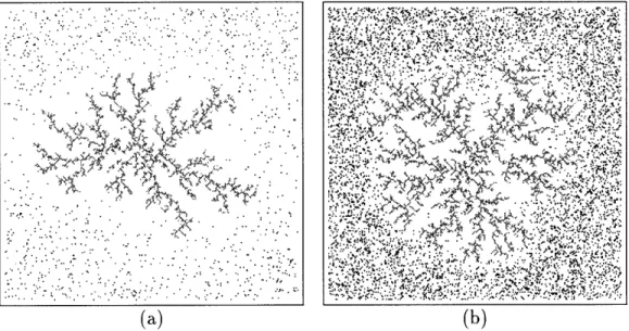
Another important mode of transport of small particles is diffusion. Figure 2-16 shows a model of diffusion limited aggregation in which randomly diffusing particles stick to a growing dendritic cluster. The cluster starts out with a single seed, and the initial density of diffusing particles is adjustable. The cluster in 2-16(a) took 10000 steps to grow in a gas with an initial density of 6%. However, with an initial density of 17%, the cluster in 2-16(b) formed in only 1000 steps. Fractal patterns such as
(a) (b)
Figure 2-16: A simulation of diffusion limited aggregation. Diffusing particles pref-erentially stick to the tips of a growing dendritic cluster (a). With a higher density of random walkers, the growth is more rapid and the cluster has a higher fractal dimension (b).
these are actually fairly commonly in dissipative CA models. While new abstract physical mechanisms would have to be constructed, the visual appearance of these patterns suggests the possibility of making CA models of crystal formation, electrical discharge, and erosion.
2.3.6 Excitable Media
A characteristic feature of a broad class of CA models is the existence of attractive, excitable states in which a cell is ready to "fire" in response to some external stimulus. Once a cell fires, it starts to make its way back to an excitable state again. The triggering stimulus is derived from a standard CA neighborhood, and the dynamics is characteristically irreversible. Such rules are similar to the voting rules in that the cells tend to follow the behavior of their neighbors, but they are different in that the excitations do not persist. Rather, the cells must be restored to their rest state during a recovery period. The examples given here differ from each other in the recovery mechanism and in the form of the stimulus. Like many of the irreversible CA above, they form patterns, but unlike the ones above, the patterns must oscillate. Many
:I :. · ·. r.·· .····.·: I-·:'-,·: ... . " .. ·':::`.,· .Y. :;· z--·· · c :·5 ... ·: : · I ·r .-· ... :I.V· .
r. r'.. ",: 1. ''~~~~~~~~~~~~~~'4
4;
"
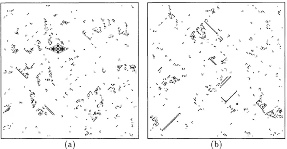
~ . II ., ..-. -..-. , ..-...-...-. -. (a) :. ' 4 : . .11 .LC. - .· (b)Figure 2-17: A model of neural activity in which cells must undergo a refractory
period after being stimulated to fire. Starting from the standard random pattern, the
system quickly settles down to a low density of complex, propagating excitations (a). After only 100 more steps, the pattern has completely changed (b).
models of excitable media are biological in nature, and even the game of life could perhaps be moved to this category.
The best example of excitable media found in nature is undoubtedly brain tissue, since very subtle stimuli can result in profound patterns of activity. At the risk of
drastically oversimplifying the real situation, neural cells have the property that they
fire as a result of activity in neighboring cells, and then they must rest for a short time before they can fire again. This behavior can be readily captured in a simple CA. A cell in the resting phase fires if there are exactly two active cells (out of 8) in its neighborhood. A cell which has just fired must wait at least one step before it can fire again. Figure 2-17 shows the behavior of this rule 100 and 200 steps after starting from the standard random pattern. The system changes rapidly and often has brief blooms of activity, though the overall level fluctuates between about two and three percent. This rule was specifically designed to prevent stationary structures, and it is notable for the variety of complex patterns it produces.
Many physically interesting systems consist of a spatially-distributed array or field of coupled oscillators. A visually striking instance of such a situation is given by the oscillatory Zhabotinsky redox reaction, in which a solution cycles through a series of
:.;|to .: - -.
, -:" .- .t..;:S
- . r:.. .. ~ */;
-·. , ' =:~:Z . : V ,"
.
/-.. , .:.S _ : o ·o .., x , · R : ~~~~~~~~~~~: v I : .,:.~..,~~'~.
-. ?
:,~.
~
. J'~If - r: ·i: 5; h r, .-.. C' ,. :i :·68 ": .·.···. -C ·' 1.(a) (b)
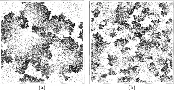
Figure 2-18: A model of oscillatory chemical reactions. When enough reactants are in the neighborhood of a cell, the next product in the cycle is formed. With a low reaction threshold, the resulting patterns are small, and the oscillations fall into a short cycle (a). A non-monotonic threshold creates large patterns which continually change (b).
chemical species in a definite order. Since there must be enough reactants present to go from one species to the next, the oscillators try to become phase locked by waiting for their neighbors. In a small reaction vessel, the solution will oscillate synchronously, but in a large vessel, some regions may be out of phase with the rest; furthermore, there may be topological constraints which prevent the whole system from ever becoming synchronized. Figure 2-18 shows two CA simulations of this phenomenon with different reaction thresholds. The resulting spiral patterns are a splendid example of self-organization. Similar phase locked oscillations can also be observed in fireflies, certain marine animals, and groups of people clapping.
The final example of an excitable CA is a stochastic predator-prey model. The fact that there are tens-of-thousands of degrees of freedom arranged in a two-dimensional space means that the behavior cannot be captured by a simple pair of equations. The prey reproduce at random into empty neighboring cells, while the predators reproduce into neighboring cells that contain prey. Restoration of the empty cells is accomplished by having the predators randomly die off at a constant rate. Figure 2-19 shows the behavior of this dynamics for two different death rates. Variations on this