Greedy Randomized Search Procedure to Sort Genomes using Symmetric, Almost-Symmetric and Unitary Inversions

HAL Id: hal-00922670

https://hal.inria.fr/hal-00922670

Submitted on 4 Jul 2017

HAL is a multi-disciplinary open access

archive for the deposit and dissemination of

sci-entific research documents, whether they are

pub-lished or not. The documents may come from

teaching and research institutions in France or

abroad, or from public or private research centers.

L’archive ouverte pluridisciplinaire HAL, est

destinée au dépôt et à la diffusion de documents

scientifiques de niveau recherche, publiés ou non,

émanant des établissements d’enseignement et de

recherche français ou étrangers, des laboratoires

publics ou privés.

Greedy Randomized Search Procedure to Sort Genomes

using Symmetric, Almost-Symmetric and Unitary

Inversions

Ulisses Dias, Christian Baudet, Zanoni Dias

To cite this version:

Ulisses Dias, Christian Baudet, Zanoni Dias. Greedy Randomized Search Procedure to Sort Genomes

using Symmetric, Almost-Symmetric and Unitary Inversions. Proceedings of the 4th ACM

Confer-ence on Bioinformatics, Computational Biology and Biomedical Informatics (ACM BCB 2013), ACM

Special Interest Group on Bioinformatics, Computational Biology, and Biomedical Informatics, Sep

2013, Maryland, United States. pp.181–190, �10.1145/2506583.2506614�. �hal-00922670�

Greedy Randomized Search Procedure to Sort Genomes

using Symmetric, Almost-Symmetric and Unitary

Inversions

Ulisses Dias

udias@ic.unicamp.br

Christian Baudet

Lyon, France

christian.baudet@

univ-lyon1.fr

Zanoni Dias

zanoni@ic.unicamp.br

ABSTRACT

Genome Rearrangement is a field that addresses the prob-lem of finding the minimum number of global operations that transform one given genome into another. In this work we develop an algorithm for three constrained versions of the event called inversion, which occurs when a chromosome breaks at two locations called breakpoints and the DNA be-tween the breakpoints is reversed. The constrained versions are called symmetric, almost-symmetric and unitary inver-sions. In this paper, we present a greedy randomized search procedure to find the minimum number of such operations between two genomes. Our approach is, to our knowledge, the first genome rearrangement problem modeled using this metaheuristic. Our model is an iterative process in which each iteration receives a feasible solution whose neighbor-hood is investigated for a better solution. This search uses greediness to shape the candidate list and randomness to se-lect elements from the list. A previous greedy heuristic was used as an initial solution. In almost every case, we were able to improve that initial solution by providing a new sequence of inversions that uses less operations. For permutations of size 10, our solutions were, on average, 5 inversions shorter than the initial solution. For permutations of size 15 and 20, our solutions were, on average, 10 and 16 inversions shorter than the initial solution, respectively. For longer permuta-tions ranging from 25 to 50 elements, we generated solupermuta-tions that were, on average, 20–22 inversions shorter than the ini-tial solution. We believe that the method proposed in this work can be adjusted to other genome rearrangement prob-lems.

General Terms

Algorithm

Keywords

GRASP, genome rearrangement, symmetric inversion

1.

INTRODUCTION

Greedy randomized search procedures have been routinely used as metaheuristics to find solutions for combinatorial optimization problems that are close to the optimal solu-tion. This metaheuristic was first introduced by Feo and Resende [16], who described how to use a randomized ap-proach for the set cover problem. They used the acronym GRASP (Greedy Randomized Adaptive Search Procedure) to identify the procedure.

GRASP has been applied to several NP-hard problems such as the 2-partition [17], 2-layer straight line crossing minimization [24], matrix decomposition [27], job schedul-ing [1], proportional symbol maps [8] and Steiner problem in graphs [28], to name a few. The reader is referred to the review written by Festa and Resende [18] for a more detailed discussion about GRASP.

In this paper, we present a greedy randomized search pro-cedure to sort genomes using symmetric, almost-symmetric and unitary inversions. This is, to our knowledge, the first genome rearrangement problem modeled using this approach. We believe other problems in the genome rearrangement field could also make use of GRASP. For example, the sort-ing by transpositions problem and the sortsort-ing by prefix-inversions problem which were recently settled as NP-hard [6, 7] have several greedy approaches that could be randomized, some of these approaches were used to deviate algorithms with approximation guarantee [4, 15, 19].

Assuming a minimization problem written as “min f (x) for x ∈ X”, where f is an objective function to be mini-mized and X is a discrete set of feasible solutions, GRASP searches for good solutions as an iterative process. Each it-eration uses an initial solution x0∈ X, and its neighborhood

is investigated until a local minimum is found. Our approach follows this model and also implements other basic compo-nents of GRASP as described by Feo and Resende [16].

Section 2 is a brief introduction to the problem. It pro-vides the concepts and definitions used throughout the text.

Section 3 presents our search procedure. The section is self-contained, and we assume no previous knowledge about the concepts of GRASP. Section 4 analyses the model using a practical approach. We base our analysis on the improve-ment that was achieved by our model when a previous greedy approach is used as an initial solution [10].

2. GENOME REARRANGEMENT

Genome rearrangements are large-scale mutations that af-fect large stretches of DNA sequence in a genome. Several rearrangement events have been proposed in the past two decades. Among these events, inversions were established as the main explanation for the genomic divergence in a va-riety of organisms such as insect [13], plant [3, 21, 26], mam-mal [20, 22], virus [29], and bacteria [9].

An inversion occurs when a chromosome breaks at two lo-cations called breakpoints and the DNA between the break-points is reversed. This genome rearrangement event led to the problem of sorting by inversions, which is to find the minimum number of inversions that transform one genome into another. Hannenhalli and Pevzner [21] presented the first polynomial algorithm for this problem, which was later simplified by Bergeron [5]. Tannier and Sagot [30] presented an algorithm that runs in sub-quadratic time.

In some families of bacteria, an ‘X’-pattern is observed when two circular chromosomes are aligned [11,14]. We have been studying this pattern among members of the Pseu-domonadaceae family and the Mycobacterium, Xanthomonas and Shewanella genera [11]. Figure 1 shows one example of genome alignment for members of the Pseudomonadaceae family where the ‘X’-pattern can be clearly seen.

0 1000000 2000000 3000000 4000000 5000000 6000000 0 1000000 2000000 3000000 4000000 5000000

Pseudomonas syringae pv B728a

Pseudomonas entomophila L48

Figure 1: MUMmer [23] pairwise alignment of

Pseudomonadaceae chromosomes. Dots represent

matches between the chromosome sequences. Red dots depict matches in the same orientation in both chromosomes, whereas blue dots depict matches in opposite orientation. The dots form a clear ‘X’-pattern.

Inversions that are symmetric to the origin of replication (meaning that the breakpoints are equally distant from the origin of replication) have been proposed as the primary mechanism that explains the ‘X’-pattern [14]. The justifi-cation relies on the fact that one single highly asymmetric inversion affecting a large area of the genome could destroy the ‘X’-pattern, even though short inversions are still possi-ble. Another study using Yersinia genomes [9] has added ev-idence that such symmetric inversions are “over-represented”

with respect to other types of inversions.

Figure 2 shows a simplified scenario where a set of inver-sions acts on an ancestral genome. The ancestral genome evolves in a 2-branch scenario and symmetric inversions oc-cur on both branches. Assuming both pairs (A1, B1), and

(A2, B2) represent contemporary species, it would be

possi-ble to spot the ‘X’-pattern when aligning their genomes. Only few works take symmetry in consideration. Ohle-busch et al. [25] use symmetric inversion to compute an ancestral genome (the so-called median problem). Dias et al. [12] proposed the problem of sorting genomes using only symmetric or almost-symmetric inversions. Recently, Dias and Dias [10] added unitary inversions to the problem, thus creating the problem of sorting permutations using symmet-ric, almost-symmetric or unitary inversions.

They presented a greedy sorting heuristic based on an ex-tension of the cycle graph [4, 21], which is a tool used to handle several genome rearrangement problems. The exten-sion is based on assigning weights to a subset of edges in the graph. We will use this extension to create our greedy randomized approach.

2.1

Definitions

In the literature on genome rearrangement that focuses on mathematical models of genomes, a chromosome is usually represented as a permutation π = (π1π2. . . πn), for πi∈ I,

1≤ |πi| ≤ n, and i ̸= j ↔ |πi| ̸= |πj|. Each πi represents

a gene (or others markers), and that gene is assumed to be shared by the genomes being compared, with n being the total number of genes shared.

Here we consider a permutation as a bijective function in the set{−n, . . . , −2, −1, 1, 2, . . . , n} such that π(i) = πiand

π(−i) = −π(i).

The composition of two permutations π and σ is the per-mutation π· σ = (πσ(1) πσ(2) . . . πσ(n)). We can see the

composition as the relabeling of elements in π according to elements in σ. Let ι be the identity permutation ι(i) = i, we can easily verify that ι is a neutral element such that π· ι = ι · π = π.

We define the inverse of a permutation π as the permu-tation π−1 such that π· π−1 _{= π}−1_{· π = ι. The inverse}

permutation is the function such that π_π(i)−1 = i. In other words, it is the function that returns the position in π of each element πi.

An inversion is an operation in which the order of a per-mutation segment is inverted. As a consequence, the signs of the elements in the inverted segment are also changed.

Formally, the inversion denoted by ρ(i, j) is the permuta-tion (1 . . . i− 1 − j − (j − 1) . . . − (i + 1) − i j + 1 . . . n), 1≤ i ≤ j ≤ n. Thus, applying an inversion to a permu-tation π is the the same as the composition π· ρ(i, j) = (π1, . . . , πi−1,−πj,−πj−1, . . . ,−πi+1,−πi, πj+1, . . . , πn).

In this work, we allow three kinds of operations to sort a permutation: symmetric inversions, almost-symmetric in-versions and unitary inin-versions. We defined these inin-versions as follows:

Symmetric Inversion ρ is an inversion around the ori-gin of replication such that ρ(i) = ρ(i + 1, n− i), 0≤ i ≤ ⌊n−1

2 ⌋. Figure 3(a) exemplifies the symmetric

inversion.

Almost-Symmetric Inversion !ρ is an inversion around the origin of replication such thatρ(i, j) = ρ(i + 1, n! −

0 0 0 0 0 0 0 0 0 0 −18 1 1 −18 ₁ 1 1 2 2 ₂ 2 2 2 −17 3 3 3 3 2 2 3 −17 4 4 −16 4 −16 4 −15 5 5 −14 −14 4 −15 5 6 4 −14 4 6 6 −13 4 −13 5 −12 7 7 6 7 −13 7 7 −12 8 8 8 6 8 6 6 8 9 ₉ 9 8 8 9 9 9 9 8 8 8 10 10 10 10 10 10 10 11 11 11 11 11 11 10 10 10 11 12 12 −7 12 12 −7 −6 −6 12 13 13 13 14 14 13 12 14 −5 12 −6 −5 12 15 15 −5 15 14 15 −4 16 16 16 15 −4 16 16 17 17 17 −3 17 14 14 −3 14 17 −2 −2 18 18 18 18 18 16 −1 −1 16 16 18 18 18 0 0 2 4 6 8 10 12 14 16 18 0 2 4 6 8 10 12 14 16 18 2 4 6 8 10 12 14 16 18 B2 B1 B0 B2 A1 A2 A0 A1 A0 _A2 B0 B1 Common Ancestor

Figure 2: Explanation for the ‘X’-pattern as proposed by Eisen et al. [14]. Each inversion occurs between two bullets (•). Numbers represent the order of genes or other markers. Dots in the dotplots represent matches between the chromosome sequences. Red dots depict matches in the same orientation in both chromosomes, whereas blue dots depict matches in the opposite orientation. The dotplots begin to resemble the actual dotplot like that present in Figure 1 after just a few symmetric operations.

j), 0≤ i, j ≤ n − 1, |i − j| = 1. Figure 3(b) exemplifies the almost-symmetric inversion.

Unitary Inversion ˙ρ is an inversion affecting one single element of the permutation such that ˙ρ(i) = ρ(i, i), 1≤ i≤ n. Figure 3(c) exemplifies the unitary inversion. In genome rearrangement problems, the goal is to find a minimum number of operations ρ1, ρ2, . . . , ρm, ρi∈ {ρ, !ρ, ˙ρ}

that lead from one permutation π to another permutation σ. In other words, we want to find a sequence of permutations S =< S0, S1, . . . , Sm >, such that S0 = π, Sm = σ, and

Si= Si−1· ρi.

It is important to highlight that the sequence ρ1, ρ2, . . . , ρm

is the same that would be used to transform σ−1· π into ι, that is because we can easily relabel the entire sequence S using the composition in order to create the sequence S′_=<

σ−1· S0, σ−1· S1, . . . , σ−1· Sm>, where σ−1· S0= σ−1· π

and σ−1· Sm = σ−1· σ = ι. This property will be useful

later to create our greedy randomized search procedure (see Functions 1 and 2 in Algorithm 1).

The cycle graph is a tool used to handle several genome re-arrangement problems [4,21]. We defined a cycle graph G(π) of a permutation π as follows: the vertex set is{−n, . . . , −2, −1, 1, 2, . . . , n} ∪ {0, −(n + 1)}. Two set of edges can be de-fined: the gray edge set is{+(i − 1), −i}, for 1 ≤ i ≤ n + 1, and the black edge set is{−πi, +πi−1}, for 1 ≤ i ≤ n + 1.

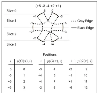
The permutation π = (+5−3 −4 +2 +1) generates the ver-tex set {0, −5, +5, +3, −3, +4, −4, −2, +2, −1, +1, −6} and the edge sets shown in Figure 4.

We define the slice of each vertex i in G(π) as the function slice(G(π), i) = min{|π−1_{(i)|, n − |π}−1_{(i)| + 1} for i in the}

set{−n, . . . , −2, −1, 1, 2, . . . , n}. Otherwise, for i = 0 or i = −(n+1), we define slice(G(π), i) = 0. Figure 4 indicates the slice for each vertex in the cycle graph for π = (+5 − 3 − 4

+2 +1).

We define the position of each vertex i in G(π) as the function: p(G(π), i) = ⎧ ⎪ ⎪ ⎨ ⎪ ⎪ ⎩ 0 if i = 0 2n if i =−(n + 1) 2|π−1(i)| − 1 if π−1(i) < 0 2|π−1_{(i)| if π}−1_{(i) > 0}

For the permutation π = (+5 − 3 − 4 +2 +1), we show the position p(G(π), i) of each element i in Figure 4.

We say that an inversion ρ(a, b) acts on vertex i of G(π) if 2a− 1 ≤ p(G(π), i) ≤ 2b + 1. Moreover, we say that an inversion acts on a gray edge (i, j) if it acts on either i or j. Dias and Dias [10] extended the cycle graph structure by assigning a weight w(G(π), i, j) to each gray edge. They define two approaches for the weight assignment. The first approach was defined as the minimum number of symmetric, almost-symmetric or unitary inversions that should act on the gray edge (i, j) in order to create a black edge (j, i).

The second approach adds the new constraint that these inversions should only act on the vertex placed in the higher slice. Moreover, if slice(G(π), i) = slice(G(π), j), then the inversions should only act on one vertex.

Figure 5 exemplifies both approaches. Figure 5(a) is the first approach. The first inversion acts on i and j, bringing them close to each other, this inversion would not be allowed by the second approach. Figure 5(b) is the case when the vertex i should not be moved (since i is in the lowest slice). We can see a longer path to create the black edge (j, i).

We tested both approaches using only a small set of in-stances and we came to the conclusion that the second ap-proach fits better to our heuristic than the first one. There-fore, for a gray edge (i, j) we assign a weight w(G(π), i, j) using the second approach.

O -7 -2 +1 -5 -3 +4 -6 -8 ⇐ O -7 -2 +1 +3 +5 +4 +8 +6 (3,6)

(a) Symmetric Inversion

O -7 -3 +1 +2 -6 +4 -8 -5 ⇐ O -7 -2 +1 +3 +5 +4 +8 +6 (3,7) (b) Almost-Symmetric Inversion ⇐ O -7 -2 +1 +3 +5 +4 +8 +6 (3,3) O -7 -2 +1 -3 +5 +4 +8 +6 (c) Unitary Inversion

Figure 3: Allowed inversions.

3. GREEDY RANDOMIZED SEARCH

PRO-CEDURE

Our method works by iteratively improving a sorting se-quence of permutations. Each step requires a local change in order to find a better (shorter) solution. If a shorter se-quence is found, it is made the current solution. We repeat this step until a solution regarded as optimal is found or the iteration limit is reached.

The initial solution for local search is generated by a previ-ous greedy heuristic [10]. The heuristic constructs a solution one element at a time. Each step gathers a set of candi-date permutations that can be added to extend the partial solution. The selected permutation is the one which mini-mizes the greedy function h1(π) = min{w(G(π), i, −(i+1)),

w(G(π), n−i−1, −(n−i))}+w(G(π), i, −(i+1)) + w(G(π), n− i − 1, −(n − i)), for 1 ≤ i ≤ ⌈n

2⌉.

The function h1 favours elements in lower slices. Let

(+5 -3 -4 +2 +1) 0 -6 +5 -5 -3 +3 -4 +4 +2 -2 +1 -1 Gray Edge Black Edge Slice 0 Slice 1 Slice 2 Slice 3 Positions p(G(π), i) i -5 +5 +3 -3 +4 1 2 3 4 5 p(G(π), i) i -4 -2 7 8 p(G(π), i) i +2 -1 +1 9 10 11 -6 12 0 0

Figure 4: Cycle graph G(π) for π = (+5 − 3 − 4 +2 +1). We also indicate the slice and position for each vertex in the graph.

i j i j i j ji i j 2 i j ji ₀

(a) First approach

(b) Second approach

2 1 ₀

3

1

Figure 5: Example of weights being assigned to gray edges (i, j). In a) we compute the minimum number of operations to create the black edge (j, i), and in b) we further restrict to allow only those inversions acting on the vertex placed in the higher slice if they are in different slices, otherwise we allow only inversions acting on one of the two vertices.

(i1, j1) and (i2, j2) be two gray edges, min{slice(G(ι), i1),

slice(G(ι), j1)} < min{slice(G(ι), i2), slice(G(ι), j2)}. The

function promotes the formation of a black edge (j1, i1)

be-fore the black edge (j2, i2). Besides, the black edge (j1, i1)

will not be cut when attempting to create the black edge (j2, i2). As a result, the function h1 guarantees a feasible

solution for any input permutation.

The drawback of using the greedy algorithm to find an initial solution for local search is that we start from the same solution every time. We could repeatedly start our local search from randomly generated solutions in order to overcome this problem. However, the average quality of the random solutions would be much worse than that of the greedy algorithm. Furthermore, the number of iterations it takes to converge in these cases would be larger than when the greedy initial solution is used, which also impacts the overall running time.

The next two sections explain our method. Section 3.1 explains our algorithm main structure, but will not provide details about the local search mechanism. Those details will be provided in Section 3.2.

3.1 Algorithm Structure

Let S =< S0, S1, . . . , Sm > be a sequence of

permuta-tions where Si= Si−1· ρ, 1 ≤ i ≤ m, ρ ∈ {ρ, !ρ, ˙ρ}, S0is the

input permutation, and Sm= ι. Our local search method

attempts to build a shorter feasible solution using S as a starting point. In this phase, the neighborhood of S is in-vestigated by using greediness to shape the candidate list and randomness to select elements from the list.

We say that a solution X is in the neighborhood of S in re-gard to a sequence of anchor permutations P =< P0, P1, . . . ,

Pl>, namely X∈ N(S, P ), if for each Pi∈ P , then Pi∈ S

and Pi∈ X. Moreover, let S−1(Pi) and X−1(Pi) be the

po-sition of Piin S and X, respectively. For each pair Pi, Pj,

i < j, then S−1_(P

i) < S−1(Pj) and X−1(Pi) < X−1(Pj). It

is worth noticing that P must have at least two elements: P0= π0and Pl= ι.

Algorithm 1 shows our Greedy Randomized Search Pro-cedure to improve the initial solution. Starting from the solution S, each iteration produces a sample of solutions sample(S), sample(S) ⊆ N(S, P ). Section 4 will explain how the anchor point set P will be created. For now, we take P for granted.

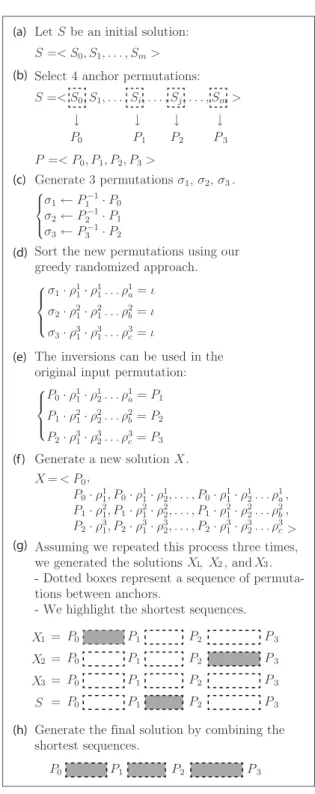
Some concepts we present might be difficult to compre-hend. Thus we summarize the main steps in Figure 6. We will refer to this figure when new concepts are presented.

The sample(S) set is restricted to a fixed number of ele-ments given by the parameter Sample_Size in Algorithm 1. The more elements used, the larger the variance in the set. In Figure 6, we restrict the sample(S) set to 3 elements.

After we populate the sample(S) set, we combine the el-ements in the search for the best solution (lines 6 – 9).

To create the sample(S) set we investigate the neighbor-hood N (S, P ) in the following way:

1. Each pair Pi−1, Pi, 1≤ i ≤ l is used to create a new

permutation σi= Pi−1· Pi−1(line 14). In Figure 6(b)

we selected 4 anchor permutations. In this case, we were able to create σ1, σ2 and σ3 in Figure 6(c).

2. We sort each σiusing a greedy randomized approach

shown in Function 2 of Algorithm 1. Some details about this function will be provided in Section 3.2. For now, we only need to know that this function re-turns a list of operations ρi

1, ρi2, . . . , ρia such that σi·

ρi1· ρi2. . . ρia= ι.

3. For each permutation Pi, we apply the list of

opera-tions obtained from sorting σi. That list transforms Pi

into the permutation Pi+1as we can see in Figure 6(e).

In Algorithm 1, this step is performed from line 13 to line 19.

4. After applying the previous steps for each pair Pi,

Pi−1, 1≤ i < l, we join the small sequences to make

a solution as we show in Figure 6(f). We repeat the entire procedure in order to obtain the desired number of solutions.

5. When sample(S) is fully populated, we combine the elements in the set sample(S)∪ {S} to create the best

Let S be an initial solution: S =< S0, S1, . . . , Sm> Select 4 anchor permutations: S =< S0, S1, . . . , Si, . . . , Sj, . . . , Sm> P =< P0, P1, P2, P3> Generate 3 permutations σ1, σ2, σ3. ⎧ ⎪ ⎨ ⎪ ⎩ σ1← P1−1· P0 σ2← P2−1· P1 σ3← P3−1· P2

Sort the new permutations using our greedy randomized approach.

σ1· ρ11· ρ11. . . ρ1a= ι σ2· ρ21· ρ21. . . ρ2b= ι σ3· ρ31· ρ31. . . ρ3c= ι

The inversions can be used in the original input permutation:

P0· ρ11· ρ12. . . ρ1a= P1 P1· ρ21· ρ22. . . ρ2b= P2 P2· ρ31· ρ32. . . ρ3c= P3 Generate a new solution . X = < 0 P0· ρ11, P0· ρ11· ρ21, . . . , P0· ρ11· ρ12. . . ρ1a P1· ρ21, P1· ρ21· ρ22, . . . , P1· ρ21· ρ22. . . ρ2b P2· ρ31, P2· ρ31· ρ23, . . . , P2· ρ31· ρ32. . . ρ3c> ← P0 P1 P2 P3 ← ← ← ⎧ ⎪ ⎨ ⎪ ⎩ ⎧ ⎪ ⎨ ⎪ ⎩ , , , P (a) (b) (c) (d) (e) (f) (g) (h) X

Assuming we repeated this process three times, we generated the solutions , , and . - Dotted boxes represent a sequence of permuta-tions between anchors.

- We highlight the shortest sequences. 1 2 3 X X X P0 P1 P2 P3 1 X = P0 P1 P2 P3 2 X = P0 P1 P2 P3 3 X = P0 P1 P2 P3 S = P0 P1 P2 P3

Generate the final solution by combining the shortest sequences.

Figure 6: Example of local search. S is the initial solution whose neighborhood will be investigated and P is the anchor permutation sequence. We set |P | = 4. Assuming we generate 3 solutions for each iteration, we will combine them with the initial so-lution in the search for a best soso-lution.

Algorithm 1: Greedy Randomized Search Procedure 1 Data: π, S, M ax Iterations, Sample Size, Anchors 2 Solution← Greedy Construction(π)

3 for k = 1, . . . , M ax Iterations do

4 sample← ∅

5 P←Select Anchor Points(S, Anchors) 6 for k = 1, . . . , Sample Size do

7 Solution←Build Solution(P )

8 sample.append(Solution)

9 S←Combine(sample ∪ {S}, P ) 10 return S

11Function 1: Build Solution 12 Data: P

solution← [] 13 for i = 1, . . . , |P | do 14 σ← Pi−1· Pi−1 15 aux← Pi−1

16 operations←Greedy Randomized Local Search(sigma)

17 for each operation in operations do

18 solution.append(aux)

19 aux← aux · operation

20 return solution

21Function 2: Greedy Randomized Local Search 22 Data: σ

23 operations← [] 24 _{while σ ̸= ι do} 25 scores← []

26 for each ρ applicable to σ, ρ ∈ {ρ,!ρ, ˙ρ} do 27 score←Score Permutation(σ · ρ) 28 scores.append([score, ρ]) 29 scores.sort(f irst elements)

30 scores← scores[0 . . . 5] // Select five elements starting from the first one 31 selected←Roulette Wheel Selection(scores) 32 ρ← scores[selected][1]

33 σ← σ · ρ

34 operations.append(ρ) 35 return operations

36Function 3: Roulette Wheel Selection 37 Data: scores

38 F itness ← [scores[0][0], 0, 0, 0, 0, 0] 39 i ← 1

40 while i < 5 do

41 F itness[i] ← F itness[i − 1] + scores[i][0]

42 i ← i + 1 43 R ← random(0, F itness[5]) 44 i ← 0 45 while R > F itness[i] do 46 i ← i + 1 47 return i

48Function 4: Score Permutation 49 Data: σ

50 score ← 0 51 i ← 0 52 while i ≤ |σ| do

53 score← score + w(G(σ), i, −(i + 1), 2)

54 i ← i + 1

55 return score2

solution (line 9). We overlook the details of this func-tion because it is simple. In summary, we select the shortest sequence starting from Piand ending at Pi+1

in some solution, for 1≤ i < l. Then, we simply cre-ate a new solution joining the sub-sequences. In this phase, it is possible that the best solution is equal to S. In Figure 6(g), we have three solutions in sample(S). We combine those solutions and the initial solution S by retrieving the highlighted dotted boxes, which represent the shortest sequence between two given an-chors. After that, we join these sequences (boxes) to create a final solution.

3.2

Local Search

In this section we explain how a solution in the neigh-borhood of S is generated. Each permutation σistarts the

construction of a sorting sequence one element at a time. The next permutation to be added to the solution must be approved in a two-step process:

1. The next permutation must be ranked as high as fifth by the greedy function h(σ) = (&|σ|_i=0w(G(σ), i,−(i + 1)))2_{. This function is the square of the sum of all gray}

edge weights in the cycle graph of the permutation. We use the sum of the gray edge weights because it indicates how far we are from the identity permuta-tion. In fact,&|ι|_i=0w(G(ι), i,−(i + 1))) = 0, which is a desirable property for a greedy function.

We use the square in the h(σ) function because a small difference in the sum of weights usually indicates a big difference in the quality of the candidate permutation. Since the next step uses randomness to select one of the 5 candidates, we would like to better distinguish good candidates from bad candidates.

In Algorithm 1, this step is carried out by Function 4 that goes from line 48 to line 55.

2. The next permutation to be added to the solution must be selected by a random process called roulette wheel selection mechanism, which is very common in Genetic Algorithm techniques [2].

In the roulette wheel selection mechanism, each per-mutation has a selection likelihood proportional to its greedy score. This step is implemented in Function 3 that goes from line 36 to line 47. This function receives the score array as a parameter and stores the cumula-tive sum in the F itness array, which provides tempo-rary working storage. After that, a random number R is generated in the range defined by the F itness array. Finally, we select the first element in the set such that when all previous greedy scores are added it gives us at least R.

4.

RESULTS

We have implemented Algorithm 1 in python. The run-ning time becomes prohibitive unless we find a tradeoff be-tween the parameters M ax Iterations and Sample Size. In this test we set the parameters M ax Iterations = 1000, and Sample Size = 1. Since Algorithm 1 uses a random-ized approach, each run can return a different value. For this reason, we run each input 10 times and plot the results.

Line 5 in Algorithm 1 calls the function “Select Anchor Points” that still needs to be further explained. This func-tion creates a sequence P =< P0, P1, . . . , Pl >, where P0

is the input permutation and Pl = ι. We want to assess

how the size |P | impacts our results. Therefore, we ran the same input permutation with four different sizes for P : |P | ∈ {2, 3, 4, 5}.

One important consideration is that we want all the sub-sequences < Pi, . . . , Pi+1 >, i ≤ 0 < l, in the current

so-lution to have approximately the same length. It is also important to mention that the choice of the anchor permu-tations must be randomized, because if we do not randomize the choice, we will probably select the same permutation Pi

every time. If Pi is not in any optimal sorting of the

in-put permutation, we will never be able to find an optimal solution.

We implemented Algorithm 2 taking these requirements in consideration. In summary, we choose a point by random in the range '(|S|₃ ). . .*2|S|₃ +,, then we use this point to create roughly balanced anchor points, depending on the number of anchor points requested.

Algorithm 2: Select Anchor Points 1 Data: S, Anchor P oints

2 if Anchor P oints = 2 then 3 return [S0, ι]

4 if Anchor P oints = 3 then 5 choice← random((|S|3

) ,*2|S|₃ +) 6 return [S0, Schoice, ι]

7 if Anchor P oints = 4 then 8 choice ← random((|S|3 ) ,*2|S|₃ +) 9 lef t ←-2choice 3 . 10 right ←(2choice+|S|3 ) 11 return [S0, Slef t, Sright, ι]

12 if Anchor P oints = 5 then 13 choice ← random((|S|3 ) ,*2|S|₃ +) 14 lef t ←-choice 2 . 15 right ←(choice+|S|2 )

16 return [S0, Slef t, Schoice, Sright, ι]

The main quality measure used in our experiments is the difference in size between the sequence produced by our im-plementation and the initial solution produced by the greedy approach.

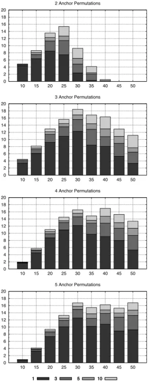
For n in the set{10, 15, . . . , 50}, we generated 100 random permutations and ran our implementation of Algorithm 1 on them. Figure 7 shows how often our approach improves the greedy approach solution. We were able to improve the result of almost every input permutation using some anchor point schema, which shows that it is generally worth running our greedy randomized approach after a greedy solution is built.

Another conclusion we take from Figure 7 is that we should increase the number of anchors for larger permutations. For n = 10, we can improve the greedy initial solution in 96% of the cases by using only 2 anchors, which was the best we could get in our experiment for this permutation length.

0 10 20 30 40 50 60 70 80 90 100 10 15 20 25 30 35 40 45 50 2 Anchor Permutations 0 10 20 30 40 50 60 70 80 90 100 10 15 20 25 30 35 40 45 50 3 Anchor Permutations 1 3 5 10 0 10 20 30 40 50 60 70 80 90 100 10 15 20 25 30 35 40 45 50 4 Anchor Permutations 1 3 5 10 0 10 20 30 40 50 60 70 80 90 100 10 15 20 25 30 35 40 45 50 5 Anchor Permutations 1 3 5 10

Figure 7: Permutations whose initial solutions were improved using our method. Y-axis represents the percentage of improved solution in the database. X-axis represents permutation size. Each plot uses a different set of anchor points. In each plot, we indi-cate whether the improvement was obtained in the 1st, 3rd, 5th or 10th run.

However, the solution quality of the 2 anchor version de-grades when n grows. In this case, increasing the number of anchor permutations is appropriate.

The histograms for the 3, 4, and 5 anchor versions confirm this idea. Note that each one was good for a particular range of permutation length. For example, the 2 anchor version did a good job for n in the range [10..20]. The 3 anchor version was appropriate for n in the range [15..35]. The 4 and 5 anchors version had 100% of improvement in the range [20..30] and similar number of improvements in the range [35..45]. However, for n = 50, the 5 anchor version is the best choice.

Later we show a relation between the size of the sorting sequence and the preferred number of anchors. The larger the size of the initial solution, the more anchors we need.

Figure 8 shows the improvement on average obtained by using our method. Let S be the initial solution and Sfbe the

final solution produced by our greedy randomized approach. We define improvement as the difference in size between Sf

and S. For n = 10, 2 anchors were better than the others, providing solutions that were 4.88 elements smaller than the initial greedy solution. By using 3, 4 and 5 anchors we were able to improve, on average, 4.36, 1.93 and 0.90 elements, respectively. These values are consistent with our previous idea that few anchors are more appropriate for small per-mutations.

From n = 15 to n = 20, the 2 anchor version kept the best performance, but it achieved lower results for n≥ 25. For 25 ≤ n ≤ 35, the 3 anchor version returned the best results, but for n = 35, both the 4 and 5 anchor versions closed the range. For n = 40, the 3 anchor version provided solutions that were 16.34 elements smaller than the initial solution (on average). The 4 anchor versions improved the original solution by an average of 16.97 elements. Although it is a small difference between both versions, this can be described as an intersection point.

The intersection point between the 4 and 5 anchor version was detected when n = 45, but the difference was very small. For n = 50, the 5 anchor version was clearly better than any of the others with an average of 16.78, against an average of 13.39 for the 4 anchor version and 11.18 for the 3 anchor version. The 2 anchor version did not improve any initial solution for n = 50.

The results above were obtained by running each version independently of each other. Figure 9 shows the average im-provement when considering all 4 anchors versions together. Although the results are better here than in Figure 8, the difference is small. Thus, the decision whether to run the method several times with different numbers of anchors is left to the user.

To assist in this decision, in Figure 10 we arrange our data in a different way. In this plot, we assess how our method behaves when we change the number of anchors for different initial sequence sizes. As expected, we can see that for higher initial sequences we should favour choosing more anchor permutations.

Let m be the number of elements in the initial sequence, we can see that for 10 ≤ m ≤ 70 the 2 anchor version presents the best results on average. For 70≤ m ≤ 130 the 3 anchor version is much better than any of the others. For 130 ≤ m ≤ 190 there is a tie between the 4 and 5 anchor version, but a slight advantage can bee seen in favour of the 4 anchor version. In this range we suggest using both

0 2 4 6 8 10 12 14 16 18 20 10 15 20 25 30 35 40 45 50 2 Anchor Permutations 0 2 4 6 8 10 12 14 16 18 20 10 15 20 25 30 35 40 45 50 3 Anchor Permutations 1 3 5 10 0 2 4 6 8 10 12 14 16 18 20 10 15 20 25 30 35 40 45 50 4 Anchor Permutations 1 3 5 10 0 2 4 6 8 10 12 14 16 18 20 10 15 20 25 30 35 40 45 50 5 Anchor Permutations 1 3 5 10

Figure 8: Average improvement obtained by using our method. Y-axis represents an average of the difference in size between the sequence produced by our implementation and the initial sequence. X-axis represents permutation size. Each plot uses a differ-ent set of anchor points. In each plot, we indicate whether the improvement was obtained in the 1st, 3rd, 5th or 10th run.

0 2 4 6 8 10 12 14 16 18 20 [10..40) [40..70) [70..100) [100..130) [130..160) [160..190) [190..220) [220..250) Average Improvement

Initial Sequence Length

2 Anchors 3 Anchors 4 Anchors 5 Anchors

Figure 10: Average improvement obtained by using our method. Y-axis represents an average of the difference in size between the sequence produced by each version of our implementation and the initial sequence. X-axis represents the size of initial greedy sequence.

0 2 4 6 8 10 12 14 16 18 20 22 24 10 15 20 25 30 35 40 45 50 1 3 5 10

Figure 9: Average improvement when considering all 4 anchor versions. Y-axis represents an aver-age of the difference in size between the sequence produced by our implementation and the initial se-quence. X-axis represents permutation size. Each plot uses a different set of anchor points. In each plot, we indicate whether the improvement was ob-tained in the 1st, 3rd, 5th or 10th run.

approaches. For 190 ≤ m ≤ 250 the 5 anchor version has clearly the best performance.

5. CONCLUSION

In this paper we presented a greedy randomized search procedure to the problem of finding the minimum number of symmetric, almost-symmetric and unitary inversions that transform one given genome into another. Our method is to our knowledge the first genome rearrangement problem modeled using that metaheuristic. We believe this method can be adjusted to other genome rearrangement problems.

Our model is an iterative process in which each iteration receives a feasible solution whose neighborhood is

investi-gated for a better solution. This search uses greediness to shape the candidate list and randomness to select elements from the list.

In order to use our method, it is necessary to provide an initial solution and to set three parameters. We use a pre-vious greedy heuristic as initial solution. The parameters can be easily set and tuned. Two of them, M ax Iterations and Sample Size, impact the time spent processing the re-sult. In our case, a tradeoff between them was reached by using a small set of instances. The last parameter defines the number of anchor permutations we use in each iteration. This parameter impacts the quality of the solution provided by our method. We made an extensive analysis in order to find the best configuration to this parameter according to the size of the input permutation and the size of the initial solution. By this analysis, we give some insights on how to properly set the parameter.

We were able to improve the initial solution in almost every case during our experiments. For permutations of size 10, our solutions were on average 5 inversions shorter than the initial solution. For permutations of size 15 and 20, our solutions were on average 10 and 16 inversions shorter than the initial solution, respectively. For longer permutations ranging from 25 to 50 elements, we generated solutions that were on average 20–22 inversions shorter than the initial solution.

6.

ACKNOWLEDGMENTS

This work was made possible by a Postdoctoral Fellowship from FAPESP to UD (number 2012/01584-3), by project funding from CNPq to ZD (number 477692/2012-5), and by French Project ANR MIRI BLAN08-1335497 and the ERC Advanced Grant SISYPHE to CB. FAPESP and CNPq are Brazilian funding agencies.

The authors thank Espa¸co da Escrita - Coordenadoria Geral da Universidade - UNICAMP - for the language ser-vices provided.

7. REFERENCES

[1] R. M. Aiex, S. Binato, and M. G. C. Resende. Parallel grasp with path-relinking for job shop scheduling. Parallel Computing, 29:2003, 2002.

[2] T. B¨ack. Evolutionary algorithms in theory and practice: evolution strategies, evolutionary

programming, genetic algorithms. Oxford University Press, Oxford, UK, 1996.

[3] V. Bafna and P. A. Pevzner. Sorting by reversals: Genome rearrangements in plant organelles and evolutionary history of X chromosome. Molecular Biology and Evolution, 12(2):239–246, 1995. [4] V. Bafna and P. A. Pevzner. Sorting by

transpositions. SIAM Journal on Discrete Mathematics, 11(2):224–240, 1998.

[5] A. Bergeron. A very elementary presentation of the Hannenhalli-Pevzner theory. Discrete Applied Mathematics, 146:134–145, 2005.

[6] L. Bulteau, G. Fertin, and I. Rusu. Pancake flipping is hard. In Mathematical Foundations of Computer Science 2012, volume 7464 of Lecture Notes in Computer Science, pages 247–258. 2012. [7] L. Bulteau, G. Fertin, and U. Rusu. Sorting by

transpositions is difficult. In Automata, Languages and Programming, volume 6755 of Lecture Notes in Computer Science, pages 654–665. 2011.

[8] R. G. Cano, G. Kunigami, C. C. Souza, and P. J. Rezende. A hybrid grasp heuristic to construct effective drawings of proportional symbol maps. Computers and Operations Research, 40(5):1435 – 1447, 2013.

[9] A. E. Darling, I. Mikl´os, and M. A. Ragan. Dynamics of genome rearrangement in bacterial populations. PLoS Genetics, 4(7):e1000128, 2008.

[10] U. Dias and Z. Dias. Sorting genomes using

symmetric, almost-symmetric and unitary inversions. In Proceedings of the 5th International Conference on Bioinformatics and Computational Biology

(BICoB’2013), pages 261 – 268, Honolulu, USA, 2013. [11] U. Dias, Z. Dias, and J. C. Setubal. A simulation tool

for the study of symmetric inversions in bacterial genomes. In Comparative Genomics, volume 6398 of Lecture Notes in Computer Science, pages 240–251. 2011.

[12] Z. Dias, U. Dias, J. C. Setubal, and L. S. Heath. Sorting genomes using almost-symmetric inversions. In Proceedings of the 27th Symposium On Applied Computing (SAC’2012), pages 1–7, Riva del Garda, Italy, 2012.

[13] T. Dobzhansky and A. H. Sturtevant. Inversions in the third chromosome of wild races of Drosophila pseudoobscura, and their use in the study of the history of the species. Proceedings of the National Academy of Science, 22:448–450, 1936.

[14] J. A. Eisen, J. F. Heidelberg, O. White, and S. L. Salzberg. Evidence for symmetric chromosomal inversions around the replication origin in bacteria. Genome Biology, 1(6):research0011.1–0011.9, 2000. [15] I. Elias and T. Hartmn. A 1.375-approximation

algorithm for sorting by transpositions. IEEE/ACM Transactions on Computational Biology and Bioinformatics, 3(4):369–379, 2006.

[16] T. Feo and M. G. C. Resende. Greedy randomized adaptive search procedures. Journal of Global Optimization, 6(2):109–133, 1995.

[17] T. A. Feo and M. Pardalos. A greedy randomized adaptive search procedure for the 2-partition problem. Operations Research, 1994.

[18] P. Festa and M. Resende. Grasp: basic components and enhancements. Telecommunication Systems, 46(3):253–271, 2011.

[19] J. Fischer and S. W. Ginzinger. A 2-approximation algorithm for sorting by prefix reversals. In

Proceedings of the 13th Annual European Symposium on Algorithms (ESA’2005), pages 415–425, Mallorca, Spain, 2005. Springer-Verlag.

[20] S. Hannenhalli and P. A. Pevzner. Transforming Men into Mice (Polynomial Algorithm for Genomic Distance Problem). In Proceedings of the 36th Annual Symposium on Foundations of Computer Science (FOCS’95), pages 581–592, Los Alamitos, USA, 1995. [21] S. Hannenhalli and P. A. Pevzner. Transforming

cabbage into turnip: polynomial algorithm for sorting signed permutations by reversals. Journal of the ACM, 46(1):1–27, 1999.

[22] J. D. Kececioglu and R. Ravi. Of Mice and Men: Algorithms for Evolutionary Distances Between Genomes with Translocation. In Proceedings of the 6th Annual Symposium on Discrete Algorithms, pages 604–613, New York, USA, 1995.

[23] S. Kurtz, A. Phillippy, A. L. Delcher, M. Smoot, M. Shumway, C. Antonescu, and S. L. Salzberg. Versatile and open software for comparing large genomes. Genome Biology, 5(2):R12, 2004.

[24] M. Laguna and R. Mart´ı. Grasp and path relinking for 2-layer straight line crossing minimization. INFORMS Journal on Computing, 11:44–52, 1999.

[25] E. Ohlebusch, M. I. Abouelhoda, K. Hockel, and J. Stallkamp. The median problem for the reversal distance in circular bacterial genomes. In Proceedings of the 16th Annual Symposium on Combinatorial Pattern Matching (CPM’2005), pages 116–127, Jeju Island, Korea, 2005.

[26] J. D. Palmer and L. A. Herbon. Plant mitochondrial DNA evolves rapidly in structure, but slowly in sequence. Journal of Molecular Evolution, 27:87–97, 1988.

[27] M. Prais and C. C. Ribeiro. Reactive grasp: An application to a matrix decomposition problem in tdma traffic assignment. INFORMS Journal on Computing, 12:164–176, 1998.

[28] C. C. Ribeiro, E. Uchoa, and R. F. Werneck. A hybrid grasp with perturbations for the steiner problem in graphs. INFORMS Journal on Computing, 14:200–2, 2001.

[29] C. Rooney, N. Taylor, J. Countryman, H. Jenson, J. Kolman, and G. Miller. Genome rearrangements activate the epstein-barr virus gene whose product disrupts latency. Proc Natl Acad Sci USA, 85(24):9801–5, 1988.

[30] E. Tannier and M.-F. Sagot. Sorting by reversals in subquadratic time. In Proceedings of the 15th Annual Symposium on Combinatorial Pattern Matching (CPM’2004), pages 1–13, Istambul, Turkey, 2004.