Modal Trajectory Estimation using Maximum Gaussian Mixture

HAL Id: hal-02917190

https://hal.archives-ouvertes.fr/hal-02917190

Submitted on 18 Aug 2020

HAL is a multi-disciplinary open access

archive for the deposit and dissemination of

sci-entific research documents, whether they are

pub-lished or not. The documents may come from

teaching and research institutions in France or

abroad, or from public or private research centers.

L’archive ouverte pluridisciplinaire HAL, est

destinée au dépôt et à la diffusion de documents

scientifiques de niveau recherche, publiés ou non,

émanant des établissements d’enseignement et de

recherche français ou étrangers, des laboratoires

publics ou privés.

Modal Trajectory Estimation using Maximum Gaussian

Mixture

André Monin

To cite this version:

André Monin. Modal Trajectory Estimation using Maximum Gaussian Mixture. IEEE Transactions

on Automatic Control, Institute of Electrical and Electronics Engineers, 2013, 58 (3), pp.763 - 768.

�10.1109/TAC.2012.2211439�. �hal-02917190�

Modal Trajectory Estimation using Maximum

Gaussian Mixture

André Monin

CNRS, LAAS, 7 ave du Colonel Roche, F-31077 Toulouse, France.

Univ de Toulouse, LAAS, F-31400 Toulouse, France.

Abstract—This paper deals with the estimation of the whole

trajectory of a stochastic dynamic system with highest proba-bility, conditionally upon the past observation process, using a maximum Gaussian mixture. We first recall the Gaussian sum technique applied to minimum variance filtering. It is then shown that the same concept of Gaussian mixture can be applied in that context, provided we replace the Sum operator by the Max operator.

Index Terms—Filtering, Smoothing, Gaussian sum, Gaussian

mixture.

I. INTRODUCTION

The Gaussian mixture approximation introduced in [1] has become a very popular way to approximate many filtering issues. It is defined classically as a weighted sum of Gaussian probability density functions (pdf) as follows:

p (x) =

m

X

i=1

i (x xi; Pi)

where x_{2 R}n_{, and stands for the Gaussian pdf}

(x; P ) = p 1

(2 )n_{jP j}exp 1 2x

T_P 1_x

Nowadays, computation facilities are allowed to implement algorithms based on this approximation. Indeed, in practice, the computational load is equivalent to N Kalman Filters or Extended Kalman Filters (EKFs) in parallel. The value of N depends obviously on the application, but it rarely exceeds a few hundreds. In practice, it may be more efficient than the so-called particle filtering technique which often needs thousands of particles [2] (convergence rate of 1=pN versus 1=N for

deterministic algorithms).

Classically, the Gaussian mixture approximation consists of developing the transition or the observation pdf, or both, as weighted sums of Gaussian densities [1]. Such an approx-imation permits to deal, for example, with linear systems with non-Gaussian noises and/or non-Gaussian initial pdf, nonlinear systems with Gaussian noises but such that the standard deviation of noises is large with respect to the field of validity of the linearization [1], nonlinear systems with non-Gaussian white noises and multi-modal systems with Markovian commutations [3].

In this paper, the problem of the modal trajectory estima-tion (MTE) [4] is addressed. The goal is to find the whole

trajectory over the horizon [0; t] with the highest probability, conditionally upon the past observation process:

x_0:t= arg max

x0:t

p (x0:tjy0:t)

where x0:t, fx0; : : : ; xtg and y0:t, fy0; : : : ; ytg. Note that

the outcome x_t of the optimal trajectory x_0:t is, in general, not the same as the state obtained by maximizing the marginal density p (xtjy0:t), the Max a posteriori (MAP) filter, except

for the linear Gaussian case (the Kalman filter).

Curiously, there are only few studies on the MTE issue even if it is of real interest, specifically when the conditional probability is multi-modal. In [5], the author states the gen-eral problem and then limits itself to the Gaussian case. In [4], the authors address the general case using the dynamic programming approach, as we do, but limiting themselves to the regular case (all pdf are functions but not distributions).

Our main contribution is to show that the same concept of Gaussian mixture filters, first devoted to minimum variance filtering, occurs in the MTE issue provided by replacing the Sum operator by a Max operator (section III). First, we recall in section II-A how the marginal conditional density and in section II-B the marginal Bayesian likelihood propagate in the general Markovian case [4]. Both minimum variance and modal trajectory smoothers are derived using backward computations in the general case. We then show in section II-B that the MTE issue is in most cases ill-posed and then we suggest a solution to regularize this.

II. GENERAL MINIMUM VARIANCE AND MODAL TRAJECTORY ESTIMATES

The goal of general optimal filtering theory is to compute the estimate of the internal state xt 2 Rn of a stochastic

dynamic system partially observed by the process yt 2 Rp

over the interval [0; t]. Generally, the Markovian system model reduced to the transition pdf p (xtjxt 1) and the observation

pdf p (ytjxt). The optimal filtering concept refers to a

par-ticular criterion. There are two main criteria commonly used. The first one is the "minimum variance filter". This estimate is intended to minimize the expectation of the quadratic norm of the error between the process and its estimate, using only the past observations y0:t, that is

^ xtjt= arg min F( ) E h kxt F (y0:t)k2 i (1)

where _{F stands for any function of the observation process.} It leads to the expectation of the conditional pdf p (xtjy0:t):

^ xtjt=

Z

xtp (xtjy0:t) dxt (2)

The second one, named MTE, is intended to maximize the pdf of the state path x_0:t conditionally upon the output past, that is [6]:

x_0:t= arg max

x0:t

p (x0:tjy0:t)

Note that in most cases, only the outcome of the optimal trajectory x_t is of interest as the computation of the whole trajectory x ; < t needs a backward calculation which is not

generally computable in real-time (as it is the case with the minimum variance smoother ^x _{jt= E [x jy}0:t] with < t).

A. Minimum variance estimate

The pdf p (xtjy0:t) can be propagated using the following

theorem.

Theorem 1: Beginning with the knowledge of the initial pdf

p (x0) (a measurable function), the a posteriori pdf can be

computed recursively by:

p (xtjy0:t) = p (ytjxt) R p (xtjxt 1) p (xt 1jy0:t 1) dxt 1 R p (ytjxt) p (xtjy0:t 1) dxt (3) Proof: See [6].

Note that even if the transition pdf p (xtjxt 1) is a

distribu-tion, the pdf p (xtjy0:t) is in most cases a measurable function

due to the smoothing property of the integral operator. The filter can then be computed using 2.

This means that the general solution to optimal filtering, in the minimum variance sense, is achieved by recursively spreading one function of the state (the a posteriori pdf of the state) with one integration operation over the state space and one function multiplication.

With the knowledge of the set _{fp (x jy}0:t) ; = 0; : : : ; tg,

the whole optimal smoother ^x _{jt= E [x jy}0:t], < t can then

be computed backward using the following theorem.

Theorem 2: Beginning with the optimal filtering solution

p (xtjy0:t), the optimal smoother can be computed backward

as follows: _{8 = t} 1; : : : ; 0 p (x jy0:t) = p (x jy0: ) Z p (x +1jy0:t) R p (x +1jx ) p (x jy0: ) dx p (x +1jx ) dx +1 Proof: See [6].

B. Modal trajectory estimate

1) Regular case: Recall that the goal is to maximize the

pdf p (x0:tjy0:t). Assume that this pdf is a measurable function

(not a distribution). Using the Bayes rule, this density can be rewritten as

p (x0:tjy0:t) =

p (y0:tjx0:t) p (x0:t)

p (y0:t)

As the denominator does not depend on the variable to be optimized (x0:t), it is equivalent to maximizing the numerator

and then to compute

x_0:t= arg max

x0:t

J (x0:t; y0:t)

where

J (x0:t; y0:t), p (y0:tjx0:t) p (x0:t) (4)

As it is done dealing with dynamic programming, let us define the marginal Bayesian likelihood:

J_t(xt; y0:t), max x0:t 1

J (x0:t; y0:t) (5)

Again, this optimal marginal Bayesian likelihood can be computed recursively.

Theorem 3: Beginning with the knowledge of the initial

marginal Bayesian likelihood J₀(x0;y0) = p (y0jx0) p (x0) (a

measurable function), the optimal marginal maximum likeli-hood can be computed recursively by the following equation

J_t (xt; y0:t) = max xt 1

p (ytjxt) p (xtjxt 1) Jt 1(xt 1; y0:t 1)

(6)

Proof: See [4].

The outcome x_t of the optimal trajectory x_0:t can then be computed by

x_t = arg max

xt

J_t (xt; y0:t)

This means that the general solution to optimal filtering, in the MTE sense, is achieved recursively with one Max operation over the state space and one function multiplication. Note then the similarity between equations (3) and (6) where integration operator is just replaced by a Max operator.

With the knowledge of the set_{fJ (x ; y}0: ) ; = 0; : : : ; tg,

the whole optimal trajectory (the MTE smoother) can then be computed backward using the following theorem.

Theorem 4: The MTE x_0:t can be computed backward

according to

The outcome of the optimal trajectory is defined by

x_t = arg max

xt

J_t (xt; y0:t)

The whole optimal trajectory can be computed backward by_{8 = t} 1; : : : ; 0

x = arg max

x

p x _+1jx J (x ; y0: ) (7)

Proof: See [4].

2) Singular case: In most cases, the transition probability

measure has no measurable density. Indeed, the dynamic noise dimension is often less than the state dimension. For example, consider vehicle tracking model where only speed and course are noisy when position is a deterministic function of speed and course. In such a case, the MTE is ill-posed. Indeed, there is no mathematical sense to consider the maximization of measures. The problem has then to be regularized. Note that, to the knowledge of the author, this point has never been addressed in the literature (authors often consider, "for simplicity", that the covariance of the dynamic noise Q is a regular matrix [6] [5]).

In most practical cases, the state can be split into two parts [6]: the first one is deterministic with respect to the past (x(1)_{t 2 R}n1_{) and the second one is noisy (x}(2)

t 2 Rn2). In

these cases, the state representation takes the following form:

x(1)_t = f(1)(xt 1) (8a)

x(2)_t = f(2)(xt 1; wt) (8b)

where wtis the dynamic white noise such that p x(2)t jxt 1

is a measurable pdf (a function). The transition pdf is then replaced by a transition probability measure and takes then the following form:

P dx(1)t jxt 1 = f(1)_(x t 1) dx (1) t p x (2) t jxt 1 dx(2)t

where a(dx) stands for the Dirac measure at a. As the cost

defined by (4) is not a function but a measure, it is equivalent to consider the new joint likelihood as follows:

~ J (x0:t; y0:t), p (y0:tjx0:t) t Y =1 p x(2)_jx 1 p (x0) dx0 (9) adding the constraint set

8 = 1; : : : t; x(1)_{= f}(1)_(x

1) (10)

This modified optimal marginal likelihood defined by 9 can be then computed recursively using the following theorem.

Theorem 5: In the singular case, beginning with the

knowl-edge of the initial marginal likelihood

~

J₀(x0; y0), p (y0jx0) p (x0)

the optimal marginal maximum likelihood can be computed recursively by the following equation

~ J_t(xt; y0:t) = max xt 1; t 1 p (ytjxt) p x(2)t jxt 1 exp T_{t 1} x(1)_t f(1)(xt 1) ~ J_{t 1}(xt 1; y0:t 1) (11)

where t 1 2 Rn1 is a Lagrange multiplier related to the

constraint x(1)_t = f(1)(xt 1).

Proof: It is directly derived from classical maximization

under constraints using Lagrange multipliers. See [7] for details.

Again, with the knowledge of the set

fJ (x ; y0: ) ; = 0; : : : ; tg, the whole optimal trajectory

(the smoother) can then be computed backward.

Theorem 6: The whole MTE can be computed backward

according to

The outcome of the optimal trajectory is defined by

x_t = arg max

xt

~

J_t(xt; y0:t)

The whole optimal trajectory can be computed backward by _{8 = t} 1; : : : ; 0

x = arg max

x ;

p x(2)_+1jx (12)

exp T x(1)₊₁ f(1)(x ) J (x ; y~ 0: )

with the constraint x(1)₊₁= f(1)_{(x ).}

Proof: See [7].

III. MODAL TRAJECTORY ESTIMATE USINGGAUSSIAN MIXTURE

A. Gaussian mixture definition

For simplicity of presentation, only the linear non-Gaussian case is developed here. Moreover, we consider here the sin-gular case as it is the most common in practice. According to section II-B2, the state space is split into two components

x(1)_{t 2 R}n1 _{and x}(2)

t 2 Rn2. The transition of x (1) t is

deterministic and the transition of x(2)_t is defined by weighted point-wise maximization. Indeed, if one deals with a linear non Gaussian system, one can write

x(1)_t = F(1)xt 1

x(2)_t = F(2)_x

t 1+ wt

where the non Gaussian white noise pdf can be approximated as follows:

p (wt) = max i=1;:::;m

i _w

t wi; Qi

Indeed, it is easy to imagine that many pdf could be approx-imated by a point-wise Max of Gaussian pdfs as it is the case for the Sum of Gaussian pdfs [8]. As a consequence, the transition pdf can be written as:

p x(2)_{t jx}t 1 ' max i=1;:::;m

i _x(2)

t F(2)xt 1 wi; Qi

and where all Qi _{and R are assumed to be non-singular}

matrices.

This choice is motivated by our estimation scheme. Indeed, unlike the sum operator, the Max operator is distributive with itself and associative with multiplication by positive variable: _{8a; b; c} 0, max (c max (a; b)) = max (ac; bc) but max (c (a + b)) 6= max (ac; bc).

For simplicity of presentation with restrict ourselves to Gaussian observation pdf

p (ytjxt) ' (yt Hxt; R)

In fact, it is straightforward to generalize the observation pdf as a Gaussian mixture defined by

p (ytjxt) ' max j=1;:::;q

j _y

t Hxt vj; Rj

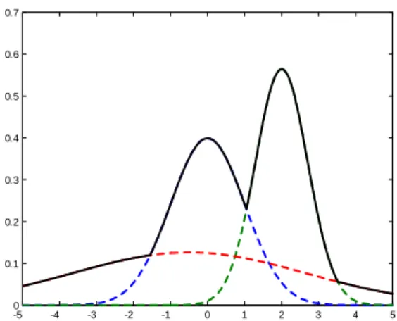
Figure 1 shows and example of such a Gaussian mixture.

B. Spreading the optimal marginal likelihood

Recall that the MTE requires the recursive computation of

~

Jt (xt; y0:t). We then have the following theorem:

Theorem 7: If at step t 1, the optimal marginal likelihood

can be written as a Gaussian mixture of Nt 1terms as follows:

J_{t 1}(xt 1; y0:t 1)

= max

k=1;::;Nt 1

k

-5 -4 -3 -2 -1 0 1 2 3 4 5 0 0.1 0.2 0.3 0.4 0.5 0.6 0.7

Fig. 1. Example of Gaussian mixture. The continuous black line represents the pointwise Max.

then, at step t, the marginal likelihood is again a Gaussian mixture with Nt= Nt 1 m q terms defined by

J_t(xt; y0:t) = max k=1;::;Nt 1 i=1;:::;m k;i t xt x^k;i_tjt; P_tk;i_jt where k;i t = kt 1 i r F(1)_Bk;i t F(1) T r (2 )n B_tk;i yt H ^xk;i_{tjt 1}; k;i_{tjt 1} B_tk;i = P_{t 1}k _{jt 1} S_tk;iF(2)P_{t 1}k _{jt 1} P_t(2);k;i_{jt 1} = F(2)P_{t 1}k _{jt 1} F(2) T + Qi S_tk;i = P_{t 1}k _{jt 1} F(2) T P_t(2);k;i_{jt 1} 1 ^ xk;i_t jt 1, " F(1)_x^k t 1jt 1 F(2)_x^k t 1jt 1+ wi # P_tk;i_{jt 1} = 2 6 4 F (1)_Bk;i t F(1) T+ F(1)S k;i t P (2);k;i tjt 1 S k;i t F(1)S k;i t T P_t(2);k;i_{jt 1} F(1)_Sk;i t T F(1)_Sk;i t P (2);k;i tjt 1 P_t(2);k;i jt 1 # (14) ^ xk;i_t jt = x^ k;i tjt 1+ K k;i t yt H ^xk;i_{tjt 1} (15a) k;i tjt 1 = HP k;i tjt 1H T _{+ R (15b)} K_tk;i = P_tk;i jt 1H T k;i tjt 1 1 (15c)

P_tk;i_jt = P_tk;i_{jt 1} K_tk;iP_tk;i_{jt 1}HT (15d)

Proof: See [7].

As it was the case for minimum variance filtering, the conditional pdf at time t is similar to those defined at t 1 but

the number of Gaussian pdfs grows exponentially with time as Nt = Nt 1 m q. In practice, it is clear that such a

filtering algorithm is not tractable. Many approximations have been proposed to reduce the exponential growing number of Gaussian pdfs. They mainly consist of maintaining only Nmax

pdfs, Nmax being the maximum number of Kalman filters

well-matched with the computational power allocated to the application. The most popular techniques are:

maintaining only the Nmax pdfs with highest weights,

pruning others and then scaling [9];

merging several Gaussian pdfs in one equivalent Gaussian pdf, according to some distance criterion, the new pdf having the same mean and variance as the Gaussian subset [1] [10] [11] [12] [13] [14] [15] [16] [17] [3] [18] [19].

If the conditional marginal likelihood is written at time t as follows

J_t (xt; y0:t) = max k=1;::;Nt

k

t xt x^ktjt; Ptkjt

then the outcome of the maximum likelihood trajectory is computed by first looking for the Gaussian indice that leads the maximum value J_t:

k = arg max k=1;::;Nt k t r (2 )n Pk tjt (16)

The optimal estimate is then the expectation of this Gaussian pdf: x_tjt = ^xk

tjt. Note that in our case, the Max value of

J_t (xt; y0:t) coincide exactly with the mean of one Gaussian

pdf (the k -th), unlike in the Gaussian sum approximation scheme [20].

C. Computing the modal trajectory estimate

The whole modal trajectory can be computed backward using the following theorem.

Theorem 8: The MTE over the interval [0; t] can be

com-puted backward as follows:

Computation of the outcome of the optimal trajectory x_t

jt

by 16.

Backward computation of the whole trajectory:_{8 = t}

1; : : : ; 0 (k ; i ) = arg max k=1;::;N i=1;:::;m 0 B B @ k i r F(1)_Bk;i _F(1) T r Bk;i x(2)₊₁ x^(2);k;i₊₁ j ; P (2);k;i +1j (17) x(1)₊₁ F(1) k;i_+1j ; F(1)B_{t 1}k;i F(1) T x = k ;i_+1j + Bk ;i F(1) T F(1)Bk ;i F(1) T 1 (18) x(1)₊₁ F(1) k ;i_+1j

where ^ x(2);k;i_+1j = F(2)x^k_j + wi (19a) P(2);k;i_+1j = F(2)Pk_j F(2) T+ Qi (19b) Sk;i_j = P(2);k;i_j F(2) T P(2);k;i_+1j 1 (19c) k;i +1j = x^ k j + S k;i j x (2) +1 x^ (2);k;i +1j (19d) Bk;i = Pk_j Pk_j F(2) T P(2);k;i_+1j 1F(2)Pk_j Proof: See [7].

Note that it is generally necessary to compute again ^xk;i_+1j ,

Pk;i_+1j and Bk;i _{because the number of Gaussian pdfs is}

reduced to N at each step with N +1 6= N m q in

practice. Moreover, note that one may be interested only by a sliding past horizon optimal trajectory limiting the backward computation_{8 = t 1; : : : ; t T where T stands for duration} of this past horizon.

Remark 9: Extension to the non linear case. Recall that

we have restricted ourselves to the linear non Gaussian case. If the dynamic and/or observation function are not linear, it is easy to extend this approach using classical approximations. Indeed, all computations made in this algorithm use classical Gaussian pdf multiplication formulae. In the non linear case, these products may be approximated using linearization [6] or unscented transformation [21], for example.

IV. SIMULATION RESULTS

The MTE algorithm has been tested with a simplified target tracking issue. Consider a target, for example a boat, with known speed (for simplicity) which can change its course at any time with an unknown rotation speed. Assume that the observer is static and has a remote access to the range rt (

accuracy of 10 m) and the azimuth angle t ( accuracy of

13 ) of the target. The state of the target can be defined by

the vector xt= [rt; t; t; !t] where t stands for the target

course and !tits rotation speed. The state equation may then

be defined as follows rt = rt 1+ V cos ( t t) t t = t 1+ V rt 1 sin ( _t t) t t = t 1+ !t 1 t

where V = 20knot stands for the target speed and t = 1 s

for the sampling period. The random deviation of the rotation speed can be depicted as a Markovian stochastic process as follows

p (!tj!t 1) /

max ( 0 (!t !t 1; Q0) ; 1 (!t !t 1; Q1) ; 2 (!t; Q2))

The first Gaussian density depicts the little drift of the rotation speed (pQ0 = 3 10 4 =s), the second Gaussian density

depicts a sudden change of the rotation speed (pQ1= 3 =s)

and the third Gaussian density depicts the back-pulling to a rotation speed close to zero (pQ2 = 3 10 4 =s). Thus, 1 stands for the mean of the target steerage frequency ( 1=

1=500 Hz) and 1= ₂for the mean of the steerage time (1= ₂= 60 s). In our scenario, the observer is located at the origin of a

Cartesian coordinate system. The initial location of the target is ( 1000 m; 1000 m). Its initial course is equal to 70 . After

60 s, the target starts a course steering fixing the rotation speed

to 3 =s. This steering stops 40 s later.

As the transition pdf is singular, we used the algorithm of theorem 7. We have compared the MAP using a Gaussian sum approximation and the MTE. More precisely, we have extended both algorithms to the nonlinear case by linearization (extended Kalman filter). Both algorithms use Nmax = 33

Gaussian pdfs to represent the a posteriori density p (xtjy0:t)

and the marginal maximum likelihood ~J_t (xt; y0:t). An

exam-ple of target location tracking is shown on figure 2 where the modal trajectory (the smoother) is computed backward according to theorem ??. The course tracking is illustrated on figure 3. -1200 -1000 -800 -600 -400 -200 0 200 500 600 700 800 900 1000 1100 1200 1300 m m Actual location MTE MAP Smoother

Fig. 2. Comparizon within MAP and MTE filters - Location of the target

0 20 40 60 80 100 120 140 160 0 20 40 60 80 100 120 140 160 180 200 s ° Actual course MTE MAP Smoother

Fig. 3. Comparizon within the MAP and MTE filters - Course of the target

Although it is theoretically not legitimate to compare the mean square errors (MSE) of these filters (the only filter that minimizes the MSE is the minimum variance filter (MVF)), we did the comparison taking into account that neither the MVF using weighted Gaussian sum (WGS), the MAP filter

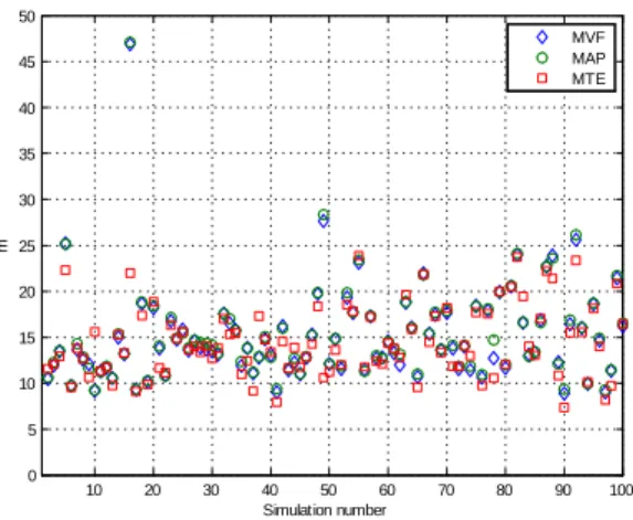
using WSG or MTE using weighted Gaussian Max (WGM) is the exact filter associated to its criterion (they all use approx-imations). We did 100 runs with different noise trajectories. The results are illustrated on figures 4. One may conclude that the MSE of each filter are commensurate, which is not surprising. However, it appears that the MSE of the MTE location filter never exceeds 25 m whereas MAP can have a MSE greater that 45 m (see simulation number 16 and 49). The same phenomena appears for these runs concerning the course estimated. 10 20 30 40 50 60 70 80 90 100 0 5 10 15 20 25 30 35 40 45 50 Simulation number m MVF MAP MTE

Fig. 4. Mean square errors on estimated target location

V. CONCLUSION

In many cases, the outcome of the MTE appears to be an interesting alternative to the minimum variance estimate and can be approximated by Gaussian mixtures in a similar way as for the minimum variance issue. The approximation facilities seem to be similar in both cases. As it is the case for WGS, its implementation leads to the computation of N Kalman filters in parallel (EKFs or UKFs in the nonlinear case). Moreover, this approach allows backward computation of a smoothing trajectory over any past interval under assumption that the past optimal marginal likelihood parameters have been memorized (Gaussian means and variances along with weights).

Note that this approach is particularly interesting when one deals with hybrid systems, it is easy to generalize this approach to such a case. Obviously, there is no sense to compute the mean of symbols. But recall that the marginal conditional pdf p (xtjy0:t) comes from the minimum variance estimator,

the conditional mean. The MTE approach allows to be more coherent avoiding to mix means and Max.

REFERENCES

[1] D. L. Alspach and H. W. Sorenson, “Nonlinear Bayesian estimation using Gaussian sum approximation,” IEEE Transactions on Automatic

Control, vol. 17, no. 4, pp. 439–448, 1972.

[2] N. J. Gordon, D. J. Salmond, and A. F. M. Smith, “Novel approach to Nonlinear/Non-Gaussian Bayesian state estimation,” IEE Proceedings-F, vol. 140, no. 2, pp. 107–113, 1993.

[3] H. A. P. Blom and Y. Bar-Shalom, “The interacting multiple model algorithm for systems with Markovian switching coefficients,” IEEE

Transactions on Automatic Control, vol. 33, no. 8, pp. 780–783, 1988.

[4] R. E. Larson and J. Peschon, “A dynamic programming approach to trajectory estimation,” IEEE Transcations on Automatic Control, vol. 11, no. 3, pp. 537–540, 1966.

[5] H. Cox, “On the estimation of state variable and parameters for noisy dynamic systems,” IEEE Transactions on Automatic Control, vol. 9, no. 4, pp. 376–381, 1964.

[6] A. H. Jazwinski, Stochastic Processes and Filtering Theory, vol. 64. New York and London: Academic Press, 1970.

[7] A. Monin, “Joint maximum likelihood estimation with gaussian mix-ture,” Tech. Rep. 08304, LAAS-CNRS, 2008.

[8] H. W. Sorenson and D. L. Alspach, “Recursive Bayesian estimation using Gaussian sums,” Automatica, vol. 7, pp. 465–479, 1971. [9] K. Turner and F. Fariqi, “A Gaussian sum filtering approach for phase

ambiguity resolution in GPS attitude determination,” IEEE Interational

Conference on Acoustics, Speech and Signal Processing, ICASSP-97,

vol. 5, pp. 4093–4096, 1997.

[10] R. Singer, R. Sea, and K. Housewright, “Derivation and evaluation of improved tracking filters for use in dense multi-target environments,”

IEEE Transactions on Information Theory, vol. 20, no. 4, pp. 423–432,

1974.

[11] D. Reid, “An algorithm for tracking multiple targets,” IEEE Transactions

on Automatic Control, vol. 24, no. 6, pp. 843–854, 1979.

[12] K. Turner and F. Faruqi, “Multiple GPS antenna attitude detremination using Gaussian sum filter,” IEEE TENCON, Digital Signal Processing

Applications, vol. 1, pp. 323–328, 1996.

[13] G. Pulford and S. D.J, “A Gaussian mixture filter for near-far object tracking,” 8th International Conference on Information Fusion, vol. 1, pp. 337–344, 2005.

[14] A. R. Runnalls, “Kullback-leibler approach to gaussian mixture kullback-leibler approach to gaussian mixture kullback-leibler approach to gaussian mixture reduction,” IEEE Transactions on Aerospace and

Electronic Systems, vol. 43, no. 3, pp. 989–999, 2007.

[15] J. L. Williams and P. S. Maybeck, “Cost-function-based gaussian mix-ture reduction for target tracking,” in Proceedings of the 6th

Interna-tional Conference on Information Fusion, vol. 2, pp. 1047–1054, 2003.

[16] M. West, “Approximating posterior distributions by mixtures,” Journal

of the Royal Statistical Society: Series B, vol. 55, no. 409-422, 1993.

[17] I. T. Wing and D. Hatzinakos, “An adaptive Gaussian sum algorithm for RADAR tracking,” IEEE International Conference on Communications, vol. 3, pp. 1351–1355, 1997.

[18] D. Schieferdecker and M. F. Huber, “Gaussian mixture reduction via clustering,” in Proceedings of the 12th International Conference on

Pro-ceedings of the 12th International Conference on Information Fusion,

pp. 1536–1543, 2009.

[19] D. J. Salmond, “Mixture reduction algorithms for target tracking in clutter,” in Proceedings of SPIE Signal and Data Processing of Small

Targets, vol. 1305, pp. 434–445, 1990.

[20] M. Carreira-Perpinñan, “Mode-finding for mixtures of gaussian distribu-tion,” IEEE Transactions on Pattern Analysis and Machine Intelligence, vol. 22, no. 11, pp. 1318–1323, 2000.

[21] E. Wan and R. Van Der Merwe, “The unscented kalman filter for nonlinear estimation,” in Adaptive Systems for Signal Processing,

Com-munications, and Control Symposium 2000. AS-SPCC. The IEEE 2000,