Characterizing K2 Candidate Planetary Systems
Orbiting mass Stars. I. Classifying
Low-mass Host Stars Observed during Campaigns 1–7
The MIT Faculty has made this article openly available.
Please share
how this access benefits you. Your story matters.
Citation
Dressing, Courtney D.; Newton, Elisabeth R.; Schlieder, Joshua E.;
Charbonneau, David; Knutson, Heather A.; Vanderburg, Andrew and
Sinukoff, Evan. “Characterizing K2 Candidate Planetary Systems
Orbiting Low-Mass Stars. I. Classifying Low-Mass Host Stars
Observed During Campaigns 1–7.” The Astrophysical Journal 836,
no. 2 (February 2017): 167 © 2017 The American Astronomical
Society
As Published
http://dx.doi.org/10.3847/1538-4357/836/2/167
Publisher
IOP Publishing
Version
Final published version
Citable link
http://hdl.handle.net/1721.1/109712
Terms of Use
Article is made available in accordance with the publisher's
policy and may be subject to US copyright law. Please refer to the
publisher's site for terms of use.
Characterizing K2 Candidate Planetary Systems Orbiting Low-mass Stars. I. Classifying
Low-mass Host Stars Observed during Campaigns 1
–7
Courtney D. Dressing1,8, Elisabeth R. Newton2,9, Joshua E. Schlieder3,5, David Charbonneau4, Heather A. Knutson1, Andrew Vanderburg4,10, and Evan Sinukoff6,7
1
Division of Geological & Planetary Sciences, California Institute of Technology, Pasadena, CA 91125, USA;dressing@caltech.edu
2
Department of Physics, Massachusetts Institute of Technology, Cambridge, MA 02139, USA
3
IPAC-NExScI, California Institute of Technology, Pasadena, CA 91125, USA
4
Harvard-Smithsonian Center for Astrophysics, Cambridge, MA 02138, USA
5
NASA Goddard Space Flight Center, Greenbelt, MD 20771, USA
6
Institute for Astronomy, University of Hawaí at Mānoa, Honolulu, HI 96822, USA
7
Cahill Center for Astrophysics, California Institute of Technology, 1216 East California Boulevard, Pasadena, CA 91125, USA Received 2016 September 5; revised 2016 November 17; accepted 2016 November 18; published 2017 February 17
Abstract
We present near-infrared spectra for 144candidate planetary systems identified during Campaigns1–7 of the NASA K2 Mission. The goal of the survey was to characterize planets orbiting low-mass stars, but our Infrared Telescope Facility/SpeX and Palomar/TripleSpec spectroscopic observations revealed that 49% of our targets were actually giant stars or hotter dwarfs reddened by interstellar extinction. For the 72stars with spectra consistent with classification as cool dwarfs (spectral types K3–M4), we refined their stellar properties by applying empirical relations based on stars with interferometric radius measurements. Although our revised temperatures are generally consistent with those reported in the Ecliptic Plane Input Catalog (EPIC), our revised stellar radii are typically 0.13R(39%) larger than the EPIC values, which were based on model isochrones that have been shown
to underestimate the radii of cool dwarfs. Our improved stellar characterizations will enable more efficient prioritization of K2 targets for follow-up studies.
Key words: planetary systems– planets and satellites: fundamental parameters – stars: fundamental parameters – stars: late-type – stars: low-mass – techniques: spectroscopic
1. Introduction
Beginning in 2009, the NASA Kepler mission revolutionized exoplanet science by searching for planets transiting roughly 190,000stars and detecting thousands of planet candidates (Borucki et al. 2010, 2011a,2011b; Batalha et al. 2013; Burke et al. 2014). The main Kepler mission ended in 2013 when the second of four reaction wheels failed, thereby destroying the ability of the spacecraft to point stably. Although the two-wheeled Kepler was not able to continue observing the original targets, Ball Aerospace engineers and Kepler team members realized that the torque from solar pressure could be mitigated by selecting fields along the ecliptic plane. In this new mode of operation (known as the K2 Mission), the spacecraft stares at 10,000–30,000 stars per field for roughly 80days before switching to anotherfield along the ecliptic (Howell et al.2014; Van Cleve et al.2016). Unlike in the original Kepler mission, all K2 targets are selected from community-driven Guest Observer (GO) proposals.
The K2 mission design is particularly well-matched for studies of planetary systems orbiting low-mass stars. Although Mdwarfs are intrinsically fainter than Sun-like stars, the prevalence of Mdwarfs within the Galaxy (e.g., Henry et al. 2006; Winters et al. 2015) ensures that there are several thousand reasonably bright low-mass stars per K2field. Due to their smaller sizes and cooler temperatures, these stars are relatively easy targets for planet detection for two main
reasons. First, the transit depth is deeper for a given planet radius. Second, the habitable zones are closer to the stars, thereby increasing both the geometric likelihood that planets within the habitable zone will appear to transit and the number of transits that could be observed during a single K2campaign. For the coolest low-mass stars, the orbital periods of planets within the habitable zone are even short enough that potentially habitable planets would transit multiple times per campaign.
The “Small Star Advantage” of deeper transit depths and higher transit probabilities within the habitable zone is partially offset by the challenge of identifying samples of low-mass stars for observation. When preparing for the original Kepler mission, Brown et al. (2011) conducted an extensive survey of the proposedfield of view to identify advantageous targets and determine rough stellar properties. In contrast, the planning cycle for the K2 mission was too fast-paced to allow for such methodical preparation. During the early days of the K2 mission, the official Ecliptic Plane Input Catalog (EPIC) contained only coordinates, photometry, proper motions, and, when available, parallaxes. Proposers therefore had to use their own knowledge of stellar astrophysics to determine which stars were suitable for their investigations.
More recently, Huber et al. (2016) updated the EPIC to include stellar properties for 138,600 stars. After completing the messy tasks of matching sources from multiple catalogs, converting the photometry to standard systems, and enforcing quality cuts to discard low-quality photometry, Huber et al. (2016) used the Galaxia galactic model (Sharma et al.2011) to generate synthetic realizations of different K2fields. They then determined the most likely parameters for each K2 target star, given the available photometric and kinematic information.
© 2017. The American Astronomical Society. All rights reserved.
8
NASA Sagan Fellow.
9
National Science Foundation Astronomy & Astrophysics Postdoctoral Fellow.
10
When possible, the analysis also incorporated Hipparcos parallaxes (van Leeuwen 2007) and spectroscopic estimates of Teff,log , andg [Fe/H] from RAVE DR4 (Kordopatis et al.
2013), LAMOST DR1 (Luo et al.2015), and APOGEE DR12 (Alam et al.2015).
In all cases, Galaxia used Padova isochrones (Girardi et al. 2000; Marigo & Girardi2007; Marigo et al.2008) to determine
stellar properties. Aware that these isochrones tend to under-predict the radii of low-mass stars(Boyajian et al.2012), Huber et al.(2016) therefore warned that the EPIC radii of low-mass stars may be up to roughly 20% too small. Given that 41% of selected K2 targets are low-mass M and K dwarfs(Huber et al. 2016), improving the radius estimates of low-mass K2 targets is important for maximizing the scientific yield of the K2
Table 1 Observing Conditions
Date Seeing Weather K2
Semester Instru Program (UT) Conditions Targetsa
2015A SpeX 989 2015 Apr 16 0 7–1 0 Clear 2b
SpeX 989 2015 May 5 0 3–0 8 Light wind, clear 5c SpeX 981 2015 Jun 13 0 3–1 0 Cirrus, patchy clouds 2d 2015B SpeX 057, 068 2015 Aug 7 0 5–1 0 Clear at start; closed early due to high humidity 3e SpeX 068 2015 Sep 24 0 5–1 0 Patchy clouds cleared slightly overnight 20
SpeX 072 2015 Oct 14 0 4–1 0 Cirrus 1f
SpeX 068 2015 Nov 26 0 5–2 0 Patchy clouds; high humidity 16
SpeX 068 2015 Nov 27 0 6 Cirrus 16
2016A TSPEC P08 2016 Feb 19 1 2–2 0 Cirrus clouds at start; moderately cloudy by morning 3
SpeX 066 2016 Mar 4 0 5–1 0 Clear 10
SpeX 066 2016 Mar 8 0 5–1 0 Thick, patchy clouds at sunset; thinner clouds by morning 12
SpeX 986 2016 Mar 10 0 9 Cirrus 5g
TSPEC P08 2016 Mar 27 0 9 Clear 15
TSPEC P08 2016 Mar 28 0 9–2 1 Patchy clouds; closed early due to high humidity and fog 9
TSPEC P08 2016 Apr 18 1 1–1 9 Clear 11
SpeX 066 2016 May 5 0 5–1 0 Patchy clouds 11
SpeX 066 2016 May 6 0 3–0 9 Clear 6
SpeX 066 2016 Jun 7 0 4–1 0 Clear 8
2016B SpeX 057 2016 Oct 26 0 5–1 4 Clear 5
Notes.
a
We observed some stars twice on two different nights to assess the repeatability of our analysis.
b
Night awarded to Andrew Howard.
c
Night awarded to Andrew Howard, but observations obtained by Joshua Schlieder.
d
Observations obtained by Evan Sinukoff.
e
Includes one observation acquired by Will Best(Program 057) and two acquired by Courtney Dressing (Program 068).
f
Observations obtained by Kimberly Aller.
g
Night awarded to Andrew Howard, but observations obtained by Courtney Dressing.
Table 2
Targets Observed by theK2 Campaign
Campaign Total Classification in This Paper
Field R.A. Decl. Galactic Targets Cool Hotter
Number (hh:mm:ss) (dd:mm:ss) Latitude(°) Observed Dwarfsa Dwarfs Giants
1 11:35:46 +01:25:02 +59 10 9(90%) 1(10%) 0(0%) 2 16:24:30 −22:26:50 +19 8 0(0%) 4(50%) 4(50%) 3 22:26:40 −11:05:48 −52 12 6(50%) 5(42%) 1(8%) 4 03:56:18 +18:39:38 −26 24 10(42%) 10(42%) 4(17%) 5 08:40:38 +16:49:47 +32 41 27(66%) 13(32%) 1(2%) 6 13:39:28 −11:17:43 +50 34 16(47%) 12(36%) 6(18%) 7 19:11:19 −23:21:36 −15 17 6(35%) 4(24%) 7(41%) 1–7 L L L 146 74(51%) 49(34%) 23(16%) Note. a
Two K2 targets(EPIC 211694226 and EPIC 212773309) have nearby companions that may or may not be physically associated. We classified 74 cool dwarfs in 72 systems.
mission. Both accurate characterization of individual planet candidates and ensemble studies of planetary occurrence demand reliable stellar properties.
Even during the more methodical Kepler era, the properties of low-mass targets were frequently revised. Initially, Brown et al.(2011) characterized all of the targets by comparing multi-band photometry to Castelli & Kurucz (2004) stellar models. This approach worked well for characterizing Sun-like stars, but Brown et al.(2011) cautioned that the Kepler Input Catalog (KIC) temperatures were untrustworthy for stars cooler than 3750K. Batalha et al. (2013) later improved the classifications for many Kepler targets by replacing the original KIC values with parameters of the nearest model star selected from Yonsei-Yale isochrones (Demarque et al. 2004), but those models noticeably underpredict the radii of low-mass stars (Boyajian et al.2012).
Considering the non-planet candidate host stars, Mann et al. (2012) acquired medium-resolution (1150 R 2300) visible spectra of 382putative low-mass dwarf targets. Using those stars as a “training set,” they found that the vast majority (96%±1%) of cool, bright (Kp<14) Kepler target stars were actually giants. For fainter cool stars, giant contamination was much less pronounced (7%±3%). For stars that were correctly classified as dwarfs, Mann et al. (2012) found that the KIC temperatures were systematically 110 K hotter than the values determined by comparing their spectra to the BT-SETTL series of PHOENIX stellar models(Allard et al.2011). In a following paper, Mann et al. (2013b) obtained optical spectra of 123putative low-mass stars hosting 188planet candidates and NIR spectra for a smaller subset of host stars. Flux-calibrating their spectra and comparing them to BT-SETTL stellar models, they derived a set of empirically based relations to determine stellar effective temperatures from spectral indices measured at visible and near-infrared wave-lengths. Mann et al. (2013b) also introduced a set of temperature–radius, temperature–mass, and temperature– luminosity relations based on the sample of stars with well-constrained radii, effective temperatures, and bolometricfluxes. Focusing specifically on the coolest Kepler targets, Muirhead et al.(2012) re-characterized 84cool Kepler Object
of Interest(KOI) host stars by obtaining near-infrared spectra with TripleSpec at the Palomar Hale Telescope. As explained in Rojas-Ayala et al.(2012), they estimated temperatures and metallicities using the H2O-K2 index and the equivalent
widths(EW) of the NaIline at 2.210μm and the CaIline at 2.260μm. Depending on stellar metallicity, the H2O-K2 index
saturates at approximately 3900 K, so this approach cannot be used to characterize mid-K dwarfs. Muirhead et al. (2012) then interpolated the temperatures and metallicities onto Dartmouth isochrones(Dotter et al.2008; Feiden et al.2011) to estimate the radii and masses of their target stars. In a follow-up analysis, Muirhead et al. (2014) expanded their sample to 103cool KOI host stars and updated their mass and radius estimates using newer versions of the Dartmouth isochrones.
Both KOIs and non-KOIs need to be accurately character-ized in order to use the Kepler data to investigate planet occurrence rates, which motivated Dressing & Charbonneau (2013) to refit the KIC photometry using Dartmouth Stellar Evolutionary Models(Dotter et al.2008; Feiden et al.2011) to determine revised properties for 3897 dwarfs cooler than 4000 K. We then used the revised stellar properties to investigate the frequency of planetary systems orbiting low-mass stars.
Recognizing that the stellar parameters inferred in the previous studies were based on stellar models and were therefore likely to underestimate stellar radii, Newton et al. (2015) revised the properties of cool KOI host stars by employing empirical relations based on interferometrically characterized stars. Specifically, Newton et al. (2015) estab-lished relationships between the EWs of Mg and Al features in H-band spectra from Infrared Telescope Facility(IRTF)/SpeX and the temperatures, luminosities, and radii of low-mass stars. Newton et al. (2015) found that the radii of Mdwarf planet candidates were typically 15% larger than previously estimated in the Huber et al. (2014) catalog, which contained a compilation of results from previous studies, including Dressing & Charbonneau (2013), Muirhead et al. (2012, 2014), and Mann et al. (2013b).
Accounting for the systematic effect of previously under-estimated stellar radii, Dressing & Charbonneau (2015) investigated low-mass star planet occurrence in more detail by employing their own pipeline to detect candidates and measure search completeness. Using the full four-year Kepler data set, we found that the mean number of small(0.5 4– RÅ)
planets per late K or early Mdwarf is 2.5±0.2 planets per star for orbital periods shorter than 200days. Within the habitable zone, we estimated occurrence rates of 0.24-+0.08
0.18 Earth-size
planets and 0.21-+0.060.11 super-Earths (1.5 2– RÅ) per star. Those
estimates agree well with rates derived in independent studies (e.g., Gaidos 2013; Gaidos et al. 2014, 2016; Morton & Swift2014).
In order to use the K2 data to conduct similar studies of planet occurrence rates and possibly investigate how the frequency of planetary systems orbiting low-mass stars varies as a function of stellar mass, metallicity, or multiplicity, wefirst need to characterize the stellar sample. In this paper, we classify the subset of K2 target stars that appear to be low-mass stars harboring planetary systems. In the second paper in this series(C. D. Dressing et al. 2017, in preparation), we use our new stellar classifications to revise the properties of the
Figure 1. Magnitude distribution of our full target sample in the Kepler bandpass(Kp; blue) and Ks (red). Our targets have median brightnesses of Ks=10.8 and Kp=13.5. The Kepler bandpass extends from roughly 420 nm to 900 nm with maximum response at 575 nm(Van Cleve & Caldwell2016);
associated planet candidates and identify intriguing systems for follow-up analyses.
In Section 2, we describe our observation procedures and conditions. We then discuss the target sample in Section3and explain our data reduction and stellar characterization proce-dures in Section 4. Finally, we address the implications of our results and conclude in Section 5.
2. Observations
We conducted our observations using the SpeX instrument on the NASA Infrared Telescope Facility (IRTF) over 15partial nights during the 2015A, 2015B, 2016A, and 2016B semesters and the TripleSpec instrument on the Palomar 200″ over fourfull nights during the 2016A semester. Of our IRTF/SpeX nights, 11 were awarded to C.Dressing via programs 2015B068, 2016A066, and 2016B057; the remaining SpeX time was provided by K.Aller, W.Best, A.Howard, and E.Sinukoff. All of our Palomar time was awarded to C.Dressing for program P08.
As detailed in Table1, our observing conditions varied from photometric nights to nights with significant cloud cover through which only our brightest targets were observable. As recommended by Vacca et al. (2003), we removed telluric features from our science spectra using observations of A0V stars acquired under similar observing conditions. Accordingly, we interspersed our science observations with observations of nearby A0V stars. When possible, these A0V stars were within 15° of our target stars and observed within one hour at similar airmasses (difference <0.1 airmasses).
2.1. IRTF/SpeX
For our SpeX observations, we selected the 0 3×15″slit and observed in SXD mode to obtain moderate resolution (R≈2000) spectra (Rayner et al.2003,2004). Due the SpeX upgrade in 2014, our spectra include enhanced wavelength coverage from 0.7 to 2.55μm.
We carried out all of our observations using an ABBA nod pattern with the default settingsof 7 5 separation between positions A and B and 3 75 separation between either pointing and the ends of the slit. For all targets except close binary stars, we aligned the slit with the parallactic angle to minimize systematic effects in our reduced spectra; for binary stars, we rotated the slit so that the sky spectra acquired in the B position would be free of contamination from the second star or so that spectra from both stars could be captured simultaneously. We scaled the exposure times for our targets and repeated the ABBA nod pattern as required so that the resulting spectra would have S/N of 100–200 per resolution element.
We calibrated these spectra by running the standardized IRTF calibration sequence every few hours during our observations and ensuring that each region of the sky had a separate set of calibration frames. The calibration sequence includesflats taken using an internal quartz lamp and wavelength calibration spectra acquired using an internal thorium–argon lamp.
2.2. Palomar/TripleSpec
We acquired our TripleSpec observations using the fixed 1″×30″ slit, which yields simultaneous coverage between 1.0
Table 3
Observations of K2 Targets Classified as Giant Stars
Observation Spectral EPIC Classification EPIC Date Instru Typea Campaign T
eff(K) ep_Teff em_Teff log g(cgs) ep_log g em_log g
202710713 2015 Aug 07 SpeX K4III 2 3817 92 92 0.523 0.168 0.168 203485624 2016 Jun 7 SpeX F2III 2 6237 449 187 3.848 0.228 0.020 203776696 2016 Mar 27 TSPEC F8III 2 6113 1219 508 4.143 0.270 0.315 205064326 2016 Jun 7 SpeX K0III 2 4734 75 75 2.946 0.144 0.144 206049452 2015 Sep 24 SpeX M2III 3 4553 191 109 4.671 0.035 0.042 210769880 2015 Sep 24 SpeX K2III 4 4018 118 802 4.809 2.400 0.060 210843708 2015 Sep 24 SpeX K3III 4 4823 120 90 2.456 0.075 0.450 211098117 2015 Sep 24 SpeX K0III 4 3858 186 186 4.870 0.070 0.084 211106187 2015 Nov 27 SpeX G5III 4 5321 96 192 4.561 0.164 0.020 211351816 2015 Nov 27 SpeX K2III 5 4742 96 76 2.984 0.483 0.345 212311834 2016 Apr 18 TSPEC M1III 6 5199 156 188 3.631 0.890 0.890 212443457 2016 Mar 8 SpeX K0III 6 4804 144 173 4.598 0.025 0.030 212443457 2016 Jun 7 SpeX K0III 6 4804 144 173 4.598 0.025 0.030 212473154 2016 Jun 7 SpeX K0III 6 4570 136 136 2.365 0.682 0.186 212586030 2016 Mar 8 SpeX K1III 6 4814 76 76 3.328 0.144 0.144 212644491 2016 Apr 18 TSPEC K1III 6 4940 96 96 2.505 0.306 0.663 212786391 2016 Mar 27 TSPEC G5III 6 4688 109 73 2.164 0.912 0.570 214629283 2016 May 5 SpeX M3III 7 3508 150 150 0.241 0.310 0.558 214799621 2016 May 5 SpeX K4III 7 4375 132 132 2.184 0.360 0.216 215030652 2016 Jun 7 SpeX M0III 7 3935 79 79 0.778 0.250 0.300 215090200 2016 May 5 SpeX K0III 7 4596 115 172 2.422 0.145 0.203 215174656 2016 May 6 SpeX K7III 7 3814 92 115 0.538 0.150 0.150 215346008 2016 Jun 7 SpeX K4III 7 4038 165 132 1.357 1.216 0.228 218006248 2016 May 5 SpeX M2III 7 3330 33 33 0.088 0.070 0.182
Note.
a
Spectral types are coarse assignments based on visual inspection of the near-infrared spectra collected in this paper. The assigned spectral types have errors of roughly±1 subtype. (See Section4.1for details.)
and 2.4μm at a spectral resolution of 2500–2700 (Herter et al. 2008). In order to decrease the effect of bad pixels on the detector, we adopted the four-position ABCD nod pattern used
by Muirhead et al.(2014) rather than the two-position ABBA pattern we used for our SpeX observations. With the exception of double star systems for which we altered the slit rotation to
Table 4
Observations of K2 Targets Classified as Hotter Dwarfs
Observation
Spectral EPIC Classification
EPIC Date Instru Typea Campaign Teff(K) ep_Teff em_Teff log g(cgs) ep_log g em_log g
201754305 2015 Jun 13 SpeX K3Vb 1 4755 113 113 4.642 0.045 0.045 204890128 2016 Mar 27 TSPEC K2V 2 5213 188 707 3.848 0.535 0.535 205084841 2016 Mar 27 TSPEC K0V 2 4793 207 207 2.369 0.205 0.656 205145448 2016 Jun 7 SpeX G5V 2 5700 390 57 3.841 1.362 0.020 205145448 2016 May 5 SpeX G5V 2 5700 390 57 3.841 1.362 0.020 205686202 2016 May 5 SpeX K1V 2 3809 68 1432 4.889 0.399 0.084 206055981 2016 Oct 26 SpeX K3Vb 3 4522 45 73 4.668 0.028 0.024 206055981 2015 Nov 26 SpeX K3Vb 3 4522 45 73 4.668 0.028 0.024 206056433 2016 Oct 26 SpeX K4Vb 3 4506 109 54 4.666 0.025 0.045 206056433 2015 Nov 26 SpeX K4Vb 3 4506 109 54 4.666 0.025 0.045 206096602 2015 Aug 07 SpeX K3Vb 3 4617 138 138 4.649 0.030 0.036 206096602 2015 Sep 24 SpeX K3Vb 3 4617 138 138 4.649 0.030 0.036 206135267 2015 Sep 24 SpeX K2V 3 5165 123 215 3.678 0.286 0.130 206144956 2015 Sep 24 SpeX K2V 3 4848 78 97 4.611 0.025 0.025 210414957c 2015 Nov 26 SpeX G2V 4 5404 107 86 3.779 0.196 0.020 210423938 2015 Nov 27 SpeX K3Vb 4 4856 114 171 2.876 0.582 0.485 210577548 2015 Nov 26 SpeX K2V 4 L L L L L L 210609658 2015 Sep 24 SpeX K2V 4 4963 97 97 3.268 0.416 0.260 210731500 2015 Nov 27 SpeX K1V 4 5406 168 168 4.472 0.476 0.068 210754505 2015 Nov 26 SpeX G5V 4 6041 120 120 4.224 0.168 0.140 210793570 2015 Nov 26 SpeX K3Vb 4 4896 118 118 3.242 0.609 0.435 210852232 2015 Nov 27 SpeX K0V 4 5437 167 301 4.527 0.384 0.040 211058748 2015 Nov 27 SpeX K2V 4 5070 81 243 4.615 0.060 0.110 211133138 2015 Nov 26 SpeX K2V 4 5742 367 275 3.965 0.150 0.500 211418290 2015 Nov 27 SpeX G5V 5 5182 126 126 2.461 0.055 1.111 211529065 2016 Mar 28 TSPEC K4Vb 5 4742 167 167 4.621 0.036 0.030 211579683 2016 Mar 28 TSPEC K3Vb 5 4829 57 76 3.432 1.045 1.254 211619879 2016 Mar 4 SpeX K3Vb 5 4403 303 216 4.706 0.045 0.081 211779390 2015 Nov 26 SpeX K3Vb 5 4472 122 87 4.705 0.065 0.195 211783206 2016 Mar 28 TSPEC K5Vb 5 4855 94 94 3.324 0.655 1.310 211796070 2016 Mar 4 SpeX K3Vb 5 4564 91 91 4.665 0.025 0.035 211797637 2016 Mar 27 TSPEC K5Vb 5 4521 108 135 4.696 0.055 0.121 211913977 2015 Nov 27 SpeX K3Vb 5 4825 58 77 4.607 0.025 0.040 211970147 2016 Mar 8 SpeX K3Vb 5 4576 54 72 4.667 0.035 0.025 212012119 2015 Nov 27 SpeX K3Vb 5 4837 78 58 3.178 0.715 0.325 212132195 2015 Nov 27 SpeX K3Vb 5 4631 75 112 4.656 0.036 0.020 212138198 2015 Nov 27 SpeX K3Vb 5 4975 99 139 4.577 1.218 0.030 212315941 2016 Mar 28 TSPEC K3Vb 6 4909 78 118 4.628 0.025 0.040 212470904 2016 Mar 8 SpeX K5Vb 6 4761 97 97 4.617 0.042 0.030 212521166d 2016 Mar 10 SpeX K2V 6 4841 145 174 4.628 0.030 0.025 212525174 2016 Mar 27 TSPEC K4Vb 6 4163 41 100 4.876 0.084 0.020 212530118 2016 Mar 4 SpeX K5Vb 6 4175 41 49 4.824 0.045 0.108 212532636 2016 Mar 28 TSPEC K3Vb 6 4519 109 73 4.698 0.030 0.042 212572439 2016 Mar 10 SpeX K2V 6 4972 59 49 4.593 0.020 0.039 212572439 2016 Mar 27 TSPEC K2V 6 4972 59 49 4.593 0.020 0.039 212730483 2016 Mar 4 SpeX K3Vb 6 4612 55 55 4.657 0.040 0.020 212737443 2016 Mar 28 TSPEC K3Vb 6 4542 298 149 4.708 0.040 0.088 212756297 2016 Mar 10 SpeX K5Vb 6 4429 78 131 4.729 0.078 0.104 212757039 2016 Apr 18 TSPEC K1V 6 5510 223 223 4.574 0.088 0.066 212779596 2016 Jun 7 SpeX K5Vb 6 4731 77 77 4.623 0.036 0.036 212779596 2016 Mar 8 SpeX K5Vb 6 4731 77 77 4.623 0.036 0.036 214173069 2016 Oct 26 SpeX K3Vb 7 4659 150 75 4.633 0.035 0.025 214173069 2016 May 6 SpeX K3Vb 7 4659 150 75 4.633 0.035 0.025 216111905 2016 May 6 SpeX G8V 7 5221 126 84 4.543 0.760 0.040 217192839 2016 May 6 SpeX K2V 7 4563 89 107 4.682 0.042 0.133 219114906 2016 May 6 SpeX K2V 7 4523 108 90 4.662 0.030 0.042 Notes. a
Spectral types are coarse assignments based on visual inspection of the near-infrared spectra collected in this paper. The assigned spectral types have errors of roughly±1 subtype. (See Section4.1for details.)
b
In general, we list stars with spectral types of K3V or later in the cool dwarf sample rather than the hotter dwarf sample. However, these stars had estimated temperatures>4800 K or estimated radii >0.8R , which are beyond the validity range of the Newton et al. (2015) relations.
cPossible fainter nearby star identified in the Gemini AO image acquired by D.Ciardi (https://exofop.ipac.caltech.edu/k2/edit_target.php?id=210414957). d
place both stars in the slit when possible, we left the slit in a fixed east–west orientation. We calibrated our spectra using dome darks and domeflats acquired at both the beginning and end of the night.
3. Target Sample
The objective of our observing campaign was to determine the properties of K2 target stars and assess the planethood of associated planet candidates. Consequently, our targets were selected from lists of K2 planet candidates compiled by A.Vanderburg and the K2 California Consortium (K2C2). These early target lists are preliminary versions of planet candidate catalogs such as those published in Vanderburg et al. (2016) and Crossfield et al. (2016).
Of the 144K2 targets observed, 99 (69%) appear in unpublished lists provided by A. Vanderburg, 28 (19%) were published in the Vanderburg et al. (2016) catalog, and 77 (53%) were reported in previously unpublished lists generated by K2C2.(These totals sum to >100% due to partial overlap between the Vanderburg and K2C2 candidate lists.) The K2C2
planet candidates from K2 Campaigns 0–4 were later published in Crossfield et al. (2016). Although we did not consult these catalogs for initial target selection, our target sample also contains 46systems from Barros et al. (2016), 26stars from Pope et al.(2016), 5stars from Foreman-Mackey et al. (2015), 5stars from Montet et al. (2015), and 4stars from Adams et al.(2016).
The Vanderburg and K2C2 catalogs contain all of the planet candidates detected by the corresponding pipeline(K2SFF and TERRA, respectively) in the K2 light curves of stars proposed as individual GO targets. Neither pipeline considers stars observed as part of “super-stamps.” Due to the heterogenous nature of the K2 target lists and the limited information provided in the EPIC during early K2 campaigns, the selected target sample is heavily biased. As noted by Huber et al. (2016), the K2 target lists are biased toward cool dwarfs. Overall, the set of stars observed during Campaigns1–8 consisted primarily of K and M dwarfs(41%), F and G dwarfs (36%), and Kgiants (21%), but the giant fraction was higher forfields close to the galactic plane (see Table2) than for fields at higher galactic latitude(Huber et al.2016). Many GOs used a magnitude cut when proposing targets, which may have increased the representation of multiple star systems within the selected sample.
Due to the design of the K2 mission, our K2 targets were concentrated in distinctfields of the sky each spanning roughly 100 square degrees. We note the number of targets observed from each campaign in Table 2. As shown in Figure 1, the magnitude distribution of our K2 targets ranged from 6.2 to 13.1 in Ks, with a median Ks magnitude of 10.8. In the Kepler bandpass (similar to V-band), our targets had brightnesses of Kp=9.0–16.3 and a median brightness of Kp=13.5.
With each K2 data release, we initially prioritized observations of stars harboring small planet candidates
Figure 2.Distribution of visually assigned spectral types for the 74stars in our cool dwarf sample.
Figure 3.Repeatability of our equivalent width measurements when using the same instrument for both observations (magenta points) or different instruments for each observation (navy points). The 75 data points plotted here are the EW measured forfive Mg and Al features in 30 spectra of 15 candidate low-mass dwarfs(two observations per star). Eight stars were later classified as cool dwarfs (large circles; spectral types K7, M0, and M1) and seven were classified as hotter dwarfs (small points). For reference, the gray dashed line marks zero difference between the two EW measurements.
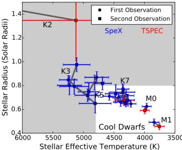
Figure 4.Repeatability of parameter estimates for the subsample of 15 stars with two observations. The data points mark the estimated temperatures and radii found by applying the Newton et al.(2015) EW relations to the first
observations (circles) and second observations (squares) of each star. The colors differentiate between observations made using SpeX on the IRTF(blue) and TSPEC on the Palomar 200″ (red). The thick gray lines connect the two classifications for each star. The cluster of points near 4350 K and 0.7R
contains five K7 dwarfs observed twice each. The white box indicates the boundaries of our cool dwarf sample:Teff<4800K,R<0.8R.
(estimated planet radius <4RÅ) and systems that could
potentially be well-suited for high-precision radial velocity observations (host star brighter than V=12.5 and estimated radial velocity semi-amplitude K>2 m s−1). Once we had exhaustedthose targets, we worked down the target list and observed increasingly fainter host stars harboring larger planets. Our goal was to select late K dwarfs and M dwarfs, but the initial stellar classifications were uncertain, particu-larly for thefirst K2 fields when the Huber et al. (2016) EPIC stellar catalog was not yet available. To ensure that few low-mass stars were excluded from our analysis, we adopted lenient criteria when selecting potential target stars. Our rough guidelines were J−K>0.5 and, for stars with coarse initial temperature estimates, temperatures cooler than 4900 K. Concentrating on the brightest targets biased our sample toward giant stars and binary stars. Similarly, our selected J−K color-cut also boosted the giant fraction by excluding hotter dwarfs with bluer J−K colors without discarding giant stars with extremely red J−K colors. The binary boost due to prioritizing bright targets may have been partially
offset by our avoidance of stars with nearby companions detected in follow-up adaptive optics images.
4. Data Analysis and Stellar Characterization We performed initial data reduction using the publicly available Spextool pipeline (Cushing et al. 2004) and a version customized for use with TripleSpec data (available upon request from M. Cushing). Both versions of the pipeline include the xtellcor telluric correction package (Vacca et al.2003). As recommended in the Spextool manual, we selected the Paschen δ line at 1.005 μm when generating the convolution kernel used to apply the observed instrumental profile and rotational broadening to the Vega model spectrum.
4.1. Initial Classification
After completing the Spextool reduction, we used an interactive Python-based plotting interface to compare our spectra to the spectra of standard stars from the IRTF Spectral Library(Rayner et al.2009). We allowed each model spectrum to shift slightly in wavelength space to accommodate differences in stellar radial velocities. Considering the J, H, and K bandpasses independently, we assessed the c2of afit of
each model spectrum to our data and recorded the dwarf and giant models with the lowestχ2.
We then considered the target spectrum holistically and assigned a single classification to the star. Although the focus of this analysis was to characterize planetary systems orbiting low-mass dwarfs, our target sample did include contamination from hotter and evolved stars. We list the 23giants and 49hotter dwarfs in Tables3 and 4, respectively. We did not include either group in the more detailed analyses described in Section4.2. For the purposes of identifying contamination, we rejected all stars that we visually classified as giants or dwarfs with spectral types earlier than K3. Table 4 also includes all stars for which the Newton et al. (2015) routines yielded estimated temperatures above 4800 K or radii larger than 0.8
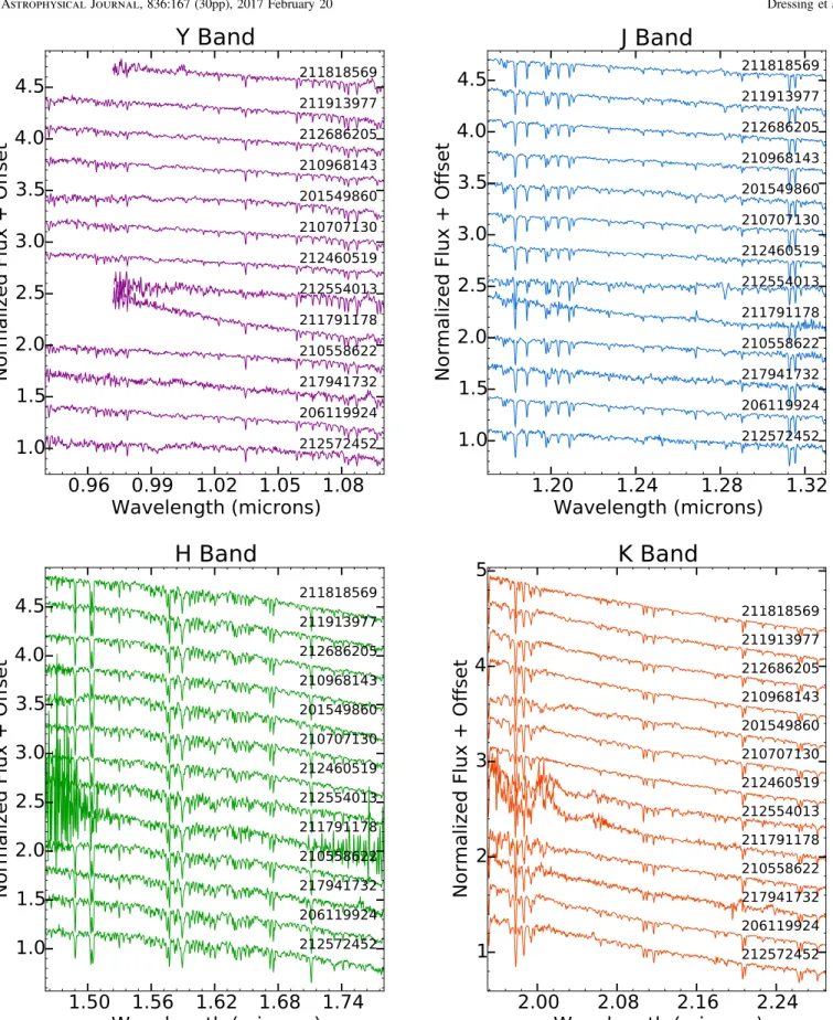
R (see Section 4.2). We display the reduced spectra for all targets in theAppendix. We have also posted our spectra and stellar classifications on the ExoFOP-K2 follow-up website.11
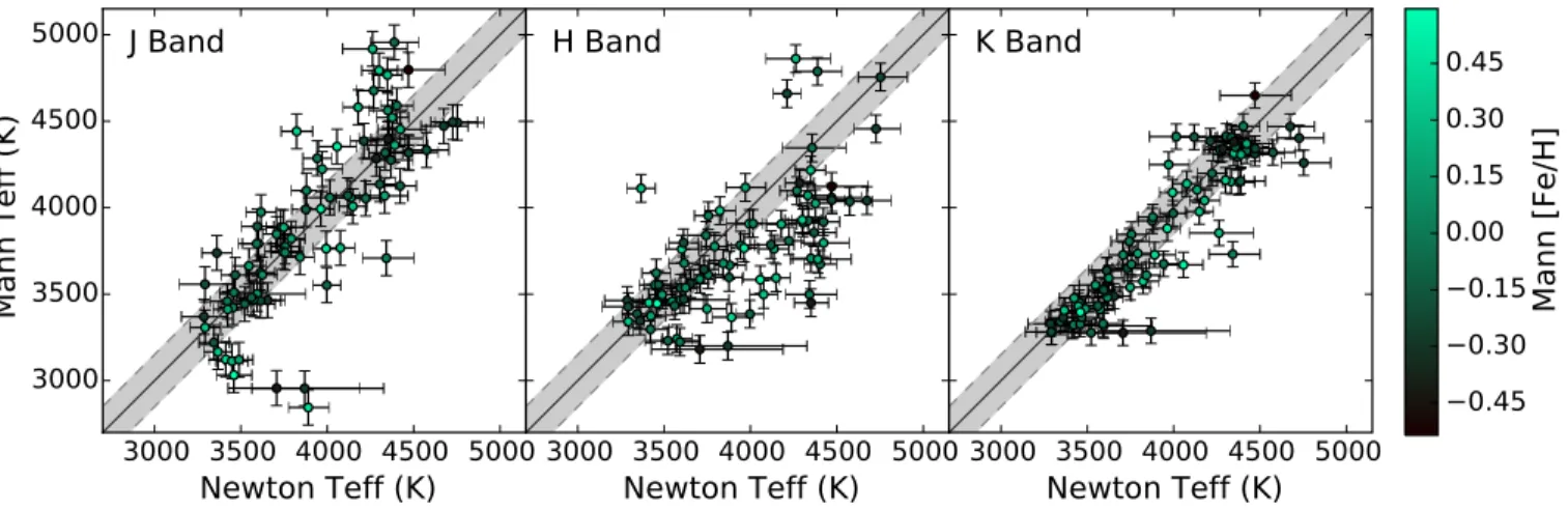
Figure 5.Comparison of temperatures derived using EW-based estimates from Newton et al.(2015) and spectral indices from Mann et al. (2013b) in Jband (left),
Hband (middle), and Kband (right). Points within the shaded region lie within 150 K of a one-to-one relation (solid line). All points are color-coded by [Fe/H], as indicated by the colorbar.
Figure 6.Numerical spectral types automatically derived from the H O2 -K2
index vs. our visually determined spectral types. The points are color-coded based on the EW-based temperature estimate resulting from the Newton et al. (2015) relations. The gray shaded region denotes spectral types that fall within
one spectral type of a one-to-one relation. For reference, the rainbow shading also denotes the spectral type ranges. We assigned visual spectral types at integer values, but the points are horizontally offset for clarity.
11
Figure2displays the spectral type distribution of the stars in the selected cool dwarf sample. The sample includes stars with spectral types between K3 and M4, with a median spectral type of M0. These spectral types are rather coarse visual assign-ments(±1 subclass), so the spike at M3V may be a quirk of the particular template stars used for spectral type assignment rather than a true feature of the distribution. Due to the small sample size, the spike can also be explained by Poisson counting errors.
4.2. Detailed Stellar Characterization
For the stars that were visually identified as dwarfs with spectral types of K3 or later, we used a series of empirical relations to refine the stellar classification. We began by using the publicly available, IDL-based tellrv12 and nirew13
packages developed by Newton et al. (2014, 2015) to shift each spectrum to the stellar rest frame on an order-by-order basis, measure the equivalent widths of key spectral features, and estimate stellar properties. Specifically, the packages employ empirically based relations linking the equivalent widths of H-band Al and Mg features to stellar temperatures, radii, and luminosities(Newton et al.2015). These relations are appropriate for stars with spectral types between mid-K and mid-M (i.e., temperatures of 3200–4800 K, radii of0.18 <R<0.8R, and
luminosities of -2.5<logL L< -0.5). The relations were
calibrated using IRTF/SpeX spectra (Newton et al.2015) so we downgraded the Palomar/TSPEC spectra to match the lower resolution of IRTF/SpeX data before applying the relations. We note that neglecting the change in resolution can lead to systematic 0.1 Å differences in the measured EW due to variations in the amount of contamination included in the designated wavelength interval(Newton et al.2015). As shown in Figure 3, we find generally consistent equivalent widths in spectra acquired on different occasions even if the two observations used separate instruments under variable observing conditions. Specifically, the median absolute difference in equivalent widths for the five cool dwarfs with repeated measurements using the same instrument was 0.2 Å(0.9σ). The median absolute difference for the three cool dwarfs with measurements from different instruments was 0.3 Å(1.9σ).
In the original formulation of the measure_hband stellar characterization routine, the errors on stellar parameters are determined via a Monte Carlo simulation in which multiple realizations of noise are added to the spectra and the equivalent widths of features are re-measured. The errors are then determined by combining the random errors in the resulting EWs with the intrinsic scatter in the relations. This approach yields useful errors, but the adopted stellar parameters are taken from a single realization of the noise. For high SNR spectra, variations in the simulated noise might not lead to large changes in stellar properties, but for lower SNR spectra the estimated properties can differ considerably from one realization to the next. Several of our spectra have SNR of less than 200, which was the threshold used in the Newton et al.(2015) study. Accordingly, we altered measure_hband to calculate the temperatures, luminosities, and radii for each realization of the noise and report the 50th, 16th, and 84th percentiles as the best-fit values, lower error bars, and upper error bars, respectively.
Our changes significantly improve the reproducibility of temperature, luminosity, and radius estimates for stars with lower SNR spectra. For example, we repeated the classification of the M2dwarf EPIC206209135 five times using both the original and modified versions of measure_hband. For each classification, we determined parameter errors by generating 1000noise realizations. The original code yielded estimated temperatures ranging from 3267 to 3461 K, radii of 0.32–0.35
R , and -1.94logL L-1.85. The variations in the
assigned temperatures and luminosities of 194K and
L
0.09 log were significantly larger than the individual error estimates of 85K and0.06 logL and the spread in assigned
radii of 0.03R was equal to the individual radius errors. In
comparison, our new method found Teff=336087 K,
=
R 0.33 0.03R , and logL = -1.870.06 logL in
all cases. Due to the asymmetry of the resulting temperature and radius distributions for some stars, we also report separate upper and lower error bounds instead of forcing the errors to be symmetric in all cases. (EPIC 2106209135 is an example of a star with naturally symmetric errors.)
We confirmed that our cool dwarf classifications were repeatable by comparing our parameter estimates for the 15 stars observed on two different observing runs. Figure4reveals satisfactory agreement in the temperature and radius estimates for the eight stars cooler than 4800 K, the designated upper limit for our cool dwarf sample. Our results for the seven hotter
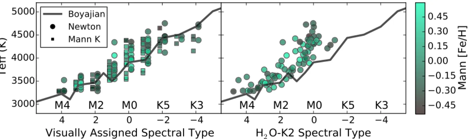
Figure 7.Temperatures from Newton et al.(2015) EW-based relation (circles) and Mann et al. (2013b) K-band relation (squares) vs. visually assigned spectral type
(left) and automatically assigned H O2 -K2 index-based spectral types(right). For reference, the black line shows the spectral types and temperatures reported by
Boyajian et al.(2012) for interferometrically characterized stars. Note that Boyajian et al. (2012) report temperatures at half spectral types between M0 and M4. All
points are color-coded by[Fe/H] as indicated by the colorbar.
12https://github.com/ernewton/tellrv 13
Table 5
Observation Dates, Spectral Types, and Radial Velocities for Stars Classified as Cool Dwarfs
Observation Spectral H2O-K2 RVd EPIC Campaign Date Instru Typea Indexb SpTypec (km s−1)
201205469 1 2015 Jun 13 SpeX K7V 1.03 0.39 −4.0 201208431 1 2015 May 05 SpeX K7V 1.04 0.17 16.4 201345483 1 2015 May 05 SpeX M0V 1.03 0.49 4.5 201549860 1 2015 Nov 26 SpeX K4V 1.03 0.49 54.7 201617985 1 2015 Apr 16 SpeX M1V 1.01 0.93 4.4 201635569 1 2015 May 05 SpeX M0V 1.02 0.67 6.6 201637175 1 2015 May 05 SpeX K7V 1.01 1.02 −8.4 201717274 1 2015 May 05 SpeX M2V 0.89 3.93 43.1 201855371 1 2015 Apr 16 SpeX K5V 1.02 0.65 −11.9 205924614 3 2015 Sep 24 SpeX K7V 1.00 1.24 0.9 205924614 3 2015 Nov 26 SpeX K7V 1.02 0.78 4.4 206011691 3 2015 Aug 07 SpeX K7V 1.04 0.14 9.5 206011691 3 2015 Sep 24 SpeX K7V 1.04 0.31 4.2 206119924 3 2015 Sep 24 SpeX K7V 1.04 0.20 −16.8 206209135 3 2015 Sep 24 SpeX M2V 0.91 3.46 −38.1 206312951 3 2015 Sep 24 SpeX M1V 0.98 1.64 −14.0 206318379 3 2015 Sep 24 SpeX M4V 0.88 4.07 11.7 210448987 4 2015 Nov 27 SpeX K3V 1.04 0.13 −15.9 210489231 4 2015 Sep 24 SpeX M1V 0.98 1.75 −56.6 210508766 4 2015 Sep 24 SpeX M1V 1.02 0.75 −0.4 210558622 4 2015 Oct 14 SpeX K7V 1.03 0.47 −0.1 210558622 4 2015 Nov 26 SpeX K7V 1.03 0.36 −2.6 210564155 4 2015 Nov 27 SpeX M2V 0.91 3.46 36.5 210707130 4 2015 Sep 24 SpeX K5V 1.03 0.42 −2.4 210750726 4 2015 Sep 24 SpeX M1V 0.94 2.59 2.5 210838726 4 2015 Sep 24 SpeX M1V 0.99 1.39 18.6 210968143 4 2015 Sep 24 SpeX K5V 1.04 0.31 20.9 211077024 4 2015 Nov 26 SpeX M3V 0.92 3.19 23.2 211305568 5 2015 Nov 27 SpeX M1V 0.99 1.50 29.7 211331236 5 2015 Nov 26 SpeX M1V 0.99 1.48 2.0 211331236 5 2016 Apr 18 TSPEC M1V 0.96 2.24 −5.3 211336288 5 2016 Mar 27 TSPEC M0V 1.03 0.55 19.4 211357309 5 2015 Nov 27 SpeX M1V 0.99 1.38 18.5 211428897e 5 2015 Nov 26 SpeX M2V 0.95 2.52 25.6 211509553 5 2016 Mar 27 TSPEC M0V 0.97 1.87 −14.7 211680698 5 2016 Mar 28 TSPEC K3V 1.02 0.60 −29.4
211694226A 5 2016 Mar 8 SpeX M3V 0.93 2.98 21.2
211694226B 5 2016 Mar 8 SpeX M3V 0.93 2.84 24.0 211762841 5 2016 Mar 4 SpeX K7V 1.03 0.47 24.6 211770795 5 2016 Apr 18 TSPEC K5V 1.04 0.17 −44.3 211791178 5 2016 Mar 27 TSPEC M0V 1.01 0.96 61.5 211799258 5 2016 Mar 8 SpeX M3V 0.93 2.78 44.6 211817229 5 2016 Mar 4 SpeX M4V 0.85 4.91 28.2 211818569 5 2016 Feb 19 TSPEC K5V 1.06 −0.16 24.9 211822797 5 2016 Mar 27 TSPEC K7V 1.00 1.23 28.3 211826814 5 2016 Feb 19 TSPEC M4V 0.90 3.72 24.1 211831378 5 2016 Apr 18 TSPEC M0V 0.92 3.08 3.7 211839798 5 2016 Mar 4 SpeX M4V 0.86 4.62 30.5 211924657 5 2016 Mar 8 SpeX M3V 0.89 3.87 40.0 211965883 5 2016 Mar 27 TSPEC M0V 1.08 −0.68 37.3 211969807 5 2016 Mar 8 SpeX M1V 0.98 1.78 33.5 211970234 5 2016 Apr 18 TSPEC M4V 0.87 4.35 −8.5 211988320 5 2016 Mar 27 TSPEC K7V 1.09 −0.86 79.1 212006344 5 2015 Nov 26 SpeX M0V 1.02 0.65 −13.3 212006344 5 2016 Feb 19 TSPEC M0V 1.01 0.97 −15.5 212069861 5 2015 Nov 26 SpeX M0V 1.02 0.76 25.3 212154564 5 2016 Mar 27 TSPEC M3V 0.95 2.46 20.9 212354731 6 2016 Mar 28 TSPEC M3V 0.88 4.12 −24.4 212398486 6 2016 Mar 4 SpeX M2V 0.93 2.89 −19.0 212443973 6 2016 Mar 27 TSPEC M3V 0.96 2.05 0.7 212460519 6 2016 Mar 8 SpeX K7V 1.05 0.09 −1.6 212554013 6 2016 Apr 18 TSPEC K3V 1.10 −1.12 −60.0
stars are less consistent, but the relations from Newton et al. (2015) are not valid at those temperatures.
4.2.1. Stellar Effective Temperature
For comparison, we also determined stellar effective temperatures using the J-, H-, and K-band temperature-sensitive indices and relations presented by Mann et al. (2013b). We then applied the temperature–metallicity–radius relation from Mann et al.(2015) to assign stellar radii. Next, we determined luminosities and masses from the estimated stellar effective temperatures using relations 7 and 8 from Mann et al. (2013b). These relations are based on stars with effective temperatures between 3238 and 4777 K and radii between 0.19 and 0.78R.
In Figure 5, we plot the temperature estimates generated using the Newton et al.(2015) pipeline against those from the Mann et al. (2013b) relations. The Mann H-band-based temperatures display considerable scatter and are system-atically lower than the three other estimates (the temperatures based on the Newton et al. (2015) routines, the J-band temperatures, and the K-band temperatures). This discrepancy, which is most noticeable for stars hotter than 4000 K, is likely caused by saturation of the index as the continuumflattens for hotter stars. The J-band temperatures also display large scatter,
but they are more centered along a one-to-one relation than the H-band estimates. Due to the much tighter correlation observed between the K-band temperatures and the EW-based temper-ature estimates, we adopt the K-band tempertemper-atures as the “Mann temperatures” for our stars. We also see discrepancies for stars withTeff<3500. There are three stars for which the temperature inferred using the Newton et al.(2015) relations is larger than that inferred from the J-, H-, and K-band temperatures, The error bars in the temperature inferred from the Newton et al.(2015) relations are also large. This is caused by the disappearance of the Mg and Al features in the coolest dwarf stars, which tends to result in an overestimate of Teff. Al
is weaker at lower metallicity, consistent with this effect only being seen in metal-poor stars at the limits of the calibration.
Newton et al.(2015) also compared temperature estimates derived using their empirical relations with those based on the Mann et al. (2013b) temperature-sensitive indices. They found large standard deviations of sDT=140K and
sDT =170K in Jband and Hband, respectively, between temperatures determined using each method, which they attributed to telluric contamination. In contrast, the standard deviation between the Newton et al.(2015) estimates and the Mann et al.(2013b) K-band estimates was only s =DT 90 K,
suggesting that the K-band relation is less contaminated by telluric features.
Table 5 (Continued)
Observation Spectral H2O-K2 RVd EPIC Campaign Date Instru Typea Indexb SpTypec (km s−1)
212565386 6 2016 Mar 10 SpeX M1V 0.97 1.98 −38.7 212572452 6 2016 Mar 10 SpeX K7V 1.06 −0.17 5.7 212572452 6 2016 Mar 27 TSPEC K7V 1.05 −0.03 6.0 212628098 6 2016 Apr 18 TSPEC K7V 0.96 2.05 −2.2 212634172 6 2016 Mar 4 SpeX M3V 0.93 2.95 23.2 212679181 6 2016 Mar 4 SpeX M3V 0.95 2.45 13.3 212679798 6 2016 Apr 18 TSPEC M0V 0.96 2.06 4.0 212686205 6 2016 Mar 8 SpeX K4V 1.04 0.14 −9.6 212690867 6 2016 Mar 8 SpeX M2V 0.95 2.30 6.5 212773272 6 2016 Apr 18 TSPEC M3V 0.95 2.51 −7.2 212773309 6 2016 Mar 28 TSPEC M0V 1.01 0.94 −13.6 212773309B 6 2016 Mar 28 TSPEC M3V 0.92 3.03 −4.1 213951550 7 2016 May 6 SpeX M3V 0.93 2.81 −77.2 214254518 7 2016 May 5 SpeX K7V 1.05 0.09 17.6 214254518 7 2016 Oct 26 SpeX K7V 1.04 0.22 17.3 214522613 7 2016 May 5 SpeX M1V 0.96 2.20 35.9 214787262 7 2016 May 5 SpeX M3V 0.91 3.27 −24.1 216892056 7 2016 May 5 SpeX M2V 0.94 2.69 −82.8 217941732 7 2016 May 5 SpeX K5V 1.03 0.41 −49.8 217941732 7 2016 Oct 26 SpeX K5V 1.03 0.40 −50.9 Notes. a
Spectral types are coarse assignments based on visual inspection of the near-infrared spectra collected in this paper. The assigned spectral types have errors of roughly±1 subtype. (See Section4.1for details.)
b
H2O-K2 index(Rojas-Ayala et al.2012). Although we report H O2 -K2 indices and index-based spectral types for the full cool dwarf sample, these values are
meaningless for the hotter stars.
c
Spectral type estimated using the H O2 -K2—spectral type relation introduced by Newton et al. (2014). On this scale, a spectral type of 0 corresponds to MV0 and
positive values indicate correspondingly later M dwarf spectral types(e.g., 2=M2V). Negative values indicate K subtypes (i.e., −1=K7V, −2=K5V).
d
Reported absolute radial velocities are the median of the values estimated by cross-correlating the telluric lines in our J-, H-, and K-band spectra with a theoretical atmospheric transmission spectrum using the tellrv framework developed by Newton et al. (2014).
e
Keck AO imaging by D.Ciardi and Gemini speckle imaging by M.Everett revealed that the star is actually a visual binary with a separation of roughly 1 1(https:// exofop.ipac.caltech.edu/k2/edit_target.php?id=211428897).
For our sample of stars, the agreement between the two methods is much worse: we measure standard deviations of 278, 311, and 162K for the temperature differences between the EW-based estimates and the estimates based on the J-band,
H-band, and K-band spectral indices, respectively. The median temperature differences are 13, 143, and 64K for Jband, Hband, and Kband, respectively, with the EW-based estimates higher than the spectral index-based estimate for
Figure 8.Estimated metallicities for the 63 cool dwarfs with spectral types of K7 or later. The top two panels display the distribution of[Fe/H] (left) and [M/H] (right) calculated using separate relations from Mann et al. (2013a) for H-band (blue) and K-band (green) spectra. The bottom two panels display the distributions of
differences in the H-band and K-band estimates of[M/H] (left) and [Fe/H] (right). The green lines indicate the median values (solid lines) and the 16th and 84th percentile values(dashed lines).
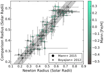
Figure 9.Comparison of radii derived directly using the Newton et al.(2015)
relations and indirectly via the Mann et al. (2015, circles) temperature– metallicity–radius relation or Boyajian et al. (2012, squares) temperature– radius relation. Points within the shaded region lie within 0.05R of a one-to-
one relation(solid line). The data points are color-coded by [M/H] as measured using relations from Mann et al.(2013a).
Figure 10.Comparison of temperatures and radii derived using relations from Newton et al.(2015) and Mann et al. (2015). The gray lines connect the values
from the Newton relations(blue circles) and Mann relation (green squares) for each star. The three mid-M dwarfs highlighted with light blue circles have Al-a EW below the calibration range for the Newton temperature relations. For those three stars only, we adopt the Mann parameters instead. For reference, the purple line displays the third-order temperature–radius polynomial presented in Equation(8) of Boyajian et al. (2012).
Hand Kbands and lower for Jband. The significantly poorer agreement is likely due to the differences between the Newton et al.(2015) stellar sample and our stellar sample. The Newton et al.(2015) sample was dominated by mid- and late-M dwarfs with effective temperatures between 3000 and 3500K. In contrast, our targets are primarily late K dwarfs and early M dwarfs.
For an additional check of our stellar classifications, we applied the H O2 -K2 index–spectral type relation calibrated by
Newton et al. (2014) to estimate near-infrared spectral types. The H O2 -K2 index (Rojas-Ayala et al. 2012) provides an
estimate of the level of water absorption in an M dwarf spectrum by measuring the shape of the spectrum between 2.07 and 2.38μm. Higher values indicate lower H O2 opacity and
therefore hotter temperatures. The H O2 -K2 index is the
second-generation version of the H O2 -K index introduced by Covey
et al.(2010) and uses slightly different portions of the spectrum
to avoid contamination from atomic lines in early Mdwarfs. The index is gravity-insensitive for stars with effective temperatures between 3000 and 3800 K and metallicity-insensitive for stars cooler than 4000 K. The H O2 -K2 index
saturates near 4000 K, so these index measurements and spectral types are not valid for the hotter stars in our sample.
As shown in Figure 6, our visually assigned spectral types and the index-based spectral types agree well for stars cooler than roughly 3800 K. Above this temperature, the index-based spectral types plateau near M1 due to the inapplicability of the index for the earliest Mdwarfs. The saturation of the H O2 -K2
index is highlighted in Figure7, which provides an alternative comparison of our spectral type assignments and temperature estimates. In the left panel, we show that our visually assigned spectral types display the expected correlation with temperature throughout the spectral type range of our sample. In contrast, the index-based spectral types deviate from the expected correlation for stars earlier than M1V. We list the visually assigned and index-based spectral types for the cool dwarf sample in Table5.
4.2.2. Stellar Metallicities
We estimated[Fe/H] and [M/H] using the relations from Mann et al. (2013a). The latest stars in our sample are M4dwarfs, so we did not need to transition from the metallicity relations for K7−M5 dwarfs provided by Mann et al. (2013a) to the relations for M4.5–M9.5 dwarfs from Mann et al.(2014). We calculated metallicities using H-band and K-band spectra separately and compare the resulting distributions of[Fe/H] and [M/H] in Figure8. On average, a typical star in our cool dwarf sample has near-solar metallicity. Averaging the H-band and K-band estimates for each star, we obtain median metallicities of [Fe/H]=0.02 and[M/H]=0.00. Figure8also displays distributions of the differences between the H-band and K-band metallicity estimates; they agree at the 1σ level. Although our cool dwarf sample includes 11 mid-K dwarfs, we restricted our metallicity analysis to the 63 cool dwarfs with spectral types of K7 or later.
4.2.3. Stellar Radii
We infer stellar radius using the methods from Newton et al. (2015) and Mann et al. (2015). The former are derived directly
Figure 11.Revised parameters for the cool dwarf sample. Left: revised stellar luminosity vs. stellar effective temperature with points shaded according to revised stellar radii. Right: revised radii and masses with points shaded according to revised stellar effective temperatures.
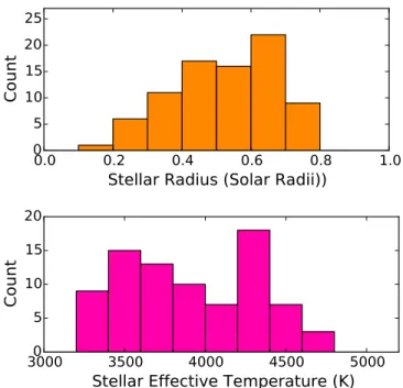
Figure 12.Distribution of radii(top) and effective temperatures (bottom) for the stars in our cool dwarf sample.
Table 6
Inferred Stellar Parameters for Low-mass Dwarfs
Teff(K) Radius(R) Mass(M) Luminosity(logL* L)
EPIC Date SpTypea Val −Err +Err Val −Err +Err Val −Err +Err Val −Err +Err 201205469 2015 Jun 13 K7V 3890 121 113 0.587 0.039 0.039 0.599 0.043 0.035 −1.178 0.188 0.175 201208431 2015 May 05 K7V 4015 173 155 0.569 0.047 0.049 0.635 0.046 0.035 −1.023 0.219 0.202 201345483 2015 May 05 M0V 4262 201 173 0.686 0.045 0.057 0.682 0.030 0.028 −0.630 0.218 0.198 201549860 2015 Nov 26 K4V 4403 96 93 0.620 0.028 0.029 0.702 0.013 0.013 −0.688 0.073 0.071 201617985 2015 Apr 16 M1V 3742 116 105 0.496 0.032 0.032 0.540 0.055 0.048 −1.480 0.141 0.134 201635569 2015 May 05 M0V 3970 118 112 0.623 0.032 0.032 0.623 0.035 0.028 −1.580 0.378 0.321 201637175 2015 May 05 K7V 3879 95 87 0.582 0.031 0.030 0.595 0.033 0.029 −1.258 0.135 0.124 201717274 2015 May 05 M2V 3286 134 130 0.314 0.057 0.054 0.194 0.159 0.133 −1.986 0.106 0.106 201855371 2015 Apr 16 K5V 4118 133 119 0.626 0.036 0.041 0.658 0.027 0.023 −0.845 0.142 0.133 205924614 2015 Sep 24 K7V 4423 149 130 0.700 0.045 0.056 0.705 0.018 0.022 −0.701 0.125 0.116 205924614b 2015 Nov 26 K7V 4300 107 100 0.715 0.040 0.043 0.688 0.015 0.015 −0.769 0.079 0.081 206011691 2015 Aug 07 K7V 4304 90 86 0.649 0.029 0.029 0.688 0.013 0.012 −1.111 0.072 0.071 206011691b 2015 Sep 24 K7V 4222 88 84 0.647 0.028 0.029 0.676 0.015 0.013 −1.235 0.082 0.083 206119924 2015 Sep 24 K7V 4348 86 88 0.669 0.030 0.030 0.695 0.013 0.012 −0.736 0.063 0.063 206209135 2015 Sep 24 M2V 3360 87 86 0.331 0.030 0.030 0.271 0.091 0.079 −1.872 0.059 0.058 206312951 2015 Sep 24 M1V 3707 80 81 0.478 0.028 0.028 0.523 0.045 0.037 −1.277 0.066 0.064 206318379 2015 Sep 24 M4V 3293 89 87 0.280 0.031 0.031 0.201 0.102 0.090 −1.929 0.059 0.061 210448987 2015 Nov 27 K3V 4674 141 131 0.635 0.032 0.035 0.745 0.023 0.034 −0.656 0.062 0.059 210489231 2015 Sep 24 M1V 4056 113 104 0.557 0.034 0.037 0.645 0.027 0.022 −0.937 0.067 0.063 210508766 2015 Sep 24 M1V 3876 81 80 0.547 0.028 0.028 0.594 0.031 0.025 −1.393 0.071 0.066 210558622b 2015 Oct 14 K7V 4268 105 98 0.678 0.036 0.040 0.683 0.016 0.015 −0.685 0.076 0.070 210558622 2015 Nov 26 K7V 4350 112 106 0.770 0.050 0.057 0.695 0.015 0.016 −0.590 0.076 0.070 210564155 2015 Nov 27 M2V 3344 90 87 0.286 0.031 0.030 0.255 0.093 0.084 −2.008 0.062 0.061 210707130 2015 Sep 24 K5V 4376 95 90 0.676 0.031 0.031 0.698 0.013 0.013 −0.711 0.063 0.062 210750726 2015 Sep 24 M1V 3624 88 87 0.460 0.030 0.032 0.477 0.057 0.048 −1.530 0.055 0.054 210838726 2015 Sep 24 M1V 3792 78 78 0.503 0.028 0.028 0.562 0.036 0.030 −1.371 0.058 0.057 210968143 2015 Sep 24 K5V 4422 93 91 0.635 0.029 0.029 0.705 0.013 0.013 −0.994 0.064 0.066 211077024 2015 Nov 26 M3V 3489 81 80 0.321 0.029 0.029 0.384 0.067 0.058 −1.742 0.054 0.054 211305568 2015 Nov 27 M1V 3612 85 84 0.446 0.030 0.031 0.470 0.056 0.048 −1.462 0.057 0.056 211331236 2015 Nov 26 M1V 3755 85 83 0.457 0.028 0.028 0.546 0.042 0.035 −1.358 0.061 0.059 211331236b 2016 Apr 18 M1V 3842 82 82 0.492 0.028 0.028 0.582 0.034 0.028 −1.262 0.060 0.060 211336288 2016 Mar 27 M0V 3997 80 79 0.586 0.027 0.027 0.630 0.022 0.019 −1.365 0.062 0.061 211357309 2015 Nov 27 M1V 3731 86 85 0.460 0.028 0.028 0.535 0.045 0.038 −1.402 0.060 0.059 211428897 2015 Nov 26 M2V 3595 95 91 0.290 0.030 0.030 0.459 0.064 0.055 −1.685 0.056 0.058 211509553 2016 Mar 27 M0V 3756 81 80 0.547 0.029 0.029 0.546 0.040 0.034 −1.592 0.087 0.081 211680698 2016 Mar 28 K3V 4726 143 127 0.735 0.043 0.047 0.756 0.025 0.039 −0.593 0.063 0.061 211694226a 2016 Mar 8 M3V 3454 83 82 0.445 0.031 0.031 0.356 0.074 0.064 −1.459 0.076 0.073 211694226b 2016 Mar 8 M3V 3448 93 92 0.440 0.035 0.037 0.351 0.084 0.072 −1.647 0.086 0.084 211762841 2016 Mar 4 K7V 4136 87 86 0.626 0.029 0.030 0.661 0.018 0.015 −1.080 0.078 0.075 211770795 2016 Apr 18 K5V 4753 155 129 0.679 0.036 0.038 0.763 0.027 0.046 −0.572 0.076 0.070 211791178 2016 Mar 27 M0V 4350 102 96 0.667 0.034 0.038 0.695 0.014 0.014 −0.669 0.068 0.068 211799258c 2016 Mar 8 M3V 3317 73 73 0.328 0.062 0.069 0.227 0.077 0.077 −2.117 0.373129 0.373129 211817229c 2016 Mar 4 M4V 3276 73 73 0.237 0.041 0.046 0.183 0.082 0.082 −2.279 0.676023 0.676023 211818569 2016 Feb 19 K5V 4471 112 104 0.768 0.042 0.042 0.712 0.014 0.017 −0.611 0.058 0.057 211822797 2016 Mar 27 K7V 4148 82 80 0.572 0.027 0.027 0.663 0.016 0.014 −1.218 0.061 0.061 211826814c 2016 Feb 19 M4V 3288 73 73 0.262 0.049 0.055 0.196 0.080 0.080 −2.226 0.539306 0.539306 211831378 2016 Apr 18 M0V 3748 115 101 0.548 0.031 0.031 0.543 0.052 0.047 −1.480 0.148 0.154 211839798 2016 Mar 4 M4V 3522 175 133 0.265 0.039 0.049 0.409 0.110 0.109 −2.134 0.067 0.065 211924657 2016 Mar 8 M3V 3421 106 98 0.322 0.036 0.041 0.327 0.095 0.085 −1.902 0.064 0.063 211965883 2016 Mar 27 M0V 4211 80 79 0.600 0.027 0.027 0.674 0.014 0.012 −1.110 0.061 0.060 211969807 2016 Mar 8 M1V 3546 99 95 0.492 0.032 0.032 0.427 0.072 0.063 −1.476 0.109 0.100 211970234 2016 Apr 18 M4V 3292 159 150 0.190 0.039 0.036 0.200 0.185 0.153 −2.371 0.111 0.101 211988320 2016 Mar 27 K7V 4284 84 84 0.641 0.028 0.029 0.685 0.013 0.012 −1.174 0.059 0.058 212006344b 2015 Nov 26 M0V 3993 78 76 0.591 0.027 0.027 0.630 0.022 0.018 −1.186 0.065 0.066 212006344 2016 Feb 19 M0V 3963 77 76 0.625 0.028 0.028 0.621 0.024 0.020 −1.150 0.066 0.069 212069861 2015 Nov 26 M0V 4076 83 81 0.571 0.028 0.028 0.649 0.019 0.016 −1.091 0.068 0.063 212154564 2016 Mar 27 M3V 3561 87 84 0.344 0.030 0.030 0.436 0.062 0.054 −1.643 0.058 0.058 212354731 2016 Mar 28 M3V 3591 119 106 0.418 0.032 0.033 0.457 0.075 0.068 −1.531 0.096 0.091 212398486 2016 Mar 4 M2V 3654 100 92 0.402 0.031 0.031 0.495 0.057 0.051 −1.540 0.067 0.064 212443973 2016 Mar 27 M3V 3423 84 84 0.343 0.028 0.028 0.330 0.079 0.069 −1.888 0.054 0.054 212460519 2016 Mar 8 K7V 4368 128 115 0.621 0.034 0.036 0.697 0.016 0.018 −0.816 0.080 0.075 212554013 2016 Apr 18 K3V 4388 142 137 0.677 0.045 0.052 0.700 0.019 0.020 −0.757 0.080 0.078 212565386 2016 Mar 10 M1V 4342 159 137 0.581 0.036 0.041 0.694 0.020 0.022 −1.058 0.075 0.074
from the EWs. The latter use Teff and metallicity to estimate
radii indirectly; for Teff,we use the K-band temperatures (which
we refer to as “Mann temperatures,” see Section 4.2.1). The Mann et al. (2015) temperature–metallicity–radius relation is valid for stars with temperatures between 2700 and 4100 K, but many of the stars in our sample are hotter than this upper limit. For the stars for which the Mann et al. (2015) relations yield temperatures hotter than 4100 K, we instead compare the Newton et al.(2015) radii to the radii estimated by applying the temperature–radius relation provided in Equation (8) of Boyajian et al. (2012) using the Mann temperatures.
We display the resulting radius estimates in Figure 9. The Mann et al.(2015) methodology and the Newton et al. (2015) routines yield similar radii: the median radius difference is 0.01
R (the Mann radii are larger) and the standard deviation of the
differences is 0.06R. For comparison, the median reported
radius errors are 0.03 R for the Newton et al.(2015) values
and 0.05Rfor the Mann et al.(2015) values. Looking at the
hotter stars, the median difference between the Newton radii and Boyajian et al. (2012) radii is only 0.002 R and the
standard deviation of the difference is 0.05R
As shown in Figure 10, the primary reason why the temperature agreement looks worse for the coolest stars is because three cool stars(EPIC 211817229, EPIC 211799258, and EPIC 211826814) have significantly different parameters using the two methods. Based on the sample of stars with interferometrically constrained properties, the expected temperatures and radii of M5.5–M3dwarfs are 3054–3412K and 0.14–0.41 R, respectively (Boyajian et al. 2012).
Although these stars were visually classified as M3 or M4dwarfs, the Newton et al. (2015) routines assigned them high temperatures of 3594–3869 K because the Al-a EW measured in their spectra were below the lower limit of the calibration sample(see Table 7 for EW measurements). The Mann routines assigned the stars cooler temperatures of 3276–3317 K. Due to the better agreement between the Mann temperatures and expected temperatures of mid-M dwarfs, we chose to adopt the Mann et al. classifications for those three stars.
4.2.4. Stellar Luminosities
We compared the stellar luminosities estimated using the EW-based relation from Newton et al. (2015) to those found using the temperature–luminosity relation from Mann et al. (2013b). Due to the functional nature of the Mann et al. (2013b) relation, the Mann values followed a single track whereas the Newton values displayed scatter about that relation. Ignoring the three mid-M dwarfs that are too cool for the Newton relations, the luminosity differences(Newton– Mann) have a median value of 0.008L and a standard
deviation of 0.05 L. The scatter increases as temperature
increases. Dividing the sample into stars hotter and cooler than 4000K, the luminosity differences for cooler sample have a median value of 0.005Land a standard deviation of 0.03L
while the hotter sample has a median value of 0.034Land a
standard deviation of 0.07L. In the left panel of Figure11, we
display the adopted luminosities as a function of effective temperature.
Table 6 (Continued)
Teff(K) Radius(R) Mass(M) Luminosity(logL* L)
EPIC Date SpTypea Val −Err +Err Val −Err +Err Val −Err +Err Val −Err +Err 212572452 2016 Mar 27 K7V 4390 193 160 0.662 0.043 0.053 0.700 0.023 0.028 −0.807 0.165 0.155 212572452b 2016 Mar 10 K7V 4332 135 121 0.678 0.037 0.044 0.692 0.018 0.019 −0.854 0.128 0.120 212628098 2016 Apr 18 K7V 3942 84 82 0.566 0.028 0.028 0.615 0.027 0.022 −0.796 0.067 0.065 212634172 2016 Mar 4 M3V 3412 98 94 0.348 0.033 0.034 0.320 0.092 0.081 −1.866 0.064 0.062 212679181 2016 Mar 4 M3V 3616 89 87 0.434 0.029 0.029 0.472 0.058 0.050 −1.544 0.056 0.058 212679798 2016 Apr 18 M0V 3823 92 89 0.562 0.029 0.029 0.575 0.039 0.032 −1.009 0.081 0.084 212686205 2016 Mar 8 K4V 4470 172 145 0.778 0.061 0.076 0.711 0.020 0.028 −0.673 0.066 0.065 212690867 2016 Mar 8 M2V 3614 118 107 0.415 0.032 0.033 0.471 0.073 0.064 −1.603 0.078 0.077 212773272 2016 Apr 18 M3V 3367 82 81 0.428 0.030 0.030 0.277 0.084 0.074 −1.753 0.067 0.069 212773309 2016 Mar 28 M0V 4178 90 87 0.588 0.029 0.029 0.669 0.016 0.014 −0.797 0.056 0.057 212773309B 2016 Mar 28 M3V 3459 103 100 0.396 0.034 0.034 0.360 0.090 0.078 −1.632 0.097 0.104 213951550 2016 May 6 M3V 3574 88 85 0.471 0.030 0.030 0.445 0.061 0.054 −1.367 0.075 0.076 214254518b 2016 May 5 K7V 4335 102 94 0.668 0.033 0.037 0.693 0.014 0.014 −0.836 0.066 0.066 214254518 2016 Oct 26 K7V 4574 130 110 0.710 0.036 0.038 0.727 0.017 0.024 −0.758 0.065 0.067 214522613 2016 May 5 M1V 3602 99 94 0.448 0.032 0.032 0.463 0.065 0.056 −1.412 0.084 0.080 214787262 2016 May 5 M3V 3459 89 84 0.360 0.030 0.031 0.360 0.074 0.068 −1.841 0.056 0.055 216892056 2016 May 5 M2V 3467 84 82 0.398 0.029 0.029 0.367 0.071 0.063 −1.707 0.057 0.056 217941732 2016 May 5 K5V 4470 211 202 0.731 0.072 0.111 0.711 0.028 0.035 −0.844 0.153 0.116 217941732b 2016 Oct 26 K5V 4356 197 172 0.744 0.078 0.111 0.696 0.026 0.028 −0.858 0.132 0.126 Notes. a
Spectral types are coarse assignments based on visual inspection of the near-infrared spectra collected in this paper. The assigned spectral types have errors of roughly±1 subtype. (See Section4.1for details.)
b
Star observed twice to check the repeatability of our analysis. These are the higher precision estimates.
cThe Al-a EW for these stars are below the calibration range for the Newton et al.(2015) relations. Adopted parameters are based on the Mann et al. (2013a,2013b,
Table 7
Equivalent Widths and Metallicities for Cool Dwarfs
EW of Mg Features(A) EW of Al Features(A) Metallicitya (1.50 μm) (1.57 μm) (1.71 μm) a(1.67 μm) b(1.67 μm) [Fe/H] [M/H] EPIC Date Val Err Val Err Val Err Val Err Val Err Val Err Val Err 201205469 2015 Jun 13 5.84 0.37 3.82 0.30 3.59 0.33 2.43 0.21 3.01 0.23 0.433 0.166 0.307 0.146 201208431 2015 May 05 7.76 0.33 2.87 0.59 3.52 0.32 1.43 0.27 2.74 0.35 0.066 0.191 −0.024 0.170 201345483 2015 May 05 8.23 0.41 6.14 0.51 3.79 0.39 1.94 0.23 2.36 0.31 0.316 0.202 0.130 0.164 201549860 2015 Nov 26 8.13 0.10 5.08 0.10 3.86 0.09 1.72 0.07 2.15 0.09 L L L L 201617985 2015 Apr 16 5.26 0.26 3.35 0.22 4.29 0.20 1.56 0.15 2.60 0.20 −0.010 0.143 −0.022 0.116 201635569 2015 May 05 7.44 0.39 5.13 0.30 5.02 0.36 2.08 0.20 2.92 0.25 0.196 0.180 0.138 0.147 201637175 2015 May 05 7.00 0.21 4.53 0.22 4.32 0.18 2.14 0.13 3.03 0.19 0.032 0.125 0.007 0.108 201717274 2015 May 05 2.28 0.32 1.06 0.32 1.42 0.32 1.52 0.23 2.10 0.26 −0.257 0.154 −0.188 0.132 201855371 2015 Apr 16 8.15 0.25 5.33 0.26 4.00 0.21 1.42 0.15 2.41 0.19 L L L L 205924614 2015 Sep 24 8.30 0.22 5.81 0.20 4.17 0.17 1.39 0.13 2.17 0.16 0.246 0.125 0.170 0.108 205924614 2015 Nov 26 7.94 0.12 5.50 0.12 3.80 0.10 1.36 0.08 2.21 0.11 0.376 0.095 0.168 0.089 206011691 2015 Aug 07 8.13 0.08 5.60 0.08 4.42 0.07 1.66 0.06 2.33 0.09 −0.121 0.088 −0.122 0.085 206011691 2015 Sep 24 7.85 0.08 5.78 0.10 4.47 0.08 1.73 0.06 2.25 0.09 −0.034 0.090 −0.057 0.086 206119924 2015 Sep 24 8.34 0.07 5.68 0.08 3.88 0.06 1.52 0.06 2.25 0.08 0.337 0.086 0.204 0.084 206209135 2015 Sep 24 2.54 0.12 1.65 0.11 2.30 0.10 1.36 0.07 1.54 0.10 −0.271 0.093 −0.278 0.089 206312951 2015 Sep 24 4.95 0.11 3.28 0.11 3.10 0.09 1.64 0.07 2.39 0.08 0.097 0.092 0.066 0.087 206318379 2015 Sep 24 2.33 0.13 1.41 0.12 1.96 0.11 1.26 0.08 1.64 0.10 0.332 0.096 0.208 0.090 210448987 2015 Nov 27 7.41 0.10 4.88 0.10 3.14 0.09 1.39 0.07 1.59 0.10 L L L L 210489231 2015 Sep 24 6.32 0.12 3.63 0.12 3.16 0.11 1.24 0.09 1.99 0.13 0.524 0.098 0.349 0.091 210508766 2015 Sep 24 5.82 0.08 4.28 0.09 3.95 0.08 1.72 0.07 2.21 0.09 −0.107 0.089 −0.060 0.085 210558622 2015 Oct 14 8.16 0.10 5.45 0.12 3.81 0.10 1.42 0.09 2.37 0.11 0.025 0.096 0.012 0.089 210558622 2015 Nov 26 8.21 0.11 5.58 0.11 3.76 0.10 1.22 0.08 2.14 0.11 0.094 0.094 0.050 0.090 210564155 2015 Nov 27 2.00 0.11 1.39 0.11 1.53 0.10 1.20 0.08 1.44 0.10 −0.149 0.092 −0.124 0.088 210707130 2015 Sep 24 8.48 0.07 5.71 0.07 3.84 0.06 1.57 0.06 2.22 0.09 L L L L 210750726 2015 Sep 24 3.67 0.08 2.87 0.08 2.64 0.07 1.32 0.07 1.80 0.10 0.100 0.088 0.034 0.085 210838726 2015 Sep 24 5.28 0.06 3.55 0.08 3.51 0.07 1.63 0.05 2.21 0.07 0.180 0.085 0.111 0.083 210968143 2015 Sep 24 7.93 0.07 5.39 0.08 4.03 0.06 1.59 0.06 2.02 0.08 L L L L 211077024 2015 Nov 26 2.96 0.08 1.73 0.08 1.79 0.08 1.22 0.05 1.62 0.07 0.170 0.087 0.062 0.085 211305568 2015 Nov 27 3.99 0.09 2.89 0.09 2.79 0.08 1.23 0.07 1.96 0.10 −0.175 0.090 −0.105 0.087 211331236 2015 Nov 26 4.68 0.10 2.97 0.10 3.05 0.09 1.59 0.07 2.02 0.10 0.037 0.091 0.083 0.088 211331236 2016 Apr 18 5.02 0.11 3.23 0.09 3.19 0.07 1.93 0.07 2.28 0.10 0.106 0.088 −0.001 0.085 211336288 2016 Mar 27 6.42 0.08 4.76 0.06 4.05 0.05 1.81 0.05 2.33 0.08 −0.075 0.084 −0.123 0.084 211357309 2015 Nov 27 4.49 0.10 3.23 0.10 2.88 0.09 1.65 0.08 2.03 0.11 −0.175 0.092 −0.085 0.088 211428897 2015 Nov 26 3.19 0.10 1.59 0.10 1.87 0.09 1.13 0.07 1.46 0.09 −0.131 0.087 −0.154 0.085 211509553 2016 Mar 27 5.77 0.17 3.64 0.11 4.03 0.09 2.17 0.07 2.83 0.11 0.044 0.096 −0.177 0.092 211680698 2016 Mar 28 7.44 0.14 4.87 0.09 2.77 0.07 1.15 0.07 1.56 0.09 L L L L 211694226a 2016 Mar 8 4.13 0.18 2.98 0.17 2.83 0.17 1.67 0.12 2.74 0.13 0.043 0.108 0.053 0.101 211694226b 2016 Mar 8 3.54 0.24 2.75 0.22 2.39 0.24 1.71 0.15 2.42 0.16 0.261 0.131 0.117 0.110 211762841 2016 Mar 4 7.63 0.09 5.21 0.09 4.06 0.09 1.62 0.07 2.36 0.10 0.218 0.089 0.241 0.086 211770795 2016 Apr 18 7.38 0.17 5.35 0.12 3.27 0.09 1.33 0.07 1.54 0.10 L L L L 211791178 2016 Mar 27 7.30 0.15 4.79 0.11 3.24 0.09 1.26 0.06 1.79 0.07 −0.399 0.096 −0.095 0.092 211799258 2016 Mar 8 3.58 0.39 2.18 0.32 1.15 0.35 0.73 0.23 1.07 0.25 0.120 0.167 0.181 0.145 211817229 2016 Mar 4 1.23 0.12 0.90 0.11 0.95 0.11 0.63 0.08 0.62 0.11 −0.401 0.090 −0.327 0.088 211818569 2016 Feb 19 7.66 0.10 5.30 0.08 3.22 0.06 1.12 0.06 1.73 0.09 L L L L 211822797 2016 Mar 27 6.41 0.08 4.64 0.07 3.94 0.06 1.90 0.05 2.08 0.07 0.322 0.084 0.179 0.083 211826814 2016 Feb 19 2.60 0.35 0.97 0.27 1.33 0.21 0.63 0.15 1.06 0.19 −0.254 0.130 −0.317 0.123 211831378 2016 Apr 18 5.47 0.40 3.91 0.23 3.76 0.19 1.88 0.13 2.60 0.16 0.257 0.138 0.111 0.128 211839798 2016 Mar 4 1.69 0.12 1.18 0.12 1.48 0.12 0.92 0.08 0.98 0.11 −0.078 0.095 −0.010 0.089 211924657 2016 Mar 8 2.42 0.13 1.69 0.13 1.72 0.13 1.01 0.09 1.32 0.11 −0.004 0.096 −0.006 0.091 211965883 2016 Mar 27 7.40 0.08 5.10 0.07 4.16 0.05 1.86 0.04 2.33 0.06 −0.196 0.084 0.024 0.083 211969807 2016 Mar 8 3.87 0.25 3.47 0.21 3.26 0.23 1.73 0.15 2.67 0.18 0.179 0.125 0.200 0.116 211970234 2016 Apr 18 1.46 0.28 1.08 0.16 1.22 0.13 1.05 0.09 0.83 0.12 −0.177 0.109 −0.087 0.102 211988320 2016 Mar 27 7.20 0.08 5.13 0.06 4.20 0.04 1.50 0.04 1.97 0.06 −0.369 0.084 −0.157 0.083 212006344 2015 Nov 26 7.30 0.07 4.95 0.07 4.35 0.06 1.99 0.06 2.86 0.08 0.444 0.085 0.341 0.083 212006344 2016 Feb 19 7.25 0.10 5.38 0.09 4.12 0.06 2.37 0.06 3.15 0.08 0.521 0.086 0.309 0.085 212069861 2015 Nov 26 7.08 0.08 4.64 0.08 3.90 0.07 1.75 0.06 2.38 0.09 0.324 0.088 0.195 0.085 212154564 2016 Mar 27 3.35 0.11 2.00 0.10 2.63 0.07 1.14 0.05 1.64 0.07 −0.093 0.088 −0.238 0.086 212354731 2016 Mar 28 3.36 0.30 2.61 0.17 2.13 0.15 1.39 0.11 1.79 0.11 −0.009 0.124 0.018 0.107 212398486 2016 Mar 4 4.09 0.16 2.58 0.15 2.50 0.17 1.58 0.10 1.61 0.12 −0.278 0.103 −0.197 0.096 212443973 2016 Mar 27 2.31 0.08 1.99 0.06 2.44 0.05 1.12 0.05 1.32 0.08 0.201 0.084 −0.054 0.083 212460519 2016 Mar 8 7.57 0.11 4.77 0.12 3.68 0.11 1.42 0.10 1.71 0.13 −0.116 0.095 −0.140 0.091