Multi-object shape estimation and tracking from silhouette cues

HAL Id: inria-00349114

https://hal.inria.fr/inria-00349114

Submitted on 23 Dec 2008

HAL is a multi-disciplinary open access

archive for the deposit and dissemination of

sci-entific research documents, whether they are

pub-lished or not. The documents may come from

teaching and research institutions in France or

abroad, or from public or private research centers.

L’archive ouverte pluridisciplinaire HAL, est

destinée au dépôt et à la diffusion de documents

scientifiques de niveau recherche, publiés ou non,

émanant des établissements d’enseignement et de

recherche français ou étrangers, des laboratoires

publics ou privés.

Multi-object shape estimation and tracking from

silhouette cues

Li Guan, Jean-Sébastien Franco, Marc Pollefeys

To cite this version:

Li Guan, Jean-Sébastien Franco, Marc Pollefeys. Multi-object shape estimation and tracking from

silhouette cues. IEEE Conference on Computer Vision and Pattern Recognition, 2008. CVPR 2008.,

Jun 2008, Anchorage, United States. pp.1–8, �10.1109/CVPR.2008.4587786�. �inria-00349114�

Multi-Object Shape Estimation and Tracking from Silhouette Cues

Li Guan

UNC-Chapel Hill, U.S.A.

ETH-Z¨urich, Switzerland

lguan@cs.unc.edu

Jean-S´ebastien Franco

LaBRI - INRIA Sud-Ouest

University of Bordeaux, France

jean-sebastien.franco@labri.fr

Marc Pollefeys

UNC-Chapel Hill, U.S.A.

ETH-Z¨urich, Switzerland

marc@cs.unc.edu

Abstract

This paper deals with the 3D shape estimation from sil-houette cues of multiple moving objects in general indoor or outdoor 3D scenes with potential static obstacles, us-ing multiple calibrated video streams. Most shape-from-silhouette techniques use a two-classification of space oc-cupancy and silhouettes, based on image regions that match or disagree with a static background appearance model. Bi-nary silhouette information becomes insufficient to unam-biguously carve 3D space regions as the number and den-sity of dynamic objects increases. In such difficult scenes, multi-view stereo methods suffer from visibility problems, and rely on color calibration procedures tedious to achieve outdoors. We propose a new algorithm to automatically de-tect and reconstruct scenes with a variable number of dy-namic objects. Our formulation distinguishes between m different shapes in the scene by using automatically learnt view-specific appearance models, eliminating the color cal-ibration requirement. Bayesian reasoning is then applied to solve the m-shape occupancy problem, with m updated as objects enter or leave the scene. Results show that this method yields multiple silhouette-based estimates that dras-tically improve scene reconstructions over traditional two-label silhouette scene analysis. This enables the method to also efficiently deal with multi-person tracking problems.

1. Introduction

Shape modeling from video is an important computer vi-sion problem with numerous applications, such as 3D pho-tography, virtual reality, 3D interaction or markerless mo-tion capture. Silhouette-based techniques [13,1] have been popularized thanks to their simplicity, speed, and general robustness to provide global shape and topology informa-tion about objects. Multi-view stereo techniques [12,3,17] prove more precise as they additionally recover object con-cavities, but are generally more computationally intense and require object appearance to be similar across views. The success of both families of approaches largely relies on the amount of control over the acquired scene, and is chal-lenged in general, outdoor, densely populated scenes, where assumptions about visibility, lighting and scene content

break. Primitive extraction and color calibration, both nec-essary for inter-view photocorrelation, become challenging or impossible. Binary silhouette reasoning with several ob-jects is prone to large visual ambiguities, leading to mis-classifications of significant portions of 3D space. Occlu-sion may occur between dynamic objects of interest. It can also be introduced by static objects in the scene, whose ap-pearances are learned as part of the background model in many approaches, including ours. These occluders result in ambiguous and partial silhouette extractions.

In this paper we show that silhouette reasoning can be efficiently conducted by using distinct appearance models for objects, yielding a multi-silhouette modeling approach. We propose a Bayesian framework to merge silhouette cues arising from a set of dynamic objects, which accounts for all types of object occlusions and additional object localiza-tion constraints. This approach is shown to improve shape-from-silhouette estimation, can naturally be integrated with existing probabilistic occlusion inference methods, and can naturally benefit other vision problems such as multi-view tracking, segmentation, and general 3D modeling.

1.1. Previous work

Silhouette-based modeling in calibrated multi-view se-quences has been largely popular, and yielded a large num-ber of approaches to build volume-based [21] or surface-based [1] representations of the object’s visual hull. The dif-ficulty and focus in attention in modeling objects from sil-houettes has gradually shifted from the pure 3D reconstruc-tion issue to the sensitivity of visual hull representareconstruc-tions to silhouette noise. In fully automatic modeling systems, sil-houettes are usually extracted using background subtraction techniques [20,4], which are difficult to apply outdoors and often locally fail due to changing lighting conditions, shad-ows, color space ambiguities, background object induced occlusion, among other causes. Several solutions have been proposed to address these problems, using a discrete op-timization scheme [19], silhouette priors over multi-view sets [9], or silhouette cue integration using a sensor fusion paradigm [7]. Most existing reconstruction methods how-ever focus on mono-object situations, and fail to address the specific multi-object issues of silhouette methods.

(a) (b)

Figure 1. The principle of multi-object silhouette reasoning for shape modeling disambiguation. Best viewed in color.

While inclusive of the object’s shape [13], visual hulls fail to capture object concavities but are usually very good at hinting toward the overall topology of a single observed object, a property that has been successfully used in a number of photometric-based methods to carve an initial silhouette-based volume [18,8].

This ability to capture topologies breaks with the multi-plicity of objects in the scene. In such cases 2-silhouettes are ambiguous in distinguishing between regions actually occupied by objects and unfortunate silhouette-consistent “ghost” regions. Such regions have been analyzed in the context of tracking applications to avoid committing to a “ghost” track [16]. The method we propose casts the prob-lem of silhouette modeling at the multi-object level, where ghosts can naturally be eliminated based on per object sil-houette consistency. Multi-object silsil-houette reasoning has been applied in the context of multi-object tracking [15,6]. The reconstruction and occlusion problem has also been studied for the specific case of transparent objects [2]. Re-cent tracking efforts also use 2D probabilistic occlusion rea-soning to improve object localization [11]. Static occluder analysis has also been proposed to analyze 3D scenes [10]. Our work is more general as it estimates full 3D shapes and copes with 3D occlusions both dynamic and static.

Perhaps the closest related work is the approach of Ziegler et al. [22], which builds 3D models deterministi-cally from multiple label, user-provided silhouette segmen-tations. The approach we propose produces a more general probabilistic model that accounts for process noise and re-quires little or no user intervention.

1.2. Principle

The ghost phenomenon occurs when the configuration of the scene is such that regions of space occupied by ob-jects of interest cannot be disambiguated from free-space regions that also happen to project inside all silhouettes, as the polygonal gray region in Fig.1.2(a). Ghosts are increas-ingly likely as the number of observed objects rises, because it then becomes more difficult to find views that visually separate objects in the scene and carve out unoccupied re-gions of space. This problem is even aggravated for ro-bust schemes, such as [7,10], which do not strictly require silhouettes to be observed in every view. To address this problem, we initialize and learn a set of view-specific

ap-pearance models associated to m objects in the scene. The intuition is then that the probability of confusing ambiguous regions with real objects decreases, because the silhouette set corresponding to ghosts is then drawn from non object-consistent appearance model sets, as depicted in Fig.1.2(b). It is possible to process multiple silhouette labels in a deterministic, purely geometric fashion [22], but this comes at the expense of an arbitrary hard threshold for the num-ber of views that define consistency. Silhouettes are then also assumed to be manually given and noiseless, which cannot be assumed for automatic processing. Using a vol-ume representation of the 3D scene, we thus process multi-object sequences by examining each voxel in the scene us-ing a Bayesian formulation (§2), which encodes the noisy causal relationship between the voxel and the pixels that observe it in a generative sensor model. In particular, given the knowledge that a voxel is occupied by a certain object among m possible in the scene, the sensor model explains what appearance distributions we are supposed to observe, corresponding to that object. It also encodes state informa-tion about the viewing line and potential obstrucinforma-tions from other objects, as well as a localization prior used to enforce the compactness of objects, which can be used to refine the estimate for a given instant of the sequence. Voxel sensor model semantics and simplifications are borrowed from the occupancy grid framework explored in the robotics com-munity [5,14]. The proposed method can also be seen as a multi-object generalization of previous probabilistic ap-proaches focused on 2-label silhouette modeling [7,10].

This scheme enables us to perform silhouette inference (§2.3) in a way that reinforces regions of space which are drawn from the same conjunction of color distributions, corresponding to one object, and penalizes appearance in-consistent regions, while accounting for object visibility. An algorithm (§3) is then proposed to integrate the infer-ence framework in a fully automatic system. Because they are mutually dependent, specific steps are proposed for the problems of initialization, appearance model estimation, multi-object and occluder shape recovery.

2. Formulation

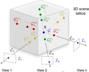
We consider a scene observed by n calibrated cameras. We assume a maximum of m dynamic objects of interest can be present in the scene. In this formulation we focus on the state of one voxel at position X chosen among the positions of the 3D lattice used to discretize the scene. We here model how knowledge about the occupancy state of voxel X influences image formation, assuming a static ap-pearance model for the background has previously been ob-served. Because of occlusion relationships arising between objects, the zones of interest to infer the state of voxel X are its n viewing linesLi, i∈ {1, · · · , n}, with respect to

Gv₁ 1 Gv₂ 1 Gvm 1 Gv₁ 2 Gv₂ 2 Gvm 2 Gv₁ n Gv₂ n Gvm n View 2 3D scene lattice X View 1 ... View n · · · ·_· · · ·· G I_{1 I} 2 In L₁ L₂ Ln

Figure 2. Overview of main statistical variables and geometry of the problem. G is the occupancy at voxel X and lives in a state spaceL of object labels. {Ii} are the color states observed at the npixels where X projects. {G_ivj} are the states in L of the most likely obstructing voxels on the viewing line, for each of the m objects, enumerated in their order of visibility{vj}i.

prior knowledge about scene state is available for each voxel X in the lattice and can be used in the inference. Various uses of this assumption will be demonstrated in§3. A num-ber of statistical variables are used to model the state of the scene, the image generation process and to inferG, as de-picted in figure Fig.2.

2.1. Statistical Variables

Scene voxel state space. The occupancy state of X is represented by a variableG. The particularity of our mod-eling lies in the multi-labmod-eling characteristic of G ∈ L, whereL is a set of labels {∅, 1, · · · , m, U}. A voxel is ei-ther empty (∅), one of m objects the model is keeping track of (numerical labels), or occupied by an unidentified object (U). U is intended to act as a default label capturing all ob-jects that are detected as different than background but not explicitly modeled by other labels, which proves useful for automatic detection of new objects (§3.3).

Observed appearance. The voxel X projects to a set of pixels, whose colorsIi, i ∈ 1, · · · , n we observe in

im-ages. We assume these colors are drawn from a set of object and view specific color models whose parameters we note Cl

i. More complex appearance models are possible using

gradient or texture information, without loss of generality. Latent viewing line variables. To account for inter-object occlusion, we need to model the contents of view-ing lines and how it contributes to image formation. We assume some a priori knowledge about where objects lie in the scene. The presence of such objects can have an impact on the inference ofG because of the visibility of objects and

how they affectG. Intuitively, conclusive information about G cannot be obtained from a view i if a voxel in front of G with respect to i is occupied by another object, for exam-ple. However,G directly influences the color observed if it is unoccluded and occupied by one of the objects. But ifG is known to be empty, then the color observed at pixel Ii

reflects the appearance of objects behind X in image i, if any. These visibility intuitions are modeled below (§2.2).

It is not meaningful to account for the combinatorial number of occupancy possibilities along the viewing rays of X. This is because neighboring voxel occupancies on the viewing line usually reflect the presence of the same object and are therefore correlated. In fact, assuming we witness no more than one instance of every one of the m objects along the viewing line, the fundamental informa-tion that is required to reason about X is the knowledge of presence and ordering of the objects along this line. To rep-resent this knowledge, as depicted in Fig.2, assuming prior information about occupancies is already available at each voxel, we extract, for each label l ∈ L and each viewing line i ∈ {1, · · · , n}, the voxel whose probability of occu-pancy is dominant for that label on the viewing line. This corresponds to electing the voxels which best represent the m objects and have the most influence on the inference of G. We then account for this knowledge in the problem of inferring X, by introducing a set of statistical occupancy variablesGl

i ∈ L, corresponding to these extracted voxels.

2.2. Dependencies Considered

We propose a set of simplifications in the joint prob-ability distribution of the set of variables, that reflect the prior knowledge we have about the problem. To simplify the writing we will often note the conjunction of a set of variables as following: G1:m

1:n = {Gli}i∈{1,··· ,n},l∈{1,··· ,m}.

We propose the following decomposition for the joint prob-ability distribution p(G G1:m 1:n I1:nC1:n1:m): p(G)Y l∈L p(Cl 1:n) Y i,l∈L p(Gl i|G) Y i p(Ii|G Gi1:mC 1:m i ) (1)

Prior terms. p(G) carries prior information about the current voxel. This prior can reflect different types of knowledge and constraints already acquired about G, e.g. localization information to guide the inference (§3).

p(Cl

1:n) is the prior over the view-specific appearance

models of a given object l. The prior, as written over the conjunction of these parameters, could express expected relationships between the appearance models of different views, even if not color-calibrated. Since the focus in this paper is on the learning of voxel X, we do not use this ca-pability here and assume p(Cl

1:n) to be uniform.

Viewing line dependency terms. We have summarized the prior information along each viewing line using the m

voxels most representative of the m objects, so as to model inter-object occlusion phenomena. However when examin-ing a particular labelG = l, keeping the occupancy infor-mation aboutGl

i would lead us to account for intra-object

occlusion phenomena, which in effect would lead the infer-ence to favor mostly voxels from the front visible surface of the object l. Because we wish to model the volume of object l, we discard the influence ofGl

iwhenG = l:

p(Gk

i|{G = l}) = P(Gik) when k6= l (2)

p(Gil|{G = l}) = δ∅(Gil) ∀l ∈ L, (3)

whereP(Gk

i) is a distribution reflecting the prior

knowl-edge aboutGk

i, and δ∅(Gik) is the distribution giving all the

weight to label∅. In (3) p(Gl

i|{G = l}) is thus enforced to

be empty whenG is known to be representing label l, which ensures that the same object is represented only once on the viewing line.

Image formation terms. The image formation term p(Ii|G Gi1:m C

1:m

i ) explains what color we expect to

ob-serve given the knowledge of viewing line states and per-object color models. We decompose each such term in two subterms, by introducing a local latent variableS ∈ L rep-resenting the hidden silhouette state:

p(Ii|G Gi1:mC 1:m i ) = X S p(Ii|S Ci1:m)p(S|G G 1:m i ) (4)

The term p(Ii|S Ci1:m) simply describes what color is

likely to be observed in the image given the knowledge of the silhouette state and the appearance models correspond-ing to each object. S acts as a mixture label: if {S = l} then Ii is drawn from the color model Cil. For objects

(l∈ {1, · · · , m}) we typically use Gaussian Mixture Mod-els (GMM) [20] to efficiently summarize the appearance in-formation of dynamic object silhouettes. For background (l = ∅) we use per-pixel Gaussians as learned from pre-observed sequences, although other models are possible. When l = U the color is drawn from the uniform distri-bution, as we make no assumption about the color of previ-ously unobserved objects.

Defining the silhouette formation term p(S|G G1:m i )

re-quires that the variables be considered in their visibility or-der, to model the occlusion possibilities. Note that this order can be different from1, · · · , m. We note {Gvj

i }j∈{1,··· ,m}

the variablesG1:m

i as enumerated in the permutated order

{vj}ireflecting their visibility ordering onLi. If{g}i

de-notes the particular index after which the voxel X itself ap-pears onLi, then we can re-write the silhouette formation

term as p(S|Gv1 i · · · G vg i G G vg+1 i · · · G vm i ). A distribution

of the following form can then be assigned to this term:

p(S|∅ · · · ∅ l ∗ · · ·∗) = dl(S) with l 6= ∅ (5)

p(S|∅ · · · ∅) = d∅(S), (6)

where dk(S), k ∈ L is a family of distributions

giv-ing strong weight to label k and lower equal weight to others, determined by a constant probability of detection Pd ∈ [0, 1]: dk(S = k) = Pdand dk(S 6= k) = _|L|−11−Pd to

ensure summation to1. (5) thus expresses that the silhouette pixel state reflects the state of the first visible non-empty voxel on the viewing line, regardless of the state of voxels behind it (“*”). (6) expresses the particular case where no occupied voxel lies on the viewing line, the only case where the state ofS should be background: d_∅(S) ensures that Ii

is mostly drawn from the background appearance model.

2.3. Inference

Estimating the occupancy at voxel X translates to esti-mating p(G|I1:nC1:n1:m) in Bayesian terms. We apply Bayes’

rule using the joint probability distribution, marginalizing out the unobserved variablesG1:m

1:n: p(G|I1:nC1:n1:m) = 1 z X G1:m 1:n p(G G1:n1:mI1:n C1:m1:n) (7) = 1 zp(G) n Y i=1 fi1 (8) where fik = X G_ivk p(Gvk i |G)f k+1 i for k < m (9) and fim= X Gvm i p(Gvm i |G)p(Ii|G Gi1:mC 1:m i ) (10)

The normalization constant z is easily obtained by ensuring summation to 1 of the distribution: z = P

G,G1:m 1:n p(G G

1:m

1:n I1:n C1:n1:m). (7) is the direct

applica-tion of Bayes rule, with the marginalizaapplica-tion of latent vari-ables. The sum in this form is intractable, thus we factorize the sum in (8). The sequence of m functions fk

i specify

how to recursively compute the marginalization with the sums of individual Gk

i variables appropriately subsumed,

so as to factor out terms not required at each level of the sum. Because of the particular form of silhouette terms in (5), this sum can be efficiently computed by noting that all terms after a first occupied voxel of the same visibility rank k share a term of identical value in p(Ii|∅ · · · ∅ {Givk =

l} ∗ · · · ∗) = Pl(Ii). They can be factored out of the

re-maining sum, which sums to1 being a sum of terms of a probability distribution, leading to the following simplifica-tion of (9),∀k ∈ {1, · · · , m − 1}: fik= p(G vk i = ∅|G)f k+1 i + X l6=∅ p(Gvk i = l|G)Pl(Ii) (11)

3. 3D Modeling and Localization Algorithm

likely it is for X to belong to one of m objects. Some addi-tional work is required to use it to model objects in practice. The formulation explains how to compute the occupancy of X if some occupancy information about the viewing lines is already known. Thus the algorithm needs to be initial-ized with a coarse shape estimate, whose computation is discussed in§3.1. Intuitively, object shape estimation and tracking are complementary and mutually helpful tasks. We explain in§3.2how object localization information is com-puted and used in the modeling. To be fully automatic, our method uses the inference labelU to detect objects not yet assigned to a given label and learn their appearance mod-els (§3.3). Finally, it has been shown that static occluders can be computed using silhouette occlusion reasoning [10]. This reasoning can easily be integrated in our approach and help the inference be robust to static occluders (§3.4). The algorithm at every time instance is summarized in Alg.1.

Algorithm 1: Dynamic Scene Reconstruction Input: Frames at a new time instance for all views Output: 3D object shapes in the scene

Coarse Inference;

1

if new object enters the scene then

2

add a label for the new object;

3

initialize foreground appearance model;

4

go to step1;

5

Refined Inference;

6

static occluder inference;

7

update object location and prior;

8

return

9

3.1. Shape Initialization and Refinement

The proposed formulation relies on some available prior knowledge about the scene occupancies and dynamic ob-ject ordering. Thus part of the occupancy problem must be solved to bootstrap the algorithm. Fortunately, using multi-label silhouette inference with no prior knowledge about oc-cupancies or consideration for inter-object occlusions pro-vides a decent initial m-occupancy estimate. This simpler inference case can easily be formulated by simplifying oc-clusion related variables from (8):

p(G|I1:n C1:m1:n) = 1 zp(G) n Y i=1 p(Ii|G Ci1:m) (12)

This initial coarse inference can then be used to infer a second, refined inference, this time accounting for viewing line obstructions, given the voxel priors p(G) and P(Gij) of

equation (2) computed from the coarse inference. The prior over p(G) is then used to introduce soft constraints to the in-ference. This is possible by using the coarse inference result as the input of a simple localization scheme, and using the localization information in p(G) to enforce a compactness prior over the m objects, as discussed in§3.2.

3.2. Object Localization

We use a localization prior to enforce the compactness of objects in the inference steps. For the particular case where walking people represent the dynamic objects, we take ad-vantage of the underlying structure of the dataset, by pro-jecting the maximum probability over a vertical voxel col-umn on the horizontal reference plane. We then localize the most likely position of objects by sliding a fixed-size win-dow over the resulting 2D probability map for each object. The resulting center is subsequently used to initialize p(G), using a cylindrical spatial prior. This favors objects local-ized in one and only one portion of the scene and is intended as a soft guide to the inference. Although simple, this track-ing scheme is shown to outperform state of the art methods (§4.2), thanks to the rich shape and occlusion information modelled.

3.3. Automatic Detection of New Objects

The main information about objects used by the pro-posed method is their set of appearances in the different views. These sets can be learned offline by segmenting each observed object alone in a clear, uncluttered scene be-fore processing multi-objects scenes. More generally, we can initialize object color models in the scene automatically. To detect new objects we computeU’s object location and volume size during the coarse inference, and track the un-known volume just like other objects as described in§3.2. A new dynamic object inference label is created (and m in-cremented), if all of the following criteria are satisfied:

• The entrance is only at the scene boundaries • U’s volume size is larger than a threshold • Subsequent updates of U’s track are bounded

To build the color model of the new object, we project the maximum voxel probability along the viewing ray to the camera view, threshold the image to form a “silhou-ette mask”, and choose pixels within the mask as training samples for a GMM appearance model. Samples are only collected from unoccluded silhouette portions of the object, which can be verified from the inference. Because the cam-eras may be badly color-calibrated, we propose to train an appearance model for each camera view separately. This approach is fully evaluated in§4.1.

3.4. Occluder computation

The existing algorithm in [10] computes dynamic object binary occupancy distributions at every voxel. It then an-alyzes the presence of dynamic object dominant probabil-ities of occupancy in front and behind of the voxel on its viewing lines, for every view and passed time instant of the sequence. Such dominant occupancies are then used to ac-cumulate cues about occluder occupancy at the current in-ferred voxel. The same formulation can easily be used and

extended using the analysis presented in this paper. At ev-ery time instant the dominant occupancy probabilities of m objects are already extracted; the two dominant occupan-cies in front and behind the current voxel X can be used in the occupancy inference formulation of [10]. The occlusion occupancy inference then benefits from the disambiguation inherent to multi-silhouette reasoning.

4. Results and Evaluations

We have used four multi-view sequences to validate our approach. Eight30Hz 720 × 480 DV cameras surrounding the scene in a semi-circle were used for theCLUSTERand

BENCH sequences. The LAB and SCULPTURE sequences

are provided by [11] and [10] respectively for comparison.

Cam. No. Dynamic Obj. No. Occluder

CLUSTER(outdoor) 8 5 no

BENCH(outdoor) 8 0 - 3 yes

LAB(indoor) 15 4 no

SCULPTURE(outdoor) 9 2 yes

Cameras in each data sequence are geometrically cali-brated but not color calicali-brated. The background model is learned per-view using a single Gaussian color model at every pixel, with training images. Although simple, the model proves sufficient, even in outdoor sequences subject to background motion, foreground object shadows, window reflections and substantial illumination changes, showing the robustness of the method to difficult real conditions.

For dynamic object appearance models of theCLUSTER,

LAB and SCULPTURE data sets, we train a RGB GMM

model for each person in each view with manually seg-mented foreground images. This is done offline. For the

BENCH sequence however, appearance models are

initial-ized online automatically.

The time complexity isO(nmV ), with n the number of cameras, m the number of objects in the scene, and V the scene volume resolution. We process the data sets on a2.4 GHz Core Quad PC with computation times varying of 1-4 min per time step. The very strong locality inherent to the algorithm and preliminary benchmarks suggest that around 10 times faster performance could be achieved using a GPU implementation. Please refer to the supplemental videos for complete results.

4.1. Appearance Modeling Validation

It is extremely hard to color-calibrate a large number of cameras, not to mention under varying lighting conditions, as in a natural outdoor environment. To show this, we com-pare different appearance modeling schemes in Fig.3, for a frame of the outdoor BENCH dataset. Without loss of generality, we use GMMs. The first two rows compare silhouette extraction probabilities using the color models

Figure 3. Appearance model analysis. A person in eight views is displayed in row 4. A GMM modelCi is trained for view i ∈ [1, 8]. A global GMM model C0 over all views is also trained. Row 1, 2, 3 and 5 compute P(S|I, B, Ci+1), P(S|I, B, Ci−1), P(S|I, B, C0) and P(S|I, B, Ci) for view i respectively, with S the foreground label,I the pixel color, B the uniform background model. The probability is displayed according to the color scheme at the top right corner. The average probability over all pixels in the silhouette region and the mean color modes of the applied GMM model are shown for each figure. Best viewed in color.

of spatially neighboring views. These indicate that stereo approaches which heavily depend on color correspondence between neighboring views are very likely to fail in the nat-ural scenarios, especially when the cameras have dramatic color variations, such as in view 4 and 5. The global appear-ance model on row 3 performs better than row 1 and 2, but this is mainly due to its compensation between large color variations across camera views, which at the same time, de-creases the model’s discriminability. The last row obviously is the winner where a color appearance model is indepen-dently maintained for every camera view. We hereby use the last scheme in our system. Once the model is trained, we do not update it as time goes by, which could be an easy extension for robustness.

4.2. Densely Populated Scene

The CLUSTER sequence is a particularly challenging

configuration: five people are on a circle of less than3m. in diameter, yielding an extremely ambiguous and occluded situation at the circle center. Despite the fact that none of them are being observed in all views, we are still able to re-cover the people’s label and shape. Images and results are shown in Fig.4. The naive2-label reconstruction (proba-bilistic visual hull) yields large volumes with little separa-tion between objects, because the entire scene configurasepara-tion

Figure 4. Result from 8-viewCLUSTERdataset. (a) Two views at frame 0. (b) Respective 2-labeled reconstruction. (c) More accu-rate shape estimation using our algorithm. Best viewed in color.

is too ambiguous. Adding tracking prior information es-timates the most probable compact regions and eliminates large errors, at the expense of dilation and lower precision. Accounting for viewing line occlusions enables the model to recover more detailed information, such as the limbs.

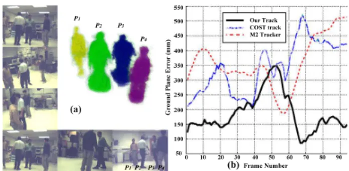
TheLABsequence [11] with poor image contrast is also processed. The reconstruction result from all 15 cameras is shown in Fig.5. Moreover, in order to evaluate our local-ization prior estimation, we compare our tracking method (§3.2) with the ground truth data, the result of [11] and [15]. We use the same8 cameras as in [15] for the comparison, shown in Fig.5(b). Although slower in its current imple-mentation (2 min. per time step) our method is generally more robust in tracking, and also builds 3D shape informa-tion. Most existing tracking methods only focus on a track-ing envelope and do not compute precise 3D shapes. This shape information is what enables our method to achieve comparable or better precision.

4.3. Automatic Appearance Model Initialization

The automatic dynamic object appearance model initial-ization has been tested using theBENCH sequence. Three people are walking into the empty scene one after another. By examining the unidentified labelU, object appearance models are initialized and used for shape estimation in sub-sequent frames. Volume size evolution of all labels are shown in Fig.6and the reconstructions at two time instants are shown in Fig.7.

During the sequence, U has three major volume peaks due to three new persons entering the scene. Some smaller perturbations are due to shadows on the bench or the ground. Besides automatic object appearance model initial-ization, the system robustly re-detects and tracks the person who leaves and re-enters the scene. This is because once the label is initialized, it is evaluated for every time instant, even if the person is out of the scene. The algorithm can easily be improved to handle leaving/reentering labels transparently.

Figure 5.LABdataset result from [11]. (a) 3D reconstruction with 15 views at frame 199 (b) 8-view tracking result comparison with methods in [11], [15] and the ground truth data. Mean error in ground plane estimate in mm is plotted. Best viewed in color.

Figure 6. Appearance model automatic initialization with the

BENCHsequence. The volume ofU increases if a new person en-ters the scene. When an appearance model is learned, a new label is initialized. During the sequence, L1 and L2 volumes drop to near zero because they walk out of the scene on those occasions.

Figure 7.BENCHresult. Person numbers are assigned according to the order their appearance models are initialized. At frame 329, P3is entering the scene. Since it’s P3’s first time into the scene, he is captured by labelU (gray color). P1is out of the scene at the moment. At frame 359, P1has re-entered the scene. P3has its GMM model already trained and label L3assigned. The bench as a static occluder is being recovered. Best viewed in color.

4.4. Dynamic Object & Occluder Inference

TheBENCHsequence demonstrates the power of our

au-tomatic appearance model initialization as well as the inte-grated occluder inference of the “bench” as shown in Fig.7

between frame 329 and 359. Check Fig.6about the scene configuration during that period. The complete sequence is also given in the supplemental video.

We also compute result forSCULPTUREsequence from [10] with two persons walking in the scene, as shown in Fig.8. For the dynamic objects, we manage to get much

Figure 8. SCULPTUREdata set comparison. While both [10] and our method recover the static sculpture, our method resolves inter-occlusion ambiguities, and estimates much better dynamic object shapes. Best viewed in color.

cleaner shapes when the two persons are close to each other, and more detailed shapes such as extended arms. For the occluder, we are able to recover the fine shape too, while [10] has a lot of noise, due to the occluder inference using ambiguous regions when people are clustered.

5. Discussion

We have proposed a Bayesian method to build 3D shapes from multi-object silhouette cues. The appearances of ob-jects are used to disambiguate free regions of space which project inside silhouettes, and occlusion information and object localization priors are used to update the represen-tation iteratively so as to refine the resulting shapes. Our results show that the shapes obtained using this approach yield significantly better results than pure silhouette reason-ing, which makes no distinction between different objects. This new multi-silhouette inference algorithm is robust to very difficult conditions, and can prove very useful for var-ious vision tasks such as tracking, localization and 3D re-construction, in highly cluttered scenes with densely packed dynamic object groups. A large number of extensions can be tested on the basis of the framework provided, including more general and complex appearance modeling, different enforcements of the compactness of objects, a more gen-eral management of objects entering and leaving the scene. It is possible to analyze object label transition, for exam-ple a static object in the scene might be moved to a differ-ent place, and a person might come and sit statically on the bench. Temporal consistency constraints could also be in-cluded in stronger forms, to enforce temporal continuity of the reconstruction and smoothness of the flow in the scene.

Acknowledgments: We would like to thank A. Gupta et.al. [11,15] for providing us the 16-camera dataset. This work was partially supported by David and Lucille Packard Foundation Fel-lowship, and NSF Career award IIS-0237533.

References

[1] B. G. Baumgart. Geometric Modeling for Computer Vision. PhD thesis, CS Dept, Stanford U., Oct. 1974.

[2] J. S. Bonet and P. Viola. Roxels: Responsibility weighted 3d volume reconstruction. In ICCV, vol. I, p. 418–425, 1999. [3] A. Broadhurst, T. Drummond, and R. Cipolla. A

probabilis-tic framework for the Space Carving algorithm In ICCV’01, p. 388–393, 2001.

[4] G. Cheung, T. Kanade, J.-Y. Bouguet, and M. Holler. A real time system for robust 3d voxel reconstruction of human mo-tions. In CVPR, II:714 – 720, 2000.

[5] A. Elfes. Using occupancy grids for mobile robot percep-tion and navigapercep-tion. IEEE Computer, Special Issue on Au-tonomous Intelligent Machines, 22(6):46–57, June 1989. [6] F. Fleuret, J. Berclaz, R. Lengagne, and P. Fua. Multi-camera

people tracking with a probabilistic occupancy map. PAMI, 2007.

[7] J.-S. Franco and E. Boyer. Fusion of multi-view silhouette cues using a space occupancy grid. ICCV’05, II:1747–1753. [8] Y. Furukawa and J. Ponce. Carved visual hulls for

image-based modeling. In ECCV, 2006.

[9] K. Grauman, G. Shakhnarovich, and T. Darrell. A bayesian approach to image-based visual hull reconstruction. In CVPR, vol. I, p. 187–194, 2003.

[10] L. Guan, J.-S. Franco, and M. Pollefeys. 3D Occlusion In-ference from Silhouette Cues. In CVPR, 2007.

[11] A. Gupta, A. Mittal, and L. S. Davis. Cost: An approach for camera selection and multi-object inference ordering in dynamic scenes. In ICCV, 2007.

[12] K. Kutulakos, and S. Seitz. A Theory of Shape by Space Carving. In IJCV, 2000.

[13] A. Laurentini. The Visual Hull Concept for Silhouette-Based Image Understanding. PAMI, 16(2):150–162, 1994. [14] D. Margaritis and S. Thrun. Learning to locate an object in

3d space from a sequence of camera images. In ICML’98. [15] A. Mittal and L. S. Davis. M2tracker: A multi-view approach

to segmenting and tracking people in a cluttered scene. IJCV, 51(3):189–203, February 2003.

[16] K. Otsuka and N. Mukawa. Multiview occlusion analysis for tracking densely populated objects based on 2-d visual angles. In CVPR, I:90–97, 2004.

[17] S. Seitz, B. Curless, J. Diebel, D. Scharstein, and R. Szeliski. A comparison and evaluation of multi-view stereo recon-struction algorithms. In CVPR, 2006.

[18] S. N. Sinha and M. Pollefeys. Multi-view reconstruction using photo-consistency and exact silhouette constraints: A maximum-flow formulation. In ICCV, 2005.

[19] D. Snow, P. Viola, and R. Zabih. Exact voxel occupancy with graph cuts. In CVPR, p. 345–353, 2000.

[20] C. Stauffer and W. E. L. Grimson. Adaptive background mix-ture models for real-time tracking. CVPR’99, II:246–252. [21] R. Szeliski, D. Tonnesen, and D. Terzopoulos. Modeling

Surfaces of Arbitrary Topology with Dynamic Particles. In CVPR, p. 82–87, 1993.

[22] R. Ziegler, W. Matusik, H. Pfister, and L. McMillan. 3d re-construction using labeled image regions. In EG symposium on Geometry processing, p. 248–259, 2003.