The bulk lunar electrical conductivity.

B.Sc., Physics, University (1968)

M.Sc., Earth and Planetary Massachusetts Institute of

(1972)

of Montreal

Sciences Technology

SUBMITTED IN PARTIAL FULFILLMENT OF

THE REQUIREMENTS FOR THE DEGREE OF DOCTOR OF PHILOSOPHY) at the

MASSACHUSETTS INSTITUTE OF TECHNOLOGY January, 1975

Sugnature of Author

Department of Earth and Planetary Sciences, January , 1975

Certified by

Thesis Supervisor

Accepted by

Chairman, Departmental Committee on Graduate Students

W THSSINJT. _rc

i

-

rMAY 9

S"A

[.,r,,,C

Abstract

The Bulk Lunar Electrical Conductivity

by

Donald Lucien Leavy

Submitted to the Department of Earth and Planetary Sciences on January 29, 1975

in partial fulfillment of the requirements for the degree of

Doctor of Philosophy)

We study the electrical conductivity structure of a spherically layered moon consistent with the very low frequency magnetic data (0.0002 f 0.04 Hz) col-lected on the lunar surface and by Explorer 35. In order to obtain good agreement with the lunar surface magneto-meter observations, the inclusion of a void cavity behind the moon requires a conductivity at shallow depths higher than that of models having the solar wind impinging on all sides. By varying only the source parameters, a con-ductivity model can be found that yields a good fit to both the tangential response upstream and the radial response downstream. This model also satisfies the dark side

tan-gential response in the frequency range above 0.006 Hz but the few data points presently available below this

range do not seem to agree with the theory.

A common feature of models resulting from the in-version of the sunlit side data is that the electrical conductivity profiles hardly increase by one order of magnitude at depths between about 200 and 700 km. Two

simple interpretations of tliis constraint appear mutually exclusive at this point. On one hand, the persistence of a large temperature gradient to moderate depths, in

models resulting from conventional thermal history cal-culations, would seem to require a conduction mechanism characterized by a very low activation energy (0.09

-0.24 ev) and moderate conductivity prefactor (10-3-10-2mho/m). On the other hand, the conductivity-temperature

rela-tionships usually found in silicate minerals would lead to models of temperature with very small gradients at depths greater than about 200 km.

Thesis Supervisor: T. R. Madden Title: Professor of Geophysics

Acknowledgements

I am especially indebted to my advisor, Profes-sor Theodore Madden, for his numerous contributions to practically all aspects of this thesis. His guidance, based on a vast reservoir of knowledge and a sound physical insight, has insured the steady progress of this investigation.

The problem was initially suggested through help-ful discussions the author had with Donald Paul and Colbert Reisz.

The typewritten version of this manuscript is the work of Ms. Judith Ungermann and I am also grateful to her for innumerable improvements in the English quality of the text.

Special thanks are also due to all my friends who 'have provided a congenial atmosphere during my stay

at M.I.T.

During his graduate years, the author has held a Kennecott Copper Fellowship and research assistantships funded by the Advanced-Research Project Agency and

the Office of Naval Research. The National Aeronautics and Space Administration has funded this work through Grant NGL-22-009-187.

Table of Contents

Page

Abstract 2

Acknowledgements 4

Table of Contents 5

List of Figures and Tables 7

Chapter I - Historical Introduction

1.1 Introduction 11

1.2 The Pre-Explorer 35 Period 11 1.3 From Explorer 35 to Apollo 12 17 1.4 From Apollo 12 to Recent Years 23

1.5 Thesis Outline 32

Chapter II - Analysis of the Field

2.1 Introduction 33

2.2 Representation of the Field in the 38 Solar Wind

2.3 The Field Inside the Moon 42 2.4 The Field in the Void Region on the 48

Downstream Side of the Moon

2.5 The Boundary Conditions on the Lunar 62 Surface

Chapter III - Numerical Solution, Method and Results

3.1 Introduction 65

3.2 The Boundary Conditions and the Toroid- 65 al H Field

3.3 Numerical Method and Precision of the 70 Solution

Page

Chapter IV - Inverse Problem and Conclusion 4.1 Introduction

4.2 Specialized Solution of the Forward and Inverse Problem

4.3 Results from the Inversion of a Layered Sphere without Thermal Constraints

4.4 Inversion of a Layered Moon Constrained by a Temperature Model

4.5 Conclusion with Suggestion for Future Work

Appendix

Appendix

Appendix

Appendix

I - The Noise from the Solar Wind Dy-namic Pressure Fluctuation at the Apollo 12 Site

II - The Field Inside the Moon

III - Response in the Void Cavity to a Magnetic Discontinuity in the Solar Wind

IV - The Multipole-Cylindrical Waveguide Mode Representation of the End Effect

Field

Appendix V - The Constants M_m (2p) and N_m (2p)

Appendix VI - The Normal Component of the Incident Magnetic Field on the Sunlit Side of

the Moon References Bibliographical Note 112 113 120 132 154 163 167 169 173 178 185 191 200

Figure Page

1.1 Characteristics of the Solar Wind Interaction 20 with the Moon

1.2 Data on the Upstream Amplification at the 27 Apollo 12 Site

1.3 Data on the Upstream Amplification at the 28 Apollo 15 Site

1.4 Data on the Downstream Amplification at the 29 Apollo 12 Site

2.1 The Coordinate Systems Used 34

2.2 Symmetric Plasma and Vacuum Response for Models 37 with Perfect Conductivity at a Given Depth

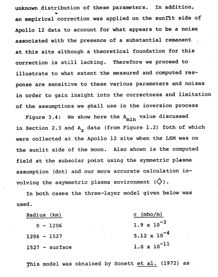
2.3 Data on the A . Values at the Apollo 12 Site 45 2.4 Observation of a Large Interplanetary Magnetic 54

Field Discontinuity

3.1 Numerical Mismatch in the Continuity of H 77 3.2 Numerical Mismatch in the Continuity of He 78 3.3 Numerical Mismatch in the Continuity of H 80

r

3.4 The Computed Response from the Asymmetric and 84 Symmetric Plasma Theory and the Measured A and

Ami_n Data Z

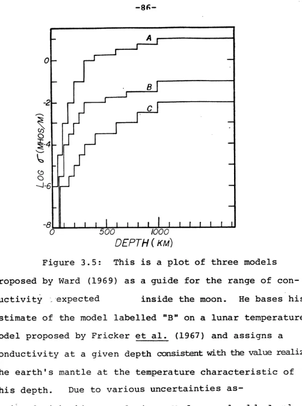
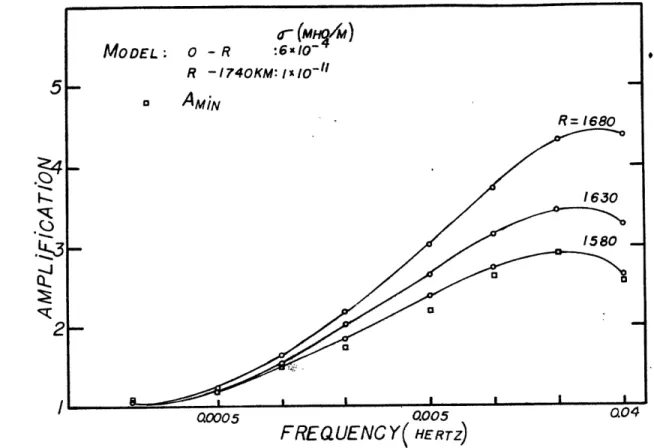
3.5 Three Conductivity Models, A, B, C, Proposed by 86 by Ward

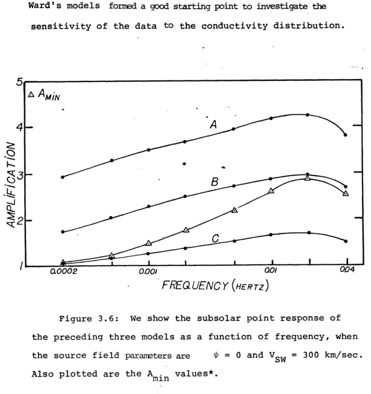
3.6 Subsolar Point Response of Model A, B, and C 87 3.7 Antisolar Point Response of Model A, B, and C 88 3.8 Computed Subsolar Point Response for a Set of 90

Two-Layer Models

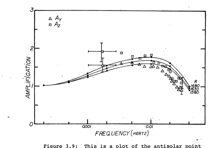
3.9 Computed Antisolar Point Response for a Set of 91 Two Layer Models

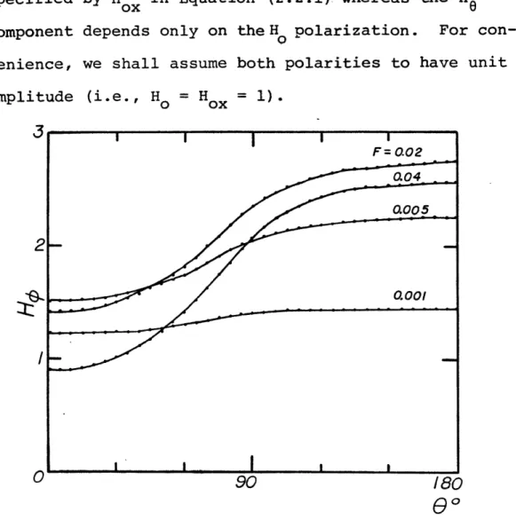
3.10 Plot of IH vs. Polar Angle for a Set of Fre- 94 quencies

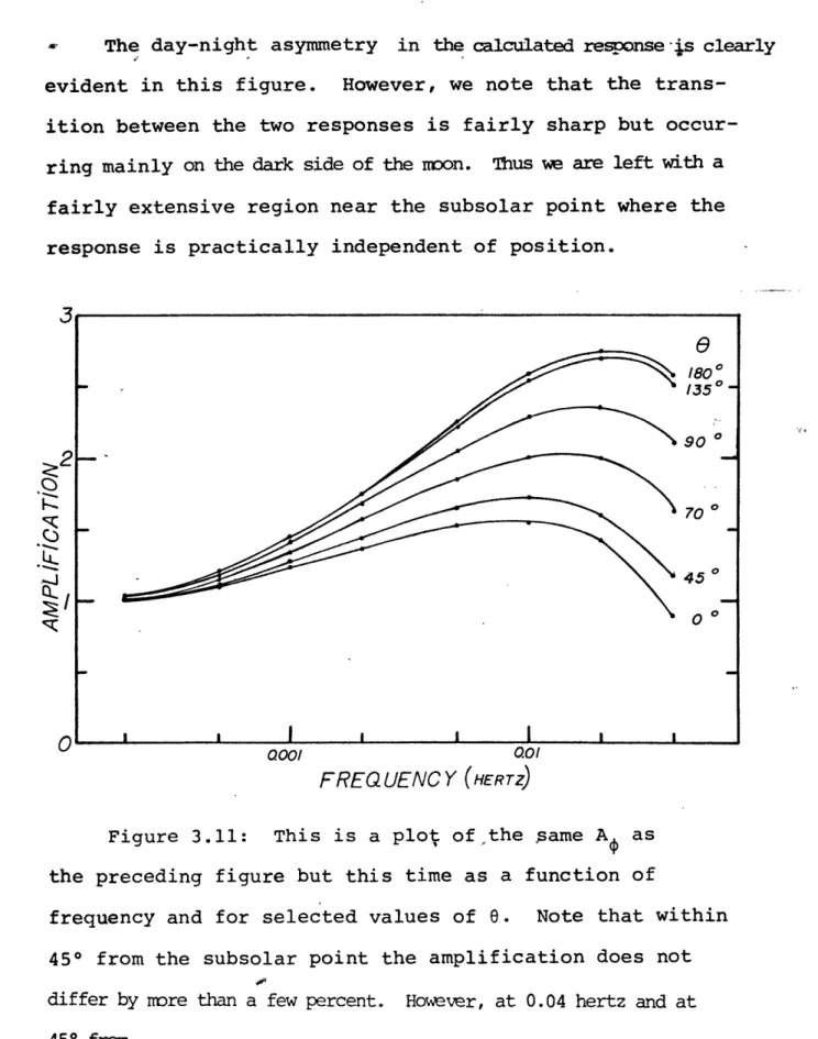
3.11 Plot of A vs. Frequency for-a Set of Polar 95 Angles

3.12 Plot of the Values of A at the Subsolar Point for 96 a Set of the Solar Wind Velocities

3.13 Plot of the Values of A at the Subsolar Point for 97 a Set of Angles of Incidence of the Source Field

3.14 Plot of the Values of A at the Antisolar Point for 98 a Set of Values of the Solar Wind Velocity

3.15 Plot of A at the Antisolar Point for a Set of 99 Angles of Incidence of the Source Field

3.16 Plot of the Absolute Value of H8 vs. Polar Angle 100 for a Set of Frequencies

3.17 Plot of A₈ and A vs. Frequency for a Set of 102 Polar and Azimuthal Angles

3.18 Plot of the Dark Side AR Response vs. the Polar 104 Angles of a Set of Frequencies

3.19 Plot of AR vs. Frequency for a Set of Values for 106 the Solar Wind Velocity

3.20 Plot of AR for a Set of Values of the Angle of 107 Incidence of the Source Field

4.1 Conductivity Model and Parameter Resolution Ob- 121 tained Using V = 200 km/sec and A _{sw mn} data in the Inversion 4.2 Fit to Amin Data and Information Distribution for 123

a Model Obtained Using V = 200 km/sec sw

4.3 Conductivity Model and Parameter Resolution Ob- 125 tained using Vsw = 400 km/sec and Amin Data in

the Inversion

4.4 Fit to the Amin Data and Information Distribution 126 for Model Obtained Using Vsw = 400 km/sec

4.5 _{Conductivity Models Obtained Using a Different 127} Set Layer Thickness in the Inversion

4.6 Conductivity Model and Resolution Obtained 130 Using the Aiin, A. and A, Data in the Inversion

4.7 Fit to the A , A_z and A Data 131

minz y

4.8 Conductivity-temperature Plot Resulting from 136 Inversion and from Laboratory Data

4.9 Lunar Temperatpre Models Proposed by Toks8z et al. 138 4.10 Fit to the A data of Conductivity Models Con- 141

strained by the Low Temperature Model of Toks6z et al. when a Set of Values for Vsw is Used in the Inversion

4.11 Fit to Az and Ay Data and of Conductivity Model 143 Constrained by Low Temperature Model of Toks8z

et al.

4.12 Resolution of Parameter Correction for Models 144 Giving Best Fits to Amin, Ay Az Data

4.13 A Family of Temperature Models ₁₄₇

4.14 Fit to A . _{Data and Model Obtained when the 149}

min

Temperature Model has no Gradient Below 200 km

4.15 Model Obtained Assuming a Water Saturated Moon 152

AP-II Computed Response in the Void to Interplanetary 172 Discontinuity

AP-VI Absolute Value of Partial Field Associated with 190 Each Fourier Harmonic of the Radial Component

of the Magnetic Field vs. Polar Angle, for m = 1-6

Tables _Page 1.1 Remanent Field at Various Apollo Sites 24 3.1 Relative Error in Fitting the Boundary Con- 82

ditions Through the Frequency Range of Interest

3.2 A Conductivity Model Giving a Good Fit to 93 the A . Data

mln

4.1 _{Semiconduction Parameters Resulting from In- 140} version Using the A data and Low Temperature Model of Toksiz et al.

4.2 _{Semiconduction Parameters Resulting from In- 142} version Using A min, A_z and A Data with the

Low Temperature Model of Tokstz et al.

4.3 _{Semiconduction Parameters Obtained Using 146} Ami_n Data and a Family of Temperature Models

AP-V Values of M _m (2p) and N (2p)

Chapter I

Historical Introduction

1.1 Introduction

Two major experiments have been the turning point, in recent years, in our understanding of the moon's electromagnetic environment. On July 22, 1967, the Explorer 35 spacecraft was injected into a stable lunar orbit carrying magnetometers, energetic particle detec-tors, and plasma probes on board. The results of this experiment were to unravel the essential feature of the interaction of the solar wind with the moon. However, it turned out that no effect of the conductive lunar in-terior could be detected at the satellite orbit. Such signals were not conclusively obtained until the deployment of the Apollo 12 lunar surface magnetometer (LSM) on

November 19, 1969. Since the evolution of our concept has been largely shaped by the data obtained in these two ex-periments, they provide a natural division in the short history of the subject.

1.2 The Pre-Explorer 35 Period

In order to develop a quantitative theory of the

interaction of the solar wind with a planet, it is essential to know the magnitude of the steady, global magnetic field this planet might possess. At the earth's orbit, this field needed only to be of the order of 50 gammas in

order to balance the dynamic pressure of the solar wind and thus form a bow shock on the sunlit side of the moon (Willis, 1971).

The results of the early spacecrafts sent to the moon were not entirely conclusive on this question. The

Luna 2 probe (Dolginov, 1961) did not observe any per-turbation of the interplanetary field at 50 km above the sunlit lunar surface, when the moon was in the magneto-sheath. The accuracy of the instrument was about 100 y, so this experiment did put a fairly accurate upper limit on the global magnetic field that might be present on the

lunar surface. However, the possibility that a shock existed was not completely ruled out. A steady dipolar

field of about 50 y presumably would be compressed to within a few plasma skin depths (= 2 km) of the lunar

surface and thus be hardly observable at an altitude of 50 km.

The interaction of the solar wind with an electrically conductive lunar interior might also build up the required 50 y for a shock. Two modes of interaction are possible. In the poloidal H mode, eddy currents are generated in-side the moon by the time-varying interplanetary magnetic field. _{If we consider an homogeneous lunar model, these}

fluctuation to within a skin depth,

2 12

of the lunar surface. Moreover, since the solar wind presumably shields itself from the magnetic field

generated by these currents, through confining current flowing within a few plasma skin depths from the lunar surface, an interplanetary fluctuation associated with a lunar skin depth much smaller than the radius of the moon would be amplified roughly by a factor RM/6 on the lunar surface. If we assume that a shock is produced by the

sector .structure fluctuation of the

interplanetary magnetic field, B 5.y, period = 10 days, (Schatten, 1971), then we require a near surface lunar conductivity higher than a few mhos/m (6 - 0.1 RM).

Such high conductivity, typical of sea water on earth, was considered by Sold (1966) in a qualitative analysis of the interaction of the solar wind with the moon. Tozer et al. (1967) quickly pointed out, however, that if water is not present inside the moon, the bulk lunar conductivity is likely to be determined by the tem-perature and composition at a given depth. Using a

temperature model proposed by Urey (1962) and the con-ductivity-temperature relationship for an olivine with 10% fayalite, they showed that a conductivity of a few mhos/M is likely to be reached only deep inside the moon (R = 800 km). They thus dismissed the possibility

for the poloidal H mode to produce a detached bow shock in front of the moon. However, apparently omitting the possibility for the magnetic field line to slip around the core, Tozer et al. concluded that the field lines will accrete in front of the core and thus produce an attached hydromagnetic

shock near the limb of the optical shadow.

The toroidal H interaction was investigated by Sonett et al. (1967). In the rest frame of the moon, the interplanetary magnetic field, BSW _, is seen to be ac-companied by an electric field given by

S= -Vsw x BSW _(1.2.1)

An exact determination of the solar wind velocity, VSW, involves not only the streaming speed of the

solar wind (= 350 km/sec), but also the various motions of the moon.. However, even the r.mst important of these motions, the rotation around the sun together with the earth

(- 29.8 km/sec), has a magnitude much smaller than the bulk solar wind velocity. Thus these notions will be neglected

Let us approximate the moon by a cylinder with axis parallel to the E field, with radius equal to the moon radius and with length twice this value. The

po-tential across the cylinder is then given by

= 2RME = 2_{RMVSWBSW (1.2.2)}

where we have assumed the solar wind magnetic field to be perpendicular to the solar wind velocity.

Equation (1.2.2) also assumes that the electric con-ductivity of the solar wind is very high so that no electric field is seen in the rest frame of the wind. By Ohm's Law, we have

TRM

I R. - a (1.2.3)

Re 2

where I is the current and Re the resistance along the cylinder axis and a is the cylinder conductivity. From Ampere's Law, and combining.Equations (1.2.2) and (1.2.3) we obtain

iI

Btoroidal =2RM o RM-VSSW (1.2.4)

where for a homogeneous cylinder a = 0.5.

We note that, for field fluctuations associated with an interplanetary wavelength and lunar skin depth much

larger than the radius of the moon, the toroidal H in-duction field is independent of frequency. Moreover, if the conductivity is about 3 x 10-5 ho/m, the toroidal H field at the lunar surface is nearly ten times the solar wind magnetic field. In that case, a shock might be

formed on the sunlit side of the moon. However, even if the interior conductivity of the moon is higher than 10-5iho/m but is covered by an insulating layer, the toroidal H field may become much smaller than the solar wind field. Let us assume our cylinder to be capped by

layers of thicknesses A and neglect the internal

re-sistance compared to the one at the surface (the rere-sistance to the current flow added in series). Then, the toroidal H field is still given approximately by Equation (1.2.4) but with a = 0.5 R/A and a equal to the crustal

conduc-tivity. A 17 km crust with conductivity 3 x 10- 7 _mho/m still gives a surface field ten times higher than the solar wind field. However, if the conductivity-thickness ratio of the surface layer is a hundred times smaller

-8

than 2 x 10 mho/m-km, then the toroidal H field becomes only one tenth of the solar wind field, at the surface of the moon.

In situ, measurement of rock conductivity at the sur-face of the earth has not revealed conductivity much

-5

lower than 10- 5 mho/m. But this is due mainly to the presence of water in the earth crust (Madden, 1971, and Brace, 1971). Laboratory measurement on dry rocks have shown, however, that conductivity lower than 10- 8 mho/m can easily be reached at room temperature (see, for ex-ample, Fensler, 1962). Because of the relatively large range of conductivity one might assume for the surface of a planet, predicting the importance of the toroidal H mode will probably remain difficult.

During a month in 1966, the Luna 10 spacecraft

was placed in lunar orbit and sent back to earth additional data on the magnetic field around the moon. A very regular

field of 23 to 40 y was observed (Dolginov et al. 1966). This field did not vary much either along an orbit of the satellite around the moon (periselene: 1.2 RM; aposelene: 1.7 RM) or along the orbit of the moon around the earth. Though the regular behavior of the field rendered the measurement somewhat suspect, Dolginov et al. (1967) pro-posed a possible interpretation in terms of the inter-action of the solar wind with a conductive lunar interior.

1.3 From Explorer 35 to Apollo 12

Explorer 35 has a stable orbit of period 11.5 hours, aposelene = 5.4 RM , and periselene = 1.4 RM . The

(Ness et al., 1967, and Lyon et al., 1967) were to be confirmed by subsequent instruments sent to the moon.

Contrary to what was observed by Luna 10, no

steady lunar magnetic field, of magnitude several times the average solar wind field, was found. Behannon (1968) by examining the Explorer 35 data, obtained when the moon traversed the neutral sheet of the geomagnetic tail, was able to distinguish the magnetic field of a possible per-manent lunar dipole from the one induced by a bulk lunar permeability. He was thus able to establish an upper limit of 4 y on the permanent dipole field at the lunar surface and an upper limit of 1.8 for the bulk relative magnetic permeability of the moon.

No bow shock wave was observed. As we have seen

above, a possible explanation for the absence of a toroid-al H mode-induced shock is the presence of a surface layer of conductivity thickness ratio smaller than

-8

2 x 10 mho/m - km. The fact that the time variation of the interplanetary magnetic field associated with its sector structure does not produce a poloidal H type of shock tends to imply that the conductivity in the top 200 km of the moon is smaller than a few mhos/m.

When the moon is in the solar wind and the satel-lite passes through a cylinder approximately defined by the optical shadow, several effects of the interaction of

the solar wind with the moon were observed. The plasma flux (50 < Ep< 2850 ev) decreased by several orders of magnitude consistent with the hypothesis that the particles in the solar wind were absorbed on the sunlit surface of the moon, leaving a void on its downstream side. The magnetic field was also perturbed (Figure 1.1). Near the boundary of the optical shadow a small decrease in the field magnitude is'followed by a gradual increase in the plasma umbra (Colburn et al., 1967, and Taylor et al., 1968). Several theoretical attempts were made to explain these characteristics. Spreiter et al., (1970), using the

equations of magnetohydrodynamics, examined the case where the interplanetary magnetic field is aligned with the

flow direction. This particular field configuration was reported by Ness et al. (1968), and their results agree qualitatively with the observations. They found that the

small decrease can be understood in terms of the approximate conservation of the ratio of magnetic field to particle

density along a streamline. The solar wind particles initially tend to fill the void thus decreasing particle density, pressure and magnetic field along a streamline. These gradients are accompanied by current that increases the field of the plasma umbra. An equilibrium void/plasma boundary is reached when the umbral magnetic pressure

balances the particle and magnetic pressure of the solar wind.. Whang (1970), noting that the scale length

as-sociated with the observed field gradient is generally larger than the proton gyroradius (= 100 km), used the guiding center approximation to calculate the field and

particle distribution. His treatment included the effect of anisotropic propagation of the magnetosonic wave in addition to the more general field configuration.

Y i NESS.BEHANNON.TAYLOR,& WHANG + I-zi 0 SISCOECLYON,ISACK.S BRIDGE . + SHADOW + 2100 2130 2200 2230 U.T. EXPLORER 35 5 AUGUST 1967 Figure 1. 1

Simultaneous measurements of field and

plasma obtained on August 5, 1967, from lunar orbit on the Explorer-35 spacecraft. The trajectory of the spacecraft is shown projected on the ecliptic plane and positionally correlated with the data through UT annota-tion. The x axis is parallel to the sun-moon line.

A fundamental aspect of the interaction is the fact that the Alfven and sound speed (= 30 km/sec) are much lower than the bulk solar wind velocity. Consequently, a given position in the solar wind, on the downstream side of the moon, will be influenced by the disturbed

con-dition at the plasma-vacuum boundary only if it is

within the Mach forecones originating at the terminator (the limb for solar wind flow). The existence of such Mach cone received sqme experimental support by Whang et al. (1970). Also, Ogilvie et al. (1970) showed that the amplitude of the umbral increase and penumbral de-crease tend to grow in proportion to the ratio of par-ticle to magnetic pressure. However, since, to date, only a subset of the parameter that influences the field charac-teristics have been compared to the theory, its detail-ed confirmation must still be considerdetail-ed incomplete.

In addition to the two characteristics just men-tioned, a small increase of the magnetic field was often observed on the interplanetary side of the penumbral decrease. This feature was shown to correlate with a

small enhancement in particle density (Figure 1.1). (See Siscoe, 1969). Hollweg (1968) suggested that if

toroidal H field, might be induced. The interaction of the solar wind with this field would presumably produce the small external increase. However, chemical analysis of lunar samples brought back to earth in the Apollo 11 mis-sion did not show any evidence of hydrous phases in lunar rocks (see, for example, Charles et al., 1971). Schwartz

et al., (1969), pointed out, though, that a dry moon, with a hot interior, might also produce a significant toroidal H field, depending on its near-surface conductivity. But Ness (1972), in a review of the subject, argued against

this possibility on the basis that the small peak is often observed when the interplanetary magnetic field is aligned with the solar wind flow velocity. According to

Equation (1.2.1), no motional electric field should exist in that case.

In view of the absence of bow shock and in

anticipation of the lunar surface magnetometer experiment, the response of the moon to time varying magnetic

fluc-tuation was also re-evaluated theoretically by several workers (Blank et al., 1969, Schubert et al., 1969,

Schwartz et al., 1960, Sill et al., 1970). They showed that the expected frequency dependence of the poloidal H * lunar response might enable us to distinguish between

several possible lunar conductivity profiles, in particular between a hot and cold moon based on the conductivity

The concept that the solar wind interaction with the moon does not perturb regions outside the Mach cones on the downstream side of the moon was found to break down for frequencies higher than approximately 0.1 Hz (Ness et al., 1969). High frequency fluctuations seemed to originate at the plasma vacuum interface and to propagate,

outside the plasma umlbra, along the time average magnetic field lines threading the lunar wake. A higher level in the power spectral density above about 0.1 Hz was seen to be maintained-in a region within approximately one lunar radius of the plasma/void interface. A tentative explanation for this phenomenon was given by Krall et al.

(1968) in terms of an electron ballistic effect. They argue that the solar wind electrons (thermal-speed

= 2000 km/sec, gyroradius = 2 km), upon reflection at the

solar wind/void interface, will carry a memory of the perturbed condition at this boundary. This memory, which manifests itself as a fluctuating magnetic field

as-sociated with current produced by a perturbation of the electron distribution function, will eventually fade away by phase mixing as the electrons travel away from the boundary.

1.4 From Apollo 12 to Recent Years

Several magnetometers were flown to the moon during the Apollo missions. One highlight of these experiments was

the discovery of local reanent magnetic fields at most

Apollo sites (see Table 1.1 from Dyal et al., 1972, 1973 a, b). Table 1.1 Site Location Apollo 12 Apollo 14 Apollo 15 Apollo 16 Oceanus Procellarum (3.20S 23.40o) Fra Mauro (3.7oS 17.5OS) (two sites 1.1 km apart) Hadly-Apennines (26.1oN 3.7E) Descartes (8.90o 15.50 E)

(five sites separated by 0.5 to 7.1 km) Steady Magnetic Field (7) 38±3 103±5 43±6 6±4 327 232 189 113 113

In addition to these instruments, two subsatellites, with magnetometers on board, were launched during the Apollo 15 and 16 missions along orbit near the surface of the moon (= 100 km). Data from these subsatellites were used to map the lunar remanent field (Coleman et al.,

1972) and also to place an upper limit of 3.6 x 1018 gauss-cm3 _{on the permanent magnetic dipole moment of the moon}

mag-netic moment is at most 4.5 x~10- 8 times as strong as the one of the earth and can only produce a surface field smaller than 0.2 y. A review of the magnetic proper-ties of lunar rocks can be found in Fuller (1974).

New bounds on the bulk relative magnetic permeabi-lity of the moon (U- = 1.03-0.02) were established by Parkin et al. (1973) by considering the data from

Explorer 35 and the lunar surface magnetometers when the moon was in the geomagnetic tail.

No significant toroidal H field was found on the surface of the moon. However, the discovery of a large

remanent magnetic field leads to the suggestion by Barnes et al. (1971) that when such a field is present near the

terminator, it might interact with the solar wind to produce the observed small limb compression. A

prelim-inary check of this hypothesis was made by Lichtenstein et al. (1974) with the data from the Apollo 15 subsatel-lite. They found that the occurrence rates of limb com-pression are roughly proportional to the amplitudes of the renanent fields observed at satellite altitude.

Large amplification of the tangential components of the magnetic field at the lunar surface was observed by comparing the magnetic fluctuations at Explorer 35 to

the one at a LSM when both instruments were on the sunlit side of the moon and outside the geomagnetic tail (see,

for example, Sonett et al.,1971 a). Detailed power spectral density of each component of the field was evaluated at the

L L

LSM (PLSM) and Explorer 35 (PE) when the latter instru-ment was on the upstream side of the moon. If, at an LSM site, we define a mutually orthogonal set of unit vectors x, y, z (vertical, eastward and northward, respectively), then the data can be expressed in the form of an ampli-fication factor AL (L = x, y, z) were

L L 1/2

AL = (PLSM/PEXP

The coordinate system used to evaluate the power spectral density from Explorer 35 is made to correspond to the one used at the LSM site. The data is presented in Figures 1.2, 1.3, and 1.4. These power spectra were evaluated when the moon was either in the free streaming

solar wind or in the earth's magnetosheath. Figure 1.2 represents data obtained at the Apollo 12 site when the LSM was on the sunlit side of the moon. The data in

Figure 1.3 were also obtained at the Apollo 12 site but the LSM was on the night side of the moon, within 450 from

the antisolar point. Figure 1.4 represents data ob-tained at the Apollo 15 site when the LSM was on the

O-P

IMI8c

_oo6o

(>0orpp

B

_oa~

d

OOooQD

vl

f

0-fI

e

B[3E

10-2

FREQUENCY,

HZ

1.

<[

_w

H

z

IC/)

z

1-3

10-4

_4x10"2

I

II

I

ooooop

888888

.

Ax

a

2~

,

.1.

O.

.I

I

I

0.0005

0.00

1

0.002

002

0.5

0.0

0.02

0.04

FREQUENCY

(HERTZ)

SA

z

SAy

O

_Ax

_zA

_A

Qo01

FREG

UENC

Y

Z

t-e

~Ci[:

L,

sJ

rC

IH

-00

0.01

(HERTZ)

-sunlit side of the moon, within 450 from the terminator. The data in Figures 1.2 and 1.3 are from Smith et al.

(1973), whereas those in Figure 1.4 are from Schubert et al. (1973). The technique used to evaluate these

spectra has been discussed by Sonett et al. (1971 b). Recently, Schubert et al. (1974 b) have published the amplification factors obtained when the moon was in the plasma sheet of the geomagnetic tail. These latter data will not be used in this thesis.

In the initial inversion of the sunlit side data, Sonett et al. (1971 c) assume the solar wind plasma to be radially incident on the moon. They obtain a conduc-tivity profile characterized by a relatively large spike at a depth of approximately 250 km. But conductivity

pro-files with this peaked behavior were soon recognized to be only part of a larger set of models, many of which

smoothly varying, that fit equally well the frontside data. (See, for example, Kuckes, 1971 and Sonett, 1972.)

The night side data were initially interpreted by Dyal et al. (1973b ), who investigated the passage of

large magnetic field discontinuities in the solar wind. They assumed the moon to be surrounded by a vacuum and inverted the time domain response of the moon to these

discontinuities. They found that, in addition to a constant conductivity layer of 3 x 10- 4 mho/m in the upper 700 km of the moon (except for a thin --

=

order to fit the decay time of the vertical magnetic field component of the discontinuity. Schubert et al. (1973 a), however, showed that, using the vacuum approximation, the radial amplification factor in Figure 3 poorly resolves the conductivity of the bottom layer. Moreover, they showed that the tangential amplification factors on the

night side cannot be inverted within a model that assumed the moon to be embedded in a vacuum. This is due to the neglect of confining current on the frontside of the moon and at the plasma vacuum boundary. The effect of these currents is to amplify the tangential surface magnetic

field to a value higher than can possibly be reached by any conductivity model within the vacuum approximation.

The radially incident plasma model also suffers from its neglect of the plasma void. behind the moon. One aim of this study is to incorporate in a single model the dayside-nightside asymmetry in the plasma environment of

the moon. Concurrent with our effort, Schubert et al. (1973, b, c), Schwartz et al. (1973) and Smith et al.

(1973) have recently published initial results of a theory which account for the day-nightside asymmetry. We shall discuss some of their results as we go along in the next chapters.

1.5 Thesis Outline

Chapter II contains the field solution in the

different regions around the moon, together with a dis-cussion of the boundary conditions used in the analysis.

In Chapter III we discuss the numerical method used to solve the forward problem together with the properties of the solution for various lunar conductivity models and

solar wind parameters.

In Chapter IV we solve the inverse problem for particular sets of parameters of the source field and discuss the resolvable feature of the conductivity structure together with the information distribution among the observations. Also, we subject the moon to

various temperature models and discuss inferences that can be made on the parameters of a semi-conductor satisfying both the thermal and magnetic constraints.

2.1 Introduction

We will consider only the period of the lunar month when the moon is either in the earth's magnetosheath or in the free streaming solar wind. During this period we can distinguish three regions in the moon's electro-magnetic environment: the solar wind, the void

cavity behind the moon, and the interior of the moon. In the following sections we discuss the field repre-sentation in each of these regions and their coupling through the boundary conditions.

The different coordinate systems used to represent the field are shown in Figure 2.1. Their origins should all coincide with the center of the moon but for clarity they have been translated parallel to the solar wind velocity. We will follow Morse et al. (1953) for the definition and notation of the various functions used

in the text.

Since we expect the lunar response to be somewhere between the one expected for a spherically symmetric plasma and a vacuum environment, it is instructive to compare

some of their characteristics before attempting to in-corporate the various regions around the moon into a

Figure 2.1

more comprehensive-model. This is especiallyigtrue in our case since the solution of the more realistic model can be reached only through a numerical method which lacks, to some extent, the insight provided by a simple close-form formula.

To avoid any of the complications arising from the structure, of the source field, we shall assume the inci-dent field to be spacially homogeneous and given (see Figure 2.1) by:

+inc + + +

H = Ha = H (a sinOsin+ cosesin +a cosf) (2.1.1) In the vacuum approximation, we allow the

induced field to expand into a void outside the moon We can express the total field in the void as the sum of the in-cident field and the field of a dipole, i.e. :

-vac -+inc RM

H = H + VxVx b r sinesina (2.1.2)

r r

where r is the distance to the center of the moon and b is a constant to be determined by the boundary con-dition.

In order to gain some insight into the amplitude of the response, let us assume that the moon is formed of two layers, the top one an insulator and the bottom one a perfect conductor. The field in the insulating

shell is given by

oon = V x V x (c _r + dr2) sinOsina (2.1.3) r

In both models, the magnetic field inside the moon must have a vanishing normal component at the surface of the perfect conductor of radius a. In the vacuum ap-proximation, the three components of the magnetic field must be continuous at the lunar surface. In the sym-metric plasma assumption, however, since we assume the induced field to be confined by a thin current layer above the surface of the moon, it is only necessary to equate, at the lunar surface, the normal component of the magnetic field inside the moon to the one of the incident

field, as given in Equation (2.1.1). If we apply these boundary conditions and extract from the result the ratio of the tangential component of the magnetic field at the lunar surface to the one contained in the incident field, we obtain 3 Avac 1 + a (2.1.4) 3 2RM 3 3 Ap l _{asma = 1 + a(2.1.5)} 3 3 R - a

These responses are plotted in Figure 2.2. We note first that the -' uum response can only reach an upper

O.2

0.4

0.6

R/RM

Figure 2.2

limit of 1.5. Since the data of Figure 1.3 exhibits

measured value higher than this when the LSM is near the antisolar point, one can readily infer that the vacuum approximation is inadequate to interpret the tangential amplification factor in the more realistic geometry. Another point of interest is the detectability of con-ductivity deep in the lunar interior. For example, if we assume the data to have a 10% relative error due to noise, we note that even a perfect conductor of radius

lying between about 700 km (a = 0. 4RM) and 1000 km (a = 0.6 RM), would yield a response only of the order of the uncertainties in the data.

A similar treatment can be given for the toroidal H magnetic field but since these results are completely

worked out in Sill (1970) and are similar to our deriva-tion in a simpler geometry given in Secderiva-tion 1.2, we

omit them here and proceed directly to the task of representing the field in the various regions of the lunar environment.

2.2 Representation of the Field in the Solar Wind In addition to its quasi-stationary sector

structure, the interplanetary magnetic field is usually permeated by various magnetohydrodynamic shocks, dis-continuities and waves. (For a review of the first two types of disturbance, see Burlaga, 1972). Belcher et al. (1971) have found substantial evidence that the

power spectral density of the interplanetary magnetic field, in the frequency range where lunar induction has been measured (Figure 1.2), is dominated at least

fifty percent of the time by large amplitude Alfven waves, propagating outward from the sun. Sari et al.

(1969) have proposed an alternative model to explain

these micro-scale (< 0.01 au) fluctuations. They suggest that the interplanetary magnetic field has a spaghetti-like filamentary structure, with bundles of lines-of-force separated from one another by tangential discon-tinuities and essentially static in the rest frame of the solar wind. Though the physics involved in these two models differs markedly, these differences are of little consequence for our application. A common charac-'tristic that must be retained, however, is that the

inter-planetary magnetic fluctuations, as seen in the rest

frame of the moon, are essentially convected at the solar wind speed. This approximation seems appropriate for the free streaming solar wind but the increase in the plasma pressure in the magnetosheath might produce wave velo-cities which are a substantial fraction of the solar wind velocity. Unfortunately, the data presented in Chapter I did not differentiate between these two lunar environments, so some caution should be used in their

interpretation. We should note here that for

waves propagating nearly perpendicular to the solar wind velocity, their phase velocity plays an important role in determining their spatial structure. Since such waves probably represent only a small fraction of the power density spectrum of the fluctuation, their con-tribution to the response shall not be considered any further.

We shall assume that we can represent the fluctuation as a superposition of plane waves convected as a constant solar wind velocity, VSW. In the first of these hypotheses, we assume that the magnetic fluctuations are not generated near the moon and thus have little sphericity in their structures. _{In the second assumption we ignore perturbation} such as large solar-flare-associated

shocks which significantly modify the solar wind velocity A change of 100 km/sec in the bulk speed within a

minute's interval can occur during such events (Chao, 1970).

Let us choose the y-axis in Figure 2.1 such that the wave normal to a given fluctuation is in the y-z

plane and subtends an angle ip _{with respect to the solar wind velocity.} If we assume 4 to be positive if the wave normal has a

field as follows.*

=H _O (aO4-a in) ei k _{(zcos +ysin*)} H= 0(a cos*-asinp)e +H 4 eik (z cosW+ysin*) * ox x where kcos* - k = (2.2.1) ksing E k L VSW tan*

SW

A time factor, e-i t, is implicitly used here, as in all similar equations of this chapter, and w

stands for the angular frequency measured in the rest

frame of the moon. In the solar wind rest frame, however, a fluctuation with phase speed Vph and propagating paral-lel to the solar wind velocity is seen with an angular

wVph frequency equal toV

VSW +Vph

For example, an Alfven wave, at the highest angular frequency for which the lunar response has been measured, 0.25 rad./sec. (Figure 1.2), has an angular frequency of 0.02 - 0.05 rad./sec. in the solar wind frame. This is still about an order of magnitude smaller than the nominal

proton gyrofrequency in the solar wind (0.5 rad./sec). Also for the case of an Alfven wave, we have neglected the

electric field in the rest frame of the wind. Equation (2.2.1) should still give a good first order approximation, however, since this electric field is smaller than the one associ-ated with the motion of the solar wind by the factor:

Vsw

-- = _{(5 - 10).}

A

2.3 The Field Inside the Moon

We assume the moon to consist of spherical layers of constant thicknesses and homogeneous conductivities. Such a structure is in harmony with a lunar model where the conductivity is mainly determined by the composition and temperature and where both can be assumed to vary only along the radius. If thermal conduction is the main heat transfer process inside the moon, this would seem to be a reasonable assumption for the temperature distribution. However, if solid state convection plays an important role in heat transfer, Turcotte et al.

(1972) have suggested that a significant asymmetry in the temperature distribution could be introduced at depth where convection occurs.

Also, if extensive lateral inhomogeneities in a global radially-varying moon structure are located near a given magnetometer, they might significantly influence

the signal observed at this instrument, especially at the higher frequencies. Even though power spectral data have been published from only the Apollo 12 and 15 site

magnetometers, already there is substantial evidence that a regional signature is detected at the latter site. Schubert et al. (1974c), by examining the power density spectrum at different angles in a plane tangent

to the surface at the Apollo 15 site, found that the distribution of power is strongly peaked along the northwest-southeast line

at frequencies above approximately 5 mHz. This

direction of polarization seems to be observed consistently and is independent of the directional character of

the solar wind power spectrum and of the position of the magnetometer in the asymmetric plasma environment. A likely expalantion for the anisotropic character of the response is that some regional inhomogeneities influence the data at

the site. Maxima in the power spectrum of the tangential magnetic field components were also observed at the Apollo 12 site. But since between approximately 0.001 and 0.02 Hz, the peak tends to

align along a line parallel to the tangential component of the remanent field at this site (= 640 south of east), it was tentatively attributed to a modulation of this

field by fluctuations in the dynamic pressure of the solar wind (Sonett et al., 1972). We examine briefly

out here that anisotropy in the power spectrum of the tangential magnetic field component is also observed by the Apollo 12 magnetometer when this instrument is on the dark hemisphere of the moon. Its detailed pro-perties have not yet been presented in the literature, but its existence can be inferred from Figure 1.4. So a regional influence on the data might also accompany the noise due to the remanent field at this site.

Thus, even if the bulk of the moon can be model-

-led approximately by a radially-varying structure, we never-theless face the problem.of extracting its global

in-duction signal from data contaminated by noise and regional inhomogeneities. A first empirical step in

that direction was made by Sonett et al. (1972) who estimated the values of the tangential amplification factor at the Apollo 12 site, along a direction such that this quantity is minimal (e.g., between 0.001

and 0.02, along a line parallel to -E250N, i.e., ortho-gonal to the direction of the tangential remanent field). We show these data, Amin, in Figure 2.3, together with the data of Figure 1.4 (and a data point from Figure 1.2). We note that the Apollo 15 data, though probably

northwest-APOLLO

*

_AMIN

OAy

12

APOLLO

oAy

SAz

15

.p

SI

0.002

0.005

0.01

0.02

FREQ.UENC

Y(

0

Q,

0.0002

0.0005

0.001

HERTZ)

0.04

southeast line, agree fairly well with these Ami_n values. This set of data thus probably represents a good first approximation of the global response of the moon. But, of course, in order to qualify this

in-ference, a more detailed data analysis is required, in conjunction with theories that account for the possible

regional influences and other sources of noise. We now turn to the solution of the

Maxwell equation inside a layered sphere. These solutions are well knan so we shall only summarize

some of the main results here.

The continuity of the tangential components of the A and A fields* can be applied to each of the two electro-magnetic modes independently at an internal boundary of the sphere. This permits us to determine, for each har-monic of each mode, the ratio of electric to magnetic field at the lunar surface. Instead of dealing with im-pedances, however, we found it convenient to define, in

Appendix II, some related quantities, Ln and Tn, which per-mit us to write the field as follows:

Here we assume the moon to have a constant permeability equal to the free space value.

sin aH E a n(n+l) a m (cosa) { } m a nm n cos n,m Pm (cosO) sin + [amLn { }m nm n a6 Cos

mba T P (cose) cos + ik //R sin8 sin

Pm (cose) cos

[ma L n }m9

a [ nm n sine sin bnmTaPnm (cosa) sin

ik/ RMe cos

and V

Sn(n+)b_{o SW r nm} o n _{2 n} pm (cose) sinm _cos (2.3.1)

nm _(kRM)

n n Cos

Sa [+mik//RManm sine sin} m

am (cos) a ban sin nm 39 Cos b pn (cos ) + C. n sin + a [-anmi k/ / n m n s m

Pm(cosa)

where k2 = iwoOs (as is the conductivity of the sur-face layer) and k is defined in Equation (2.2.1).

:The coefficients a and b are the coefficients

nm nm

of the poloidal and toroidal H mode, respectively, and are to be determined by applying the boundary conditions at the lunar surface.

2.4 The Field in the Void Region on the Downstream Side of the Moon

In order to obtain a tractable representation of the field in the void region on the dark side of the moon, some assumptions must be made on the parameters of the solar wind. We shall adopt the following three hypotheses:

1. We can treat the solar wind as a cold plasma. In other words, we shall neglect any effect of the ther-mal pressure compared to the magnetic pressure.

2. We assume that the ratio of the solar wind bulk speed to hydromagnetic wave speed can be consider-ed infinite.

3. We assume the solar wind velocity to be time-and space-independent both in magnitude time-and direction.

We hasten to point out, however, that the solar wind 8 _{is on average equal to about 1, and finite}

8 effects are readily. observable in terms of penumbral decrease and umbral increase of the magnetic field (Ogil-vie et al., 1969). Moreover, a finite, but high, Mach

number effect has been observed by Whang et al. (1970), who measured a Mach cone angle of 80. But, unfortunately, it is difficult to relax these assumptions or to calculate their probable influence on the data, in the frequency range where lunar induction is important, since (i) simul-taneous data of all relevant solar wind parameters are generally not available, and (ii) we lack a proper theory that accounts for these effects. (To date, even steady state theory predicts some parameter dependence of the magnetic field that has no counterpart in the observation

(see, for example, Ogilvie et al.,1969).

We shall content ourselves in this thesis to check that a theory that incorporates these assumptions does in fact reproduce some of the major frequency-dependent characteristics of the field observed around the moon. This procedure is somewhat unsatisfactory, however, since the agreement comes largely as the result of a

success-ful search for a conductivity profile that satisfies the observations within the framework of the approximation theory. But the very fact that such a model can be

found that agrees reasonably well with both front and backside data, does give some measure of confidence in the approximation theory used. This trust is further improved by the fact that the theory can reproduce at this stage, at least qualitatively, some of the major

frequency characteristics of the field observed in the void region, sufficiently far downstream so that it is uninfluenced by the moon.

In order to discuss this last point, let us ex-amine some of the consequences of the hypothesis we made.

First, the geometry of the vacuum region can

be modelled by a semi-infinite circular cylinder with its radius equal to the lunar radius. Moreover, the

boundary conditions on the electromagnetic field can be most easily obtained since the boundary layer between the void and the undisturbed solar wind can be considered infinitesimally thin. This permits us to match, at the

boundary of the cylinder, the normal component of the solar wind magnetic field and its wavelength parallel to the axis of the cylinder to a solution of Maxwell's equations inside the void. This solution can be given

in terms of a cylindrical TE mode that also satisfies the continuity of the tangential electric field components

across the plasma-vacuum boundary layer. The normal com-ponent of H of the solar wind field, at the boundary of the cylinder, can be evaluated from Equation (2.2.1) and the resulting field inside the void can be expressed as follows:

V o -H = E=E V xm a m,a where a a m = gm I (k /p) 1 of e j 1 o _{e ih} gm* = Y fm + Ym m 2 e hm

gm

E= Neuman factor = 1 when m = 0 and = 2 when m > 0

and where here and in the following development, we use the following definition :

f =

m

h -m

o = 1 _{if m + n + i +} .. is odd mni.. = 0 if m + n + i + ... is even and Ye _{= 0 if m + n + i + ...} is odd = 1 if m + n + i + ... is even

The prime stand for the derivative with respect to the argument and Jm' Im are the Bessel and hyperbolic Bessel functions in their usual notation.

This field is not sufficient, however, to match the boundary conditions on the surface of the moon. To accomplish this, we must add an "end effect field" that will be discussed shortly. But before doing this, let us digress a little to examine some of the properties of Equation (2.4.1).

We note first that for very low frequencies, k//RM << 1, the field is homogeneous and has the same

value as the unperturbed solar wind field. Thus, due to our idealization of the plasma parameters, we do not reproduce the penumbral decrease nor umbral decrease observed behind the moon (Figure 1.1). On the other

hand, for frequencies such that k/M >> 1, Equation (2.4.1)

shows that the power spectral density in the void should be at a much lower level than what is observed in the

unperturbed solar wind. The ratio of the power spectral densit±es in that frequency range and on the axis of the-cylinder, is approximately given by e2 This charac-teristic of the field inside the void is due to the sur-face wave nature of the TE mode. The solution of the vector Laplace equation, propagating along the axis of the cylinder, decays approximately exponentially away from the boundary of the cylinder when kRM>>l. In

harmony with this result, a sharp drop in the power spec-tral density of the magnetic field in the void was observed by Ness et al. (1969), at frequencies above about 0.1 Hz

(k//RM = 3). But a detailed quantitative comparison is hindered by our lack of knowledge of the exact position of the satellite (in particular its distance from the axis of the cylinder) during these observations.

Another type of observation that incorporates both of these limiting features is the response of the void cavity to large discontinuities in the interplanetary

magnetic field. One such event, recorded when Explorer 35 was.near the axis of the cylinder, is shown in Figure 2.4*.

The data in Figure 2.4 and the calculation in Figure AP-III are presented in a right-handed geocentric solar ecliptic coordinate system with +X toward the sun and +Z toward the ecliptic north.

-4 I . . . +4 +2 01 -2 1 : -,- IZI

I

The identical transient at Explorer 33 and 35 using the GSFC magnetometer (5-Hz bandwidth).

SATELLITES LOCATION

IN GEOCENTRIC SOLAR ECLIPTIC COORDINATE SYSTEM

UNIT: EARTH RADII 1 R,

EXPLORER 33 X 37.2 Y -56.3 -23.3 -23.3 EXPLORER 35 59.5 - 8.4 - 4.1 With Respect to the Center of the Moon:

UNIT: _{1 RM}

EXPLORER 35 -1.71 - 0.04 0.26

Figure 2.4

I.

i

-PI'-

Also shown is the observation of the same event by Ex-plorer 33 about fifteen minutes later, while this

satellite, orbiting around the earth, was outside the bow shock.

The difference in the jump in the Z components probably arises due to the finite 8 of the solar wind. Aninterpretation of the other two characteristic

differences, namely the dilatation in the rise time of the Z crponent and the small peak in the X component, in terms of a signature of a conductive lunar interior was

ruled out by Sonett et al. (1971d). Instead they sug-gested that since the two satellites are widely separated

(= 53 RE), the signal difference might be attributed to

a natural difference in the solar wind field at their

locations. Though such solar wind field differences might exist, we examine the possibility in Appendix III that these

characteristics are caused by the surface wave nature of the field in the void region. We find good qualitative agreement with the data using values predicted by

Equa-tion (2.4.1).

We now return to our derivation of the field and proceed to complete our representation by discussing the

At the vacuum plasma interface, the field must have a vanishing normal component of its magnetic field and tangential component of its electric field. This comes about because we assume the solar wind to be unperturbed outside an infinitesimally thin boundary layer at the cylinder boundary. The void region is thus similar to a hollow pipe with perfectly conducting wall. A possible solution of the Maxwell equations in that geometry can be given

in terms of the cylindrical waveguide modes (see, for example, Stratton, 1941). That is:

+ V xE iw'o H a E = . V x a + VxV x D a Z Z 1,mo im zm where ma a 0 /RM sin

2 m A m i oJm( kmP/RM)e {cos }m

(2.4.2)

S= B TJ m (a p/R)e m 3 { _{cosCm Om} }Rsinm

where 8£m and atm' X = 1i, 2,... are the roots of Jm(z) and Jm(z) respectively and where A and B

are the coefficients of the cylindrical TE and TM modes respectively.

Equation (2.4.2) is valid when the frequency is well below the cut-off frequency for mode propagation.

.The smallest cut-off frequency for either the TE or

cB

TM modes is 2 1 = 50 Hz, where c is the speed of

light. Since we are interested in frequencies much lower than this, the approximation is justified.

he mode representation given by Equation (2.4.2) should be sufficiently accurate downstream of the antisolar point but extension of its validity to the lunar surface involves the

so-called Rayleigh hypothesis (Millar, 1973). Indeed, in the vacuum region bounded by the lunar surface and a plane perpendi-cular to the axis of the cylinder and containing the antisolar point there is no physical reason to impose the condition that the modes are decaying downstream. To illustrate this point, let us assume there is a magnetic dipole on the axis of the cylinder half-way

between the center of the moon and the antisolar point. Furthermore, let us assume that the sphere is inside an infinite cylinder. Solution of this problem involves the Green function associated with a magnetic dipole

inside a cylinder (see, for example, Smythe, 1968). This Green function is expressed in cylindrical TE and TM

modes that are decaying upstream for z < RM/2 and down-stre, a for z > RM/ 2 . Though, in that case, the field can be represented by both upstream and downstream decaying modes it does not necessarily follow that in the region z > 0 and (z 2 ₊₂ /_{/2 > we cannot} ex-press the field with only modes decaying downstream. Indeed, this is usually not the case. We recall that the poten-tial field outside a sphere of radius RM_, caused by a

distribution of charge and currents inside it can always be represented by a series of electric and magnetic

multipoles situated at its center. For example, for

the problem above, we can find an equivalent distribution of magnetic multipoles at the center of the sphere, and then use the Green function associated with each multi-pole to represent the total field outside the sphere. Since the equivalent multipoles are situated at the center of the sphere, only +z decaying modes are re-quired in z > 0; but, on the other hand, the expression is valid in general only in (z2 + p2)1/2 > RM.

Let us formalize this concept for the case of the moon. We assume that the field in the downstream cylinder caused by the currents and charges inside the moon and on its sunlit surface can be represented by a series of electric and magnetic multipoles situated at its center. This partial field is the elemenitary solution of Max-well's equations and can be found in most text books

on electromagnetic theory. To the field of each multipole we can add a series of spherical TE and TM modes, regular

at the origin and such that the total field at the boundary of the cylinder has a vanishing tangential electric field component and normal magnetic field component. This field can be found through the use of a dual Fourier-Bessel series, as shown in Appendix IV. The result, in a spherical coordinate system, is as

follows: + VxE - . 2 a a + X -+ E = E iw.o t [V x a + Vx Vx a ] n, oN nm nm r nm r n,m (2.4.3) + Nd _{V x V xA a} nm nm r where *o _nm = _r n m(cosO) _n + 7. p=m c (r )p+l m_{(cose)]{sin}m} nmp RM p cos 40 =p E ±m f R (r)p+1pm (cosO){cos }m m p=m nmp RM p sin a [ RMnn m (Co +lrn

A _nm ( _r npm (cos)+ _n p ₌ g _{nmp RM} (r)p+pm(cos _p 8) {sinm_

cos e e o o Cnmp (Ynmmp+ mn mp) hnmp m(n+p) e o o o n f = (Y y + y y ) q [Mm (n+p-1)--N (n+p-1)] nmp nm mp nm mp nmp m pm e e + o o 9 _nmp =(Y _nm Y _mp + Y Y _{mn mp} )h _{nmp mn+P)}M 4n+p) Sni p n (n+p), (n+p) nmp (n-m)! (p+m)! (n+p+l) (p+1) 2 2 =p-n-1 iq i n+p-1 n+p-1 nmp (n-m)! (p+m)! (n+p)(p+l) 2 2