Building compressed sensing systems : sensors and analog-to-information converters

Building Compressed Sensing Systems: Sensors

and Analog-to-Information Converters

by

Omid Salehi-Abari

B.Eng., Carleton University, Ottawa (2010)

Submitted to the Department of Electrical Engineering and Computer

Science

in partial fulfillment of the requirements for the degree of

Master of Science in Electrical Engineering and Computer Science

at the

MASSACHUSETTS INSTITUTE OF TECHNOLOGY

September 2012

A~CHIVC ~

_V

UwAinEs

®

Massachusetts Institute of Technology 2012. All rights reserved.

A uthor ... ...

Department of Electrical Engineering and Computer Science August 31, 2012

Certified by....

/

/

/

Vladimir Stojanovid

Associate Professor

Thesis Supervisor

Accepted by..

)

Llie A. Kolodziejski

Chairman, Department Committee on Graduate Theses

Building Compressed Sensing Systems: Sensors and

Analog-to-Information Converters

by

Omid Salehi-Abari

Submitted to the Department of Electrical Engineering and Computer Science on August 31, 2012, in partial fulfillment of the

requirements for the degree of

Master of Science in Electrical Engineering and Computer Science

Abstract

Compressed sensing (CS) is a promising method for recovering sparse signals from fewer measurements than ordinarily used in the Shannon's sampling theorem [14]. Introducing the CS theory has sparked interest in designing new hardware architec-tures which can be potential substitutions for traditional architecarchitec-tures in communica-tion systems. CS-based wireless sensors and analog-to-informacommunica-tion converters (AIC) are two examples of CS-based systems. It has been claimed that such systems can potentially provide higher performance and lower power consumption compared to traditional systems. However, since there is no end-to-end hardware implementa-tion of these systems, it is difficult to make a fair hardware-to-hardware comparison with other implemented systems. This project aims to fill this gap by examining the energy-performance design space for CS in the context of both practical wireless sensors and AICs. One of the limitations of CS-based systems is that they employ iterative algorithms to recover the signal. Since these algorithms are slow, the hard-ware solution has become crucial for higher performance and speed. In this work, we also implement a suitable CS reconstruction algorithm in hardware.

Thesis Supervisor: Vladimir Stojanovid Title: Associate Professor

Acknowledgments

First and foremost, I would like to express my appreciation and gratitude to my thesis supervisor, Professor Vladimir Stojanivid. It is as a result of his excellent guidance and support that this research has been possible. I will not forget his guidance and advice. I thank my closest collaborators, Fabian Lam and Fred Chen. I have been lucky to have worked with them. I would also like to thank the rest of Integrated Systems Group team. It has been a real pleasure working with everyone.

Finally, I thank all of my amazing friends and family for their support. I am grateful that I have wonderful parents and I owe all of my success to their support and effort. I especially thank my brother, Amirali, who always cares about my education

Contents

1 Introduction 17

1.1 W ireless Sensors . . . . 17

1.2 High-Speed Samplers . . . . 18

1.3 Contributions of this Thesis . . . . 19

1.4 Thesis O verview . . . . 20

2 CS-Based Wireless Sensors 23 2.1 Compressed Sensing Background . . . . 23

2.2 Evaluation Framework . . . . 26

2.3 Effect of Channel Noise . . . . 27

2.3.1 Quantization Method . . . . 28

2.3.2 Required Number of Measurements . . . . 28

2.4 Enery Cost of Channel Errors . . . . 31

2.5 Effect of Input Noise . . . . 33

2.6 Diversity Schemes for Packet Loss . . . . 33

2.7 ECG: An Example CS application . . . . 35

2.8 Sum m ary . . . . 36

3 Analog to Information Converters 39 3.1 Cognitive Radio: An example AIC application . . . . 39

3.1.1 Limitations in High-Speed Sampling . . . . 40

3.2 Evaluation Framework

3.2.1 Signal M odel . . . .

3.2.2 Mixer Clocking Jitter . . . .

3.2.3 Aperture Models . . . . 3.2.4 Reconstruction of Frequency Sparse Signal . .

3.3 Evaluation Results . . . . 3.3.1 Jitter-limited ENOB . . . .

3.3.2 Effect of Aperture . . . .

3.3.3 Sparse Sampling Matrix . . . . 3.3.4 Performance Evaluation Summary . . . . 3.4 Energy Cost of High-Speed ADC and AIC . . . .

3.4.1 High-Speed ADC System Power Model . . . .

3.4.2 AIC System Power Model . . . .

3.4.3 Relative Power Cost of AIC versus High-Speed

3.5 Sum m ary . . . . 4 Hardware Implementation of a CS Decoder

4.1 Reconstruction Algorithms . . . . 4.1.1 Matching Pursuit . . . . 4.1.2 Orthogonal Matching Pursuit . . . . 4.1.3 Approximate Message Passing . . . . 4.2 _{Performance Evaluation . . . .} 4.2.1 _{Time-sparse Application . . . .} 4.2.2 Frequency-sparse Application . . . . 4.2.3 Evaluation Summary . . . . 4.3 MP Implementation . . . .

4.3.1 VLSI Design Methodology . . . .

4.3.2 Design Specification . . . . 4.3.3 VLSI Architecture ADC 43 44 45 46 47 48 49 51 53 55 56 57 58 61 63 65 . . . . 66 . . . . 66 . . . . 68 . . . . 68 . . . . 68 . . . . 70 . . . . 73 . . . . 74 . . . . 75 . . . . 76 . . . . 77 . . . . 7 7

4.3.4 Implementation Results . . . . 81

4.3.5 Supply Voltage Scaling . . . . 86 4.4 Summary . . . . 89

List of Figures

1-1 Energy costs of functional blocks in a wireless sensor

[1].

. . . . 18 1-2 Energy cost and performance of recently published ADCs. [2-5) . . . 19

2-1 Compressed sensing (CS) framework. . . . . 24 2-2 Evaluation system models for an input signal block of N samples: (a) a

baseline system with input noise, quantization noise, and channel noise and (b) a CS system with input noise, quantization noise, compression error, and channel noise. . . . . 27 2-3 Bit position of single bit error in transmitted data versus

reconstruc-tion SNR for a 4-sparse signal quantized with (a) sign and magnitude method (b)twos complement method. . . . . 29 2-4 Bit position of single bit error in transmitted data versus reconstruction

SNR for a 4-sparse signal in CS-based sensors with M = 50 and M = 100. Channel SNR of 5dB and 2dB are chosen for the system with

M = 50 and M = 100, respectively. (i.e. Assuming that both systems

have equal available transmission energy per signal block) . . . . 30 2-5 Minimum energy per sample (in units of channel noise NO) for each

required PRD performance for both the baseline system (i.e. uncom-pressed ADC system) and the CS system for 4-sparse signals . . . . . 32

2-6 Minimum required energy per sample versus required PRD

perfor-mance for both the baseline system and the CS system for PRDv and PRDet 4-sparse signals corrupted with noise such that the input PRD equals (a) 1% and (b)10%. . . . . 34

2-7 Diversity protocol for protection against burst errors and dropped

packets. ... ... 35 2-8 Minimum energy per sample vs. required PRD performance for 0%,

0.1% and 1% packet loss for a PRDavg signal with (a) no diversity

protocol, and (b) with the diversity protocol. . . . . 35 2-9 Original ECG (a) versus CS reconstruction (b) for

Q

= 12 and M = 100. 36 2-10 Minimum energy versus target PRD for an ECG signal from the MIT

BIH Arrhythmia database. . . . . 37

3-1 Ideal and non-ideal sampler, including jitter and aperture effects. . . 41

3-2 Block diagram of an AIC system. . . . . 42

3-3 Jitter effects in sampling: block diagram of (a) an AIC system, and (b)

a high-speed ADC system both with same functionality in the cognitive radio setting. . . . . 44 3-4 Ideal and jittered PN waveforms. . . . . 45

3-5 Aperture error caused by non-ideal PN waveform. . . . . 47

3-6 Jitter (rms) versus ENOB for (a) S = 1, 2, and (b) S = 5, 10, 12, (N=1000, M = 100 for all S). . . . . 50 3-7 Performance of the AIC system versus the high-speed ADC system

including aperture and jitter effects for (a) S = 2, and (b) S = 10

(N= 1000, M = 100). . . . . 52 3-8 Dense sampling waveform versus sparse sampling (the latter has roughly

60% less transitions). . . . . 53 3-9 Power spectral densities of both dense and sparse sampling waveforms. 54 3-10 Circuit block diagram of an AIC branch taken from [6]. . . . . 59

3-11 Power versus required ENOB for an application which require (a) low amplifier gain (GA=40 in the high-speed ADC system and GA= 2 in the AIC system), and (b) high amplifier gain (GA=400 in the

high-speed ADC system and GA = 20 in the AIC system). . . . . 62

3-12 Power for the required ENOB and different receiver gain requirements, N = 1000 and M = 100. . . . . 63

4-1 Flow chart for MP algorithm. . . . . 67

4-2 Flow chart for OMP algorithm. . . . . 69

4-3 Flow chart for AMP algorithm. . . . . 70

4-4 signal sparsity versus probability of reconstruction failure for MP, AMP and OMP when the signal of interest is sparse in time domain (N -1000, M = 50, Failure threshold set to PRD = -2dB). . . . . 71

4-5 signal sparsity versus probability of reconstruction failure for AMP and OMP when the signal of interest is sparse in time domain and is bounded (i.e. 0.5 <

Ix

< 1.0) . . . . . 72

4-6 signal sparsity versus required number of measurements for MP, AMP and OMP when the signal of interest is sparse in time domain (N = 1000); (a)Failure rate=10-2 , (b) failure rate=10-3. . . . . 73

4-7 signal sparsity versus probability of reconstruction failure for MP, AMP and OMP when the signal of interest is sparse in frequency domain (N=1000, M=50, Failure threshold set to PRD=-2dB). . . . . 74

4-8 signal sparsity versus required number of measurements for MP, AMP and OMP when the signal of interest is sparse in frequency domain (N = 1000); (a)Failure rate=10 2 , (b) failure rate=10-3. . . . . 75

4-9 V LSI design space. . . . . 76

4-10 High-level block diagram of the MP decoder. . . . . 80

4-12 Hardware block diagram of the vector correlator using (a) 10 multipli-ers, and (b) 100 multipliers. . . . . 82

4-13 Layout of the implemented MP decoder (with 10 multipliers). .... 82

4-14 Number of multipliers used in the vector correlator module versus the power consumption of the MP decoder. . . . . 84 4-15 Number of multipliers used in the vector correlator module versus the

throughput of the decoder. . . . . 85

4-16 Number of multipliers used in the vector correlator module versus the energy-cost of the MP decoder. . . . . 86

4-17 Supply voltage (Vdd) versus the power consumption of the MP decoder. 88 4-18 Supply voltage(Vdd) versus the throughput of the MP decoder. ... 89

4-19 (a)Supply voltage(Vdd) versus the energy-cost of the MP decoder, (b)zoomed-in area... ... 90

List of Tables

4.1 MP decoder implementation results in 45nmn SOI process,

(resolu-tion=8 bits, number of iterations = 10, Vdd=1V ). . . . . 83

Chapter 1

Introduction

In recent years, advances in sensor technologies and integrated electronics have revolutionized communications systems. However, high energy consumption and lim-ited energy sources have rendered the proposed communication systems not practical. Often times, the energy consumption of such systems is dominated by the amount of energy required to transmit the data in wireless sensors/systems or by high-speed data converters such as high-speed analog-to-digital converters (ADC) [7-9].

1.1

Wireless Sensors

Figure 1-1 shows the energy cost of functional blocks in a wireless sensor node. As the figure shows, the amount of energy consumed to transmit data is orders of mag-nitude greater than any other functions common in most wireless sensors. Hence, to reduce the energy consumption of the system and consequently improving the battery life, it is necessary to minimize the amount of transmitted data [10,11]. Many pronis-ing compression schemes have been proposed to enable reduction in the transmitted data [11, 12]. However, there is always a trade-off between the compression gain and complexity (implementation cost). The goal is to have a low-complex compression scheme which minimizes the total energy cost, while the required information can still

MICS Radio DSP ADC Amp 0 1000 2000 3000 4000 p1W/MHz

Figure 1-1: Energy costs of functional blocks in a wireless sensor [1].

be recovered. Recent innovations in wireless sensor networks, suggest the use of com-pressed sensing as a data compression scheme that achieve the aforementioned goals.

CS is a promising method for recovering sparse signals from fewer measurements than

ordinarily used in the Shannons sampling theorem [13,14.

1.2

High-Speed Samplers

Figure 1-2 shows the energy cost of recently published ADCs. As their

sam-pling rate increases, not only do their power consumption increase but also their performance worsen. Performance limitations of high-speed ADCs are mainly due to

sampling jitter which causes a significant error at high sampling rate. Recently, in

applications where signal frequencies are high, but information bandwidths are low, analog-to-information converters (AICs) have been proposed as a potential solution to overcome the resolution and performance limitations of sampling jitter in high-speed analog-to-digital converters (ADC). AICs can be used for any type of signals, which are sparse in some domain. Consequently, AICs can relax the frequency

require-ADC Performance 6 bits

U

10.1 C- 5 bits S10~13 C 0 10 bits 8 10 bits U-10-15- State-of-the-art Academic papers I I I _ 106 107 108 109 1010 Sampling Rate (samp/sec)

Figure 1-2: Energy cost and performance of recently published ADCs. [2-5]

ments of ADCs, potentially enabling higher resolution and/or lower power receiver front-ends.

1.3

Contributions of this Thesis

In this work, end-to-end system evaluation frameworks are designed to analyze CS performance under practical sensor settings and to evaluate the performance of AIC for high-bandwidth sparse signal applications. Furthermore, relative energy-efficiency of AIC versus ADCs is examined. Finally, different reconstruction algorithms are evaluated in terms of performance (reliability), implementation scalability, speed, and power-efficiency. Then, by considering these factors, a suitable reconstruction algorithm is chosen to implement in hardware.

1.4

Thesis Overview

Chapter 2: CS-Based Wireless Sensor

In this chapter, we examine the performance of CS-based source encoders in terms of both energy cost and compression ratio. We show that there is a trade-off between the compression ratio and the quality of recovered signal in CS-based encoders. We also explore how impairments, such as input noise and channel noise, can affect the performance of such systems. Finally, we propose some diversity schemes to improve the performance of these encoders in case of packet loss.

Chapter 3: Analog to Information Converters

This chapter provides some background on high-speed samplers and analog-to-information converters (AIC). Then, we explore how circuits non-idealities, such as jitter and aperture impairments, impact AIC performance. We show that similar to high speed ADCs, AIC systems also suffer in high-bandwidth applications. In this chapter, we also compare the energy cost of AIC systems versus high-speed ADCs for high-bandwidth sparse signal applications.

Chapter 4: Hardware Implementation of a CS Decoder

This chapter starts with some background on different reconstruction algorithms (Matching Pursuit, Orthogonal Matching Pursuit and Approximate Message Passing) which can be used in a CS Decoder. In particular, we examine the performance of these algorithms in terms of complexity and the quality of reconstructed signal. We show that there is a trade-off between hardware cost (i.e. complexity) and recon-struction performance. As our results show, Matching Pursuit algorithm is suitable for applications that require high speed, but can handle lower signal quality. This is a direct result of the low computational complexity of this algorithm. Finally, we present hardware architecture for Matching Pursuit Algorithm and evaluate the performance of this architecture in terms of both energy-cost and throughput.

Chapter 5: Conclusion

In this chapter, we review the results and briefly discuss advantages and disad-vantages of using CS-based systems versus traditional systems.

Chapter 2

CS-Based Wireless Sensors

CS-based source encoders have been proposed as a potential data compression scheme for wireless sensors. Unlike the Shannon sampling theory, which requires the signal to be sampled at a rate proportional to bandwidth, a CS-based encoder captures the data at a rate proportional to the information rate [14] . Hence, this method enables fewer data samples than traditionally required when capturing a signal with relatively high bandwidth, but a low information rate. We designed an end-to-end system evaluation framework to analyze CS performance in a practical wireless sensor environment. We examined the trade-off between the required energy at the transmitter (i.e., compression performance) and the quality of the recovered signal at the receiver. In particular, we explored how impairments such as input signal noise, quantization noise and channel noise impact the transmitted signal energy required to meet a desired signal quality at the receiver.

2.1

Compressed Sensing Background

This section presents a brief overview of Compressed Sensing (CS). CS theory states that a signal can be sampled without any information loss at a rate close to its information content. CS relies on two fundamental properties: signal sparsity and

incoherence [13,14].

Signals are represented with varying levels of sparsity in different domains. For example, a single tone sine wave is either represented by a single frequency coeffi-cient or by an infinite number of time-domain samples. In general, consider signal

f

represented as follows:

f

= WXF (2.1)

where x is the coefficient vector for

f,

which is expanded in the basis I E RNxN such that x is sparse. When a signal is sparse, most of its coefficients are zero, or they are small enough to be ignored without much perceptual loss. Fortunately, in many applications such as wireless sensors, cognitive radios or medical imagers, the signals of interests have sparse representations in some signal domain. For example, in a cognitive radio application, the signal of interest is sparse in the frequency domain since at any one time only a few percentage of total available channels are occupied

by users. Similarly, in medical applications, bio-signals such as ECG signals are

sparse in either Gabor or wavelet domain which makes them good candidates as a CS application.

= 1

I I*-- - -- - -1

:

subject toy = D'x NxN

Vncoder Opdmization Reconstruction

CS Find sparse X reconstruct

Sampling solution signal

Figure 2-1: Compressed sensing (CS) framework.

is compressed to M measurements y, by taking M linear random projections, i.e.,

y = 'bf (2.2)

where D E RAIxN ,

f

c _{R"x1 and M < N. In this case the system is undetermined,}

which means there are an infinite number of solutions for

f.

However, the signal is known a-priori to be sparse. Under certain conditions, the sparsest signal representa-tion satisfying 2.2 can be shown to be unique. The sparse solurepresenta-tion can be produced by solving the following convex program:

min || x ||1 subject to y = I 'x (2.3)

xE RN

where T is the basis matrix and x is the coefficient vector from 2.1 [13, 14]. The

A

recovered signal is then

f

= WI', where * is the optimal solution to 2.3.

So far we have explained the first component of compressed sensing which is signal sparsity. The next important property of compressed sensing is incoherent sampling. The coherence, which measures the largest correlation between any two elements of

I and T (i.e., any row of 4 and column of Q), can be defined as:

p(CD, ') = mvmax |(sok,

#j)

(2.4)

l<k,j<N

The coherence, y, can range between 1 and vN [13]. As it is shown in [15], the minimum number of measurements needed to recover the signal with overwhelming probability is as follow:

M > C. - 2(CDW) - S -logN (2.5)

where C is a positive constant, S is the number of significant non-zero coefficients in x, and N is the dimension of the signal to be recovered, x. In other words, the less coherence between 4b and 4'the fewer number of measurements needed to recover

the signal. Hence, to minimize the required number of measurements, it is required to have the minimum coherence between xI and 4). Random matrices are a good candidate for sampling matrix as they have low coherence with any fixed basis, and, as a result, the signal basis T is not required to be known in advance in order to determine a suitable sampling matrix, P [15]. It should be noted that, in this work, to maintain the hardware simplicity described in [6], the measurement matrix, b, is chosen to be a random Bernoulli matrix (1 entries) generated from a randomly seeded pseudo-random bit sequence (PRBS) generator.

To summarize, compressed sensing requires the signal of interest to be sparse in some fix domain. If a signal has a sparse representation, then only O(SlogN) mea-surements are required to recover the original signal. Furthermore, because random sampling matrices have good properties, they can be used to build generic and uni-versal data acquisition systems. Hence, the uniuni-versal CS-based system can be used for different application and signal types, assuming that they are sparse.

2.2

Evaluation Framework

To be able to evaluate the performance of CS-based wireless sensor, we introduce the system models shown in Figure 2-2. Figure 2-2(a) shows a baseline model. In this model, each sample is quantized into

Q

bits and is directly transmitted over the noisy channel. Figure 2-2 (b) shows a CS-based system where the quantized data is compressed and then measurements (i.e., compressed data) are sent over the noisy channel. In this model, each sample is quantized into

Q

bits, and each measurement is B bits. Our goal is to compare the performance of these two systems, considering the effect of quantization noise, channel noise, and signal noise.

To illustrate the performance comparison results, random 4-sparse input signals of length N = 1000 are constructed from an over-complete dictionary of Gaussian pulses. The dictionary consists of N sample-shifted unit-amplitude copies of a single Gaussian pulse. The signals are generated by drawing on a uniform random distribution over

Quantization Compression I Channel I Signal Recovery

(N samples) I(4 measurements)I

(a) f- AC It Cc:

(L / C CS Reconstruct s

Figure 2-2: Evaluation system models for an input signal block of N samples: (a) a baseline system with input noise, quantization noise, and channel noise and (b) a CS system with input noise, quantization noise, compression error, and channel noise.

[-1,1] to assign the sign and magnitude and over [1,1000] to assign the position of

each pulse in the 4-pulse signal. Although this signal was chosen as an example to illustrate the comparison results, the framework and results are directly extendable to alternative signals and dictionaries.

Finally, to compare the performance of the systems shown in Figure 2-2, we adopted the percent root-mean-square difference (PRD) metric [12], which is defined as:

NZ

f

[n

- f[n]

2

PRD = 100 nz

1

f[n] 2 _(2.6)

2.3

Effect of Channel Noise

Similar to other compression schemes, a CS system performance can also be af-fected by channel noise. However, these undesirable effects can be minimized by optimizing the number of measurements (M) required in a CS-based sensor and the quantization method chosen in the system. This section examines how these two factors can affect the performance of a CS based system.

2.3.1

Quantization Method

In most communication systems, each bit carries the same amount of information. However, in the case of CS-based systems, this is not true. In the bit presentation of measurements in the CS system, some bits are more important than others because they carry more information. One solution to this problem is to combine the CS system with an appropriate channel coding system to protect some of the bits that carry the highest amount of information. However, this approach requires extra hardware. One can choose an optimum quantization method for a specific application and signal to distribute the information over all the bits as evenly as possible. To illustrate the uneven impact of a single bit error on different quantization methods, the reconstruction SNR versus bit position error for the CS-based sensor is plotted in Figure 2-3. Uneven distribution of information in bits can be observed in both

sign and magnitude quantization and two's complement quantization methods. As

Figure 2-3 shows, the impact of channel noise can be minimized by using the sign and

magnitude quantization. This observation is due to the fact that most measurements

are small in amplitude. As a result, a single bit error in the first bit position can make a tremendous error since a small positive number has changed to a big negative number. In contrast, in the sign and magnitude quantization method, getting an error in the first bit will just change the sign of the small number.

2.3.2

Required Number of Measurements

In the previous section, we explained how different quantization methods can affect the performance of CS-based sensors. The other factor which can impact the performance of these systems is the number of measurements used in CS. In the case of an ideal (i.e. noiseless) channel, a higher number of measurements (M) means a better quality of reconstructed signal. However, it should be noted that increasing the number of measurements also increases the required transition power since more measurements and, consequently, more bits need to be transmitted. In contrast,

20 10 --- --- --- --- ---. --- --- ---~00 C 0 --- --- --- --- --- ---- ---z -10 - - - - --- --- ---0Chanel SNR=5 S -20 -- --- --- - - ---. -- -- -- --- ---... .. ---c -30 ---- --- ---+- --- --- + + --- ---01

8

Channel SNRi10 -40 ----.. . . . . .. - ---- --- . ... --- . . . -- - - ---- ---50 2 4 6 8 10 12 14 16

Bit Error Position, MSB ->LSB

20 0 10 - ---- --- --- - --- --- --- ---

---Channel

SNR=, -20 -- --- - - --- -- - -- ---CO C Channel:SNR= 10 -50 2 4 6 8 10 12 14 16

Bit Error Position, MSB ->LSB

Figure 2-3: Bit position of single bit error in transmitted data versus reconstruction SNR for a 4-sparse signal quantized with (a) sign and magnitude method (b)twos complement method.

in a noisy channel, increasing the number of measurements (M) may worsen the performance of the system. Figure 2-4 show the performance (i.e. quality of the reconstructed signal) versus the position of bit error due to channel noise for

CS-based sensors with different numbers of measurements (M - 50 and M - 100).

To compare these two systems, we assume the total available transmission energy is equal in both systems, and as a result, the energy of each bit (Eb) in the system with

2n 0 -.. -.-.-.-.---.-.-.-.--- --- -- 2 0 - --- ---T ---- --- ------ - - -- -- ---- --- --- - --- -- --3 0 ------ ------ -- -- - - ---4 0 -- - ------ ------ - --- ---. .. ------ -- - --- - --- - -10 C 2 4 6 8 10 12 14 16

Bit Error Position, MSB ->LSB

Figure 2-4: Bit position of single bit error in transmitted data versus reconstruction SNR for a 4-sparse signal in CS-based sensors with M = 50 and M = 100. Channel SNR of 5dB and 2dB are chosen for the system with M = 50 and M = 100, respec-tively. (i.e. Assuming that both systems have equal available transmission energy per signal block)

M = 50 is two times higher than the Eb in the system with M = 100. As figure

2-4 shows, increasing the number of measurements worsens the performance of the system when bit errors happen at higher bit positions (i.e. MSBs). This is due to the fact that the number of transmitted bit is higher and Eb is smaller for the case with higher M, and as a result, the probability of getting errors in measurement bits is higher. However, when the channel is not noisy or when the bit error happens in lower bit positions (LSBs), increasing the number of measurements improves the performance of the system (see figure 2-4). In general, a higher M can improve the quality of reconstructed signal when the channel is relatively noiseless. In conclusion, it is critical to choose a proper M when designing a CS-based sensor since using a small number of measurements worsens the performance of the system and using too many measurements can worsen the performance for noisy channels.

2.4

Enery

Cost

of Channel Errors

To better understand and compare the performance of CS-based and baseline sys-tems, we first consider the noiseless signal (nj = 0). Figure 2-5 plots the minimum required energy for a range of target PRD performances for both baseline and CS systems, where the energy is in units of channel noise (No). For the baseline system, the required energy per sample is simply QE.No.SNRmin,E, where SNRmin,E is the minimum SNR required to meet the target PRD. In contrast to the baseline system, for the CS system, the minimum required energy per sample is M.B.N.SNRmin,cs/N, where M is the required number of measurements, B is the resolution of each

mea-surement, and N is the total number of samples to be compressed (N = 1000 in our setup). It should be noted that there are many system specifications (M, B, Qcs, and SNR) that can achieve a targeted PRD performance. However, they are not all equally energy-efficient. There is a tradeoff between transmitting more bits at a lower SNR and transmitting fewer bits at a higher SNR. Our goal here is to find the system specification which enables the most energy-efficient CS system for a target PRD.

In Figure 2-5, the energy cost is plotted for both net PRD (PRDet) and average PRD (PRDavg) which are defined as:

Z 1Z nNk 1k - fkfh 2

PRDet = 100= - 2 and (2.7)

100 K E 1 fk[n] k[n] 2

PRDavg K Z 1 fkn] 2 (2.8)

k- n=

where K is the total number of input signal blocks (10,000 in this example). Note that

PRDnct is equivalent to the PRD if all K input blocks were considered as a single

input signal. In general, PRDnct is the accumulated error performance, whereas

1000 - - - --- - ---- r M-750 i quantization only Qes=-16 T 100 E PRDn~ MM=250 M 50,M=750. E 10 . 3- PRDa.V-~~Qc= m Qcs16 Q=15 -* Q=8 -+Q=2 -60 -40 -20 0 20 40 PR D (dB)

Figure 2-5: Minimum energy per sample (in units of channel noise NO) for each

required PRD performance for both the baseline system (i.e. uncompressed ADC

system) and the CS system for 4-sparse signals.

application, one metric may be more important than the other.

Figure 2-5 also shows that in both systems, the minimum required energy increases as the required system resolution increases (i.e., lower PRD). It also shows the order of magnitude energy savings that CS can provide through data compression. How-ever, to achieve a low PRD,,t(< 1%), an energy cost on par with the uncompressed quantized samples is required. The reason for this is because more measurements

(larger M) are needed to improve the net reconstruction error and hence more

en-ergy is required. In contrast, if occasional performance degradation is acceptable over

brief blocks of time, as with the time average PRD(PRD,), then CS can offer an

order of magnitude energy savings over the entire range of PRD specifications when compared to transmitting the raw quantized samples.

2.5

Effect of Input Noise

In the previous sections, we evaluated the performance of CS-based sensor for a noiseless input signal. However, in reality, the input signals are somewhat noisy in any practical sensor. To be able to evaluate the performance of the CS-based system in the presence of input noise, white Gaussian noise is added to our input signal. The input noise variance is chosen to give signal SNR of 40dB and 20dB which are in the range of reasonable SNRs in a practical sensor. It should be noted that the SNR of 40dB and 20dB are equivalent to PRD of 1% and 10%, respectively. Figure 2-6) shows the minimum required energy versus target PRD for the case when input signal is noisy. In the baseline system (i.e. quantization only, see figure 2-2, the recovered signal quality is limited by the PRD of input signal. However, in the CS-based system, some of the input noise is filtered during the signal reconstruction and as a result this system is able to achieve a better PRD. The CS-based system is capable of filtering the input noise since the noise is not correlated with the signal basis and as a result it can be filtered during reconstruction. In contrast, the quantization error is highly correlated with both input signal and basis and as a result this error (noise) cannot be filtered during the reconstruction.

2.6

Diversity Schemes for Packet Loss

To protect against catastrophic error events such as packet loss, we borrow ideas from multiple description coding [16] and utilize a simple diversity scheme. In the proposed scheme, each transmitted packet includes the combination of two measure-ments (See Figure 2-7). In the absence of the proposed protocol, each packet includes only one measurement; in the case of packet loss, that individual measurement can-not be recovered. On the other hand, consider the "Twice Diversity" protocol shown in the figure. Here, the individual measurement can be recovered by adding or sub-tracting two succesive packets when there is no packet loss. In addition, the scheme

(a) (b)

1000 1000

-Baseline System _{Baseline System}

0. E 100 100 PRDnet a> C w _PRDnt

E

: 10 PRDavg 10 PRDavg -20 0 20 40 -20 0 20 40

PRD

PRD

Figure 2-6: Minimum required energy per sample versus required PRD performance for both the baseline system and the CS system for PRDg and PRDct 4-sparse signals corrupted with noise such that the input PRD equals (a) 1% and (b)10%.

eanables recovering individual measurement in the case of packet loss as long as two consecutive packets are not dropped. This recovery can be achieved by jointly recov-ering the measurements from the other received combination. Figure 2-7 shows an example where packet 3 is lost, which can cause the loss of measurement ya. However,

by using the proposed scheme, measurement y3 can still be recovered using packet 4.

Although the proposed scheme does not require the transmission of any extra bits, it can improve the performance of the CS-based sensor system over a lossy channel. The performance of the proposed scheme is shown in Figure 2-8 for packet loss prob-abilities of 0.1% and 1%. The proposed scheme can improve the quality of recoverd signal by more than 1oX while it only requires limited hardware overhead as described

No protocol _| y I Y2 y4

Packet I Packet 2 Packet 3 Packet 4

Dwice y1 + y.? y1 -yJ- ) :y: y4..

Diversity

Figure 2-7: Diversity protocol for protection against burst errors and dropped packets.

100 I% Loss 0.1% Loss 1% Loss 0% Loss z 0 ₁₀ 0.1% Loss 0% Loss 0.1L_ -60 -40 -20 0 20 40 -60 PRD (dB) (a) -20 0 PRD (dB) (b)

Figure 2-8: Minimum energy per sample and 1% packet loss for a PRDavg signal the diversity protocol.

vs. required PRD performance for 0%, 0.1% with (a) no diversity protocol, and (b) with

2.7

ECG: An Example CS application

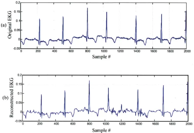
In the previous sections, we examined the performance of CS-based sensor system for a constructed 4-sparse signal. Here, we do the same analysis and evaluations on a real electrocardiogram (ECG) signal obtained from the MIT-BIH Arrhythmia database. Figure 2-9(a) shows a segment of the ECG signal used to evaluate the performance of the systems shown in figure 2-2. Figure 2-9(b) shows the reconstructed signal for the case when

Q

= 12, M = 100 and N = 1000, resulting in a PRD of 0.42%. The minimum required energy versus target PRD curves for the ECG signal

(a) 0 200 400 800 800 1000 1200 1400 1600 1800 2000 Sample # 0. -0.05 0 200 400 600 800 1000 1200 1400 1600 1800 2000 Sample #

Figure 2-9: Original ECG (a) versus CS reconstruction (b) for

Q

12 and M 100.

are plotted for both baseline and CS-based systems. This is a similar result to the case when the input is a constructed 4-sparse signal (see figure 2-5). For target PRD above 1.5% (3.5dB), CS enables about 10X reduction in required energy. It should be noted that in Figure 2-10, PRDg and PRDct are almost identical. This is due to the fact that the used ECG signal is fairly noisy. Hence, both PRDg and PRDact become limited by noise effects and as a result they will be identical.

2.8

Summary

In this chapter, we first looked at the effect of channel noise on the performance of CS-based sensors. We showed how this undesirable effect can be minimized by optimizing the number of measurements and quantization method used in the system.

1000 vuamizarion omy 100 E10 netPRD avgPRD -20 0 20 40 PRD(dB)

Figure 2-10: Minimum energy versus target PRD for an ECG signal from the MIT BIH Arrhythmia database.

In addition to showing robustness to channel noise, we also evaluate the performance of CS-based systems in the presence of input signal noise. We showed that CS-based system is capable of filtering the input noise while the performance of the baseline system (i.e quantization only) will be limited by the input noise. We have also shown that CS can enable on the order of

loX

reduction in transmission energy when compared to the baseline system (i.e. transmitting raw quantized data). Furthermore, we proposed a diversity scheme for CS which requires no additional transmission costs and provides greater than lOX improvement in recovered signal quality. Finally, we showed that the design framework and analysis presented is applicable to real world signals, such as ECGs, with a similar order of magnitude reduction in transmission energy costs.

Chapter 3

Analog to Information Converters

Analog-to-information converters (AICs) have been proposed as a potential so-lution to overcome the resoso-lution and performance limitations of sampling jitter in high-speed analog-to-digital converters (ADC). In this chapter, we compare both en-ergy cost and performance limitations of AIC and high-speed ADC systems, in the context of cognitive radio applications where the input signal is sparse in the fre-quency domain. We explore how jitter and aperture impairments, which commonly limit ADC performance at high sampling frequencies, also impact AIC performance

3.1

Cognitive Radio: An example AIC application

Efficient, high-speed samplers are essential for building modern electronic sys-tems. One such system is cognitive radio, which has been proposed as an intelligent wireless communication protocol for improving the utilization of un-used bandwidth in the radio spectrum [17]. To implement this protocol, the entire radio spectrum has to be simultaneously observed in order to determine the location of used chan-nels. A straightforward approach is to utilize a wideband, Nyquist rate high speed analog-to-digital converter (ADC), however, a severe drawback is that ADCs oper-ating at multi-Giga samples per second (GS/s) require high power and have limited

bit resolution [7, 8]. An alternative approach is to utilize an analog-to-information converter (AIC) based on compressed sensing (CS) techniques [18-26]. Consequently, AICs can relax the frequency requirements of ADCs, potentially enabling higher res-olution and/or lower power receiver front-ends. In general, for applications where signal frequencies are high, but information rates are low, AICs have been proposed as a potential solution to overcome the resolution and performance limitations of traditional, Nyquist-rate high-speed ADCs.

3.1.1

Limitations in High-Speed Sampling

To date, high-speed samplers are used in most of the modern electronic systems [8]. These systems, which work on a variety of signals such as speech, medical imag-ing, radar, and telecommunications, require high-speed samplers, such as high-speed ADCs, to have high bandwidth and significant resolution while working at high fre-quencies (10s of GS/s). Unfortunately, with the current technology, designing high resolution ADCs is highly challenging at such high frequencies. This is mainly due to the fact that these samplers are required to sample at the Nyquist rate (i.e. at least twice the highest frequency component in the signal) to be able to recover the original signal without any loss. Ideally, each sampling event should result in the signal value at the specific sampling instant. However, in practice, there are two main factors that limit the ADC performance: i) uncertainty in the sampling instant, called jitter, and ii) the finite sampling bandwidth, manifested as a weighted integration over a small time interval around the sampling instant, called aperture [27].

As Figure 3-1 shows, the sampling process is really first multiplying with some signal known as sampler signal, and then low pass filtering. The ideal sampler signal would be a delta train with impulses evenly spaced apart at sampling intervals Ts. The non-ideal sampler signal takes into account jitter effects by allowing the interspacing of the impulses to be uneven. The n-th sampling error is given by the difference of

Sampler (A DC)

Sampler Signal Sampler Signal

Ideal Sampler Signal ---

1

(n-1).Ts n.Ts (n+I)Ts

Jittered Sampler Signal

1

(n-1).Ts+En.1 n.Ts+En (n+]).Ts+En.1

Non-ideal Sampler Signal.

(Jitter & Aperture Effect)

Figure 3-1: Ideal and non-ideal sampler, including jitter and aperture effects.

random variable that represents the n-th jitter value. The jitter effect becomes more serious at higher input signal frequencies, as the signal slew-rate (i.e. rate of change of a signal) is proportional to the signal frequency. Thus, a small jitter can cause a significant error in high-speed sampling. We go on to allow the non-ideal sampler signal to further incorporate aperture effects (in addition to the previously described jitter effects). This is also illustrated in Figure 3-1. We model the aperture effect

by replacing the delta impulses in the sampler signal, with triangle pulses, where the

area under the triangle is unity. In reality, the aperture in the sampler is caused by two circuit non-idealities: i) low-pass filtering of the sampler (i.e. limited sampler

A0 Of

A ADIC

01(f)

-- + A -ADC

--A ADC

Figure 3-2: Block diagram of an AIC system.

bandwidth in the signal path), and ii) non-negligible rise/fall time of the clock signal (sampling signal). These non-idealities make the sampler band-limited and cause significant error at high frequencies

[28].

As it was already mentioned, CS has enabled alternative solutions to high-speed ADCs. A well-known example is the AIC. It has been claimed that these AIC ar-chitectures enable high resolution at high frequencies while only using low frequency, sub-Nyquist ADCs [18-26]. In this work, we investigate whether or not AIC sys-tems can indeed resolve both jitter and aperture issues in high-speed samplers, by examining their performance in the presence of these non-idealities.

3.1.2

Analog-to-Information Converter Architecture

While there have been many theoretical discussions on AIC systems in the lit-erature [18-26], to our knowledge, an actual hardware implementation of an AIC system working for wide signal bandwidth (10s of GHz), is yet to be seen. Hence, it is difficult to make a fair hardware-to-hardware comparison with other already implemented high-speed ADCs. In this work, the AIC circuit architecture shown in Figure 3-2 is considered to be compared with a baseline high-speed ADC. In this

ar-chitecture, the input signal f(t) is amplified by using M number of amplifiers. Each signal branch is then individually multiplied with a different pseudorandom number

(PN) waveform <bi(t) to perform CS-type random sampling. The multiplication with

the PN waveform is at Nyquist rate to avoid aliasing in this stage, which we call the mixing stage. At each branch, the mixer output is then integrated over a window of

N sampling periods Ts. Finally, the integrator outputs are sampled and quantized

to form the measurements y, which are then used to reconstruct the original input signal f(t). Note that because we now sample at the rate f/N (see Figure 3-2), this

AIC architecture employs sub-Nyquist rate ADCs, which are less affected by jitter

noise and aperture. The actual advantage over standard ADCs is really unclear until experimentally justified. Also, it is important to point out that the mixing stage still works at the Nyquist frequency, and circuit non-idealities such as jitter and aperture can still be a potential problem in the mixing stage in a manner similar to the sam-pling circuit in high-speed ADCs. In the following section, we present our framework for investigating the impacts of mixer jitter and aperture on AIC performance.

3.2

Evaluation Framework

Figure 3-3(a) shows the block diagram of the AIC system indicating the loca-tion of injected noise due to the jitter and aperture. Figure 3-3(b) shows the same functionality of the AIC system implemented simply using an amplifier and an ADC operating at the Nyquist-rate (N times that of Figure 3-3(a)). This is the system

referred to as the high-speed ADC system, which also suffers from jitter and aperture effects, as illustrated in Figure 3-3(b). The potential advantages of using AICs stem from having a different sensitivity to sources of aperture error and jitter introduced

by different control signals in the AIC system. In the AIC system, the jitter error

from sampling clocks on the slower ADCs, denoted n'(t), is negligible, whereas the main source of error, denoted ni(t), comes from the mixer aperture and the jitter in the PN waveform mixed with the input signal at the Nyquist frequency. On the other

Jitter and Aperture

Effects

(b) fwA> _<D

Figure 3-3: high-speed

Jitter effects in sampling: block diagram of (a) an AIC system, and (b) a

ADC system both with same functionality in the cognitive radio setting.

hand, in the high-speed ADC system, the main source of error is due to the sampling jitter in the high-speed clock. In this section, we provide signal and noise models used to evaluate the performance of these two systems.

3.2.1

Signal Model

The signal model

Nch

f

(t) Z Xj sin(Wj t), (3.1)

j=1

consists of user information coefficients, x, riding on the carriers with frequencies

w (chosen from Nch available channel frequencies in the range of 500 MHz - 20 GHz). This model emulates sparse narrowband or banded orthogonal frequency-division multiplexing communication channels. Our sparsity assumption states that only coefficients xz are non-zero, i.e. only S < Nch users are active at any one time.

(a)

fJl)

3.2.2

Mixer Clocking Jitter

Figure 3-4 shows our jitter noise model where the noise is multiplied by the input signal and filtered in the integrator block. The i-th PN waveform<Di(t) satisfies:

Ts/2 Ideal PN waveform 3 T/2

I

I

-.1 5Ts/2 7Ts/2

il

I

||I

-l | -Jittered PN waveform CD,(t) Jitter-noise Process Ni(t)

II

i

I I

II

II

I

em

mmm

f7L

4

L

m

F

-1

I

I

I

I!

I P

Ii

II

idths

are

||I

||I

ilI

sian distiAbuted 2 ||

Il

||

||

1 1 2 -2

Figure 3-4: Ideal and jittered PN waveforms.

N

<bi(t) = Pijp(t - jTS)

j=1

where

#ij

is the (i,j)-th PN element, and p(t) is a unit height pulse supported on Ts/2 to Ts/2. Denoting the jittered PN waveform as b(t) , then:

Si(t)

= <Di(t) + Ni(t).

Here, Ni(t) is the jitter noise affecting 4(t), described as

N+1

Ni(t) = N-(pi-1 - pi)sgn(E)pj3(t -3 IT, + IE),,

j=-(3.3) (3.2)

I

where the j-th jitter width is ey ~ N(O, -) with o- equal to the jitter root-mean-square (rins), and .j (t, 6)is a unit amplitude pulse supported over the interval [min(0, C), max(0, C)].

To verify 3.3, consider the first transition in the i-th PN waveform <bi(t) in Figure 3-4, where

#io

and

#io

are -1 and 1, respectively. As it is shown, the jitter value Ci at that transition happens to be positive (i.e. PN waveform is shifted to the right due

to jitter). Hence, by using 3.3, the jitter noise Ni(t) at that transition, is a pulse with

a width of c and an amplitude of minus two located at Ts/2.

As a side comment, note that in our model for Ni(t), we assumed that the same phase-locked loop (PLL) is used across all signal paths, resulting in the exact same

jitter sequence c for all jittered PN waveforms J)(t) , 1 <K M i . This model can be extended to include the effect of a longer clock tree distribution, by adding an uncorrelated (or partially correlated) component to each branch, i.e., we would then have a different jitter sequence for each PN waveforms 'bi(t).

3.2.3

Aperture Models

In the AIC system, the aperture is caused by two circuit non-idealities: i) mixers do not operate instantaneously, and ii) the PN waveforms are not ideal. Figure

3-5 illustrates our aperture error model, whereby the aperture effects are captured by the limited rise and fall times in the PN waveform. The aperture error, Di(t),

corresponding to the i-th non-ideal PN waveform

eiJ(t)

, is taken with respect to the i-th jittered PN waveform Si(t), i.e. f(t) = J3(t) + Di(t) . We emphasize that

the reference point for the aperture error is the jittered PN waveform, not the ideal waveform (as was for the jitter noise Ni(t)).

The formula for the i-th aperture error Di(t) is given as:

N+1

Di1(t) ( 2 )q(t - jTs + ++ ), (3.4)

Tr I 1 1 Jittered PN waveform -1 1 -1 CD,(t)I 11 Non-ideal PN I waveform -1 I-1 -1

<(t)

Aperture Error D,(t) -1| -1 -1

Figure 3-5: Aperture error caused by non-ideal PN waveform.

where

#hj

is the (i,j)-th PN element, and q(t) can be described as:

2+ 1) -9_ < t < 0

q(t) - L - 1 <t< (3.5)

0 otherwise

where T, is the parameter that dictates the rise/fall time of the PN waveform. Similar to the jitter noise, the aperture error Di(t) is also multiplied by the input signal and filtered in the integrator block.

3.2.4

Reconstruction of Frequency Sparse Signal

Using the described CS framework in chapter 2 , we now frame the reconstruction problem for the AIC. As Figure 3-3(a) shows, each measurement y, is computed by

integrating the noise,ni(t) = f(t) -(Ni(t) + Di(t)), and the product of the signal f(t)

and the PN waveform 4Gi(t), as follow:

N.Ts+T,|2 yi = _J Ts 2

f

(t) - 4Ji (t)dt + N-Ts+T ,|2

J

n (t) dt. T/2

Substituting the signal model from 3.1, the measurements can be shown to satisfy y = JNJx + no, where PN matrix D has entries

#ij

and

N-T,+T,|2 n= T/2 i.Ts+T,|2 IFij = I si (i-1).Ts+T,|2 N-Ts+Ts|2 ni (t)dt= Ts/2

where no = (n , n", ..., nM)". Here, the noise no is merely the projection of

f(t)

by the i-th jitter noise pulse process Ni(t) and i-th aperture error pulse Di(t) (see Figure 3-4 and Figure 3-5).

In the next section, we use our noise model and reconstruction framework to compare the performance of AIC versus high-speed ADC systems.

3.3

Evaluation Results

For our signal f(t), refer to model 3.1, we assume 1000 possible subcarriers (i.e.

Nch = 1000). We test our system using a randomly generated signal f(t), where S non-zero values are drawn from a uniform random distribution over [0, 1] to assign the information coefficients xi, and S integer values are drawn from a uniform random distribution over [1, Nch] to assign subcarrier (channel location) of S active users.

To compare the performance of the high-speed ADC and the AIC systems, we

(3.6)

n(wj t) dt

f

(t) -(Ni (t) +Di (t)) dt

(3.7)

adopt the same ENOB metric from ADC literature, which is defined as:

ENOB = log2

(

*w*n , (3.9)

(f - f

-2

)

where Ving is the full-scale input voltage range of the ADCs and

f

-

f

is the rms signal distortion (use fq in place of f for the high-speed ADC system in Figure 3-3(b)). In order to illustrate the relative impact of jitter and aperture, we first ignore aperture effects, and limit our evaluation results to only jitter limited systems. We later add aperture effects to the jitter noise, and observe the differences.

3.3.1

Jitter-limited ENOB

The jitter-limited ENOB for both systems is plotted in Figure 3-6. As the number of non-zero components of x, S, increases, we see that the AIC performance worsens while the high-speed ADC performance improves. The reasons for this are as follows. In the receiver, the input signal f(t) peaks are always normalized to Vsminq, the full-scale voltage range of the ADC. When S increases, this normalization causes the coefficient values xjI| to get smaller with respect to Vswing. In the high-speed ADC system, the jitter-error is dominated by the coefficient

Ixzl

corresponding to the highest input frequency and the error drops if the coefficient value drops. Hence, ENOB increases since increases with S, see 3.9. On the other hand, the AIC system has a different behavior. As S increases, the reconstruction performs worse and as a result AIC distortion gets worse, resulting in poorer ENOB performance. As shown in Figure 3-6, when we consider only the impact of jitter, the AIC system can improve the ENOB by 1 and 0.25 bits for S of 1 and 2, respectively. For signals with higher S, the high-speed ADC performs better than the AIC system. As a point of reference, the standard Walden curve [7] is also plotted in Figure 3-6, which depicts the ADC performance with input signal at Nyquist frequency. We see that compared to the Walden curve, the high-speed ADC can actually achieve a better resolution

(a) 16 14 14 ADC, 12 -AIC, S=2 10-0 AIC, S=1 8 A 6-4 Nyquist ADC (b) 10 1 Jitter (rms) 16 14 12 10- ADC, 3 105

z AIC, S=5 ADC, S=10&12

AIC, S=10 Nyquist ADC-6 AIC, S=12 2-5-14 _{-13 1} 10~ 10 Jitter (rms) 101

Figure 3-6: Jitter (rms) versus ENOB for (a) S = _{1, 2, and (b) S = 5, 10, 12, (N=1000,}

M = 100 for all S).

(i.e. the Walden curve is a pessimistic estimate). This is due to the fact that the input signal, f(t), does not always have all its spectra concentrated at the Nyquist