HAL Id: hal-00124582
https://hal.archives-ouvertes.fr/hal-00124582
Submitted on 15 Jan 2007
HAL is a multi-disciplinary open access
archive for the deposit and dissemination of
sci-entific research documents, whether they are
pub-lished or not. The documents may come from
teaching and research institutions in France or
abroad, or from public or private research centers.
L’archive ouverte pluridisciplinaire HAL, est
destinée au dépôt et à la diffusion de documents
scientifiques de niveau recherche, publiés ou non,
émanant des établissements d’enseignement et de
recherche français ou étrangers, des laboratoires
publics ou privés.
Probing the structure of protoplanetary disks: a
comparative study of DM Tau, LkCa 15 and MWC 480
Vincent Piétu, Anne Dutrey, S. Guilloteau
To cite this version:
Vincent Piétu, Anne Dutrey, S. Guilloteau. Probing the structure of protoplanetary disks: a
compar-ative study of DM Tau, LkCa 15 and MWC 480. Astronomy and Astrophysics - A&A, EDP Sciences,
2007, 467 (1), pp.163-178. �hal-00124582�
hal-00124582, version 1 - 15 Jan 2007
January 15, 2007
Probing the structure of protoplanetary disks: a comparative
study of DM Tau, LkCa 15 and MWC 480
Vincent Pi´etu
1,2, Anne Dutrey
1and St´ephane Guilloteau
11 Universit Bordeaux 1 ; CNRS ; OASU ; UMR 5804, BP 89, 2 rue de l’Observatoire, F-33270 Floirac, France
2 Institut de Radio-Astronomie Millim´etrique, 300 rue de la Piscine, Domaine Universitaire F-38406 Saint Martin d’H`eres, France
Received 11-Oct-2006, Accepted 08-Jan-2007
ABSTRACT
Context.The physical structure of proto-planetary disks is not yet well constrained by current observations. Millimeter interferometry is an essential tool to investigate young disks.
Aims.We study from an observational perspective the vertical and radial temperature distribution in a few well-known disks. The surface density distribution of CO and HCO+and the scale-height are also investigated.
Methods.We report CO observations at sub-arcsecond resolution with the IRAM array of the disks surrounding MWC 480, LkCa 15 and DM Tau, and simultaneous measurements of HCO+
J=1→0. To derive the disk properties, we fit to the data a standard disk model in which all parameters are power laws of the distance to the star. Possible biases associated to the method are detailed and explained. We compare the properties of the observed disks with similar objects.
Results.We find evidence for vertical temperature gradient in the disks of MWC 480 and DM Tau, as in AB Aur, but not in LkCa 15. The disks temperature increase with stellar effective temperature. Except for AB Aur, the bulk of the CO gas is at temperatures smaller than 17 K, below the condensation temperature on grains. We find the scale height of the CO distribution to be larger (by 50%) than the expected hydrostatic scale height. The total amount of CO and the isotopologue ratio depends globally on the star. The more UV luminous objects appears to have more CO, but there is no simple dependency. The [13CO]/[HCO+
] ratio is ∼ 600, with substantial variations between sources, and with radius. The temperature behaviour is consistent with expectations, but published chemical models have difficulty reproducing the observed CO quantities. Changes in the slope of the surface density distribution of CO, compared to the continuum emission, suggest of a more complex surface density distribution than usually assumed in models. Vertical mixing seems an important chemical agent, as well as photo-dissociation by the ambient UV radiation at the disk outer edge.
Key words.Stars: circumstellar matter – planetary systems: protoplanetary disks – individual: LkCa 15, MWC 480, DM Tau – Radio-lines: stars
1. Introduction
CO rotation line observations of low-mass and intermediate-mass Pre-Main-Sequence (PMS) stars in Taurus-Auriga (∼ 140 pc, Kenyon et al., 1994) provide strong evidences that both TTauri and Herbig Ae stars are surrounded by large (Rout ∼ 200 − 800 AU) Keplerian disks (GM Aur: Koerner et al.
(1993), GG Tau: Dutrey et al. (1994), MWC 480: Mannings et al. (1997)). Differences between TTauri and Herbig Ae disks are observed in the very inner disk, very close to the star (Dullemond et al. 2001; Monnier & Millan-Gabet 2002). However, detailed comparisons, namely based on resolved ob-servations instead of SED analysis, between Herbig Ae disks
Send offprint requests to: V.Pi´etu, e-mail: [email protected]
1 Based on observations carried out with the IRAM Plateau de Bure Interferometer. IRAM is supported by INSU/CNRS (France), MPG (Germany) and IGN (Spain).
and TTauri disks are too few to allow conclusions about the whole disk. In particular, there is no specific study on the in-fluence of the spectral type on the disk properties. This can be achieved by comparing the properties of outer disks imaged by millimeter arrays.
The first rotational lines of CO (J=1-0 and J=2-1) mostly trace the cold gas located in the outer disk (R > 30 AU) since current millimeter arrays are sensitivity limited and do not al-low the detection of the warmer gas in the inner disk. In the last years, several detailed studies of CO interferometric maps have provided the first quantitative constrains on the physical prop-erties of the outer disks. Among them, the method developed by Dartois et al. (2003) is so far the only way to estimate the overall gas disk structure. Dartois et al. (2003) deduced the ver-tical temperature gradient of the outer gas disk of DM Tau from a multi-transition, multi-isotope analysis of CO J=1-0 and J=2-1 maps. The dust distribution and its temperature can be traced
by IR and optical observations and SED modelling (D’Alessio et al. 1999; Dullemond & Dominik 2004). However Pi´etu et al. (2006) recently demonstrated that SED analysis are limited by the dust opacity. Due to the high dust opacity in the optical and in the IR, only the disk surface is properly characterized. Images in the mm domain, where the dust is essentially opti-cally thin, revealed in the case of MWC 480 a dust temperature which is significantly lower than those inferred from SED anal-ysis and from CO images. With ALMA, the method described in this paper, which is today only relevant to the outer disk, will become applicable to the inner disk of young stars.
In this paper, we focus on the gas properties deduced from CO data. The analysis of the millimeter continuum data, ob-served in the meantime, is presented separately (Pi´etu et al. 2006)). Here, we generalize the method developed by Dartois et al. (2003) and we apply it to two Keplerian disks surround-ing the TTauri star LkCa 15 (spec.type K5, Duvert et al. 2000) and the Herbig Ae star MWC 480 (A4 spectral type, Simon et al. 2000). By improving the method, we also discuss the es-timate of disk scale heights. Then, we compare their proper-ties with those surrounding Herbig Ae and TTauri disks such as AB Aur (Pi´etu et al. 2005), HD 34282 (Pi´etu et al. 2003), DM Tau (Dartois et al. 2003).
After presenting the sample of stars and the observations in Sect. 2, we describe the improved analysis method in Sect. 3. Results are presented in Sect. 4 and their implications discussed in Sect. 5.
2. Sample of Stars and Observations
2.1. Sample of Stars
The stars were selected to sample the wider spectral type range with only a few objects. Table 1 gives the coordinates and spec-tral type of the observed stars, as well as of HD 34282 and GM Aur which were observed in12CO by Pi´etu et al. (2003)
and Dutrey et al. (1998) respectively. Our stars have spectral type ranging from M1 to A0. All of them have disks observed at several wavelengths and are located in a hole or at the edge of their parent CO cloud.
DM Tau: DM Tau is a bona fide T Tauri star. Guilloteau & Dutrey (1994) first detected CO lines indicating Keplerian rotation using the IRAM 30 meter telescope. Guilloteau & Dutrey (1998) have confirmed those findings by resolving the emission of the 12CO J=1→0 emission using IRAM Plateau de Bure interferometer (PdBI) and derived physical parame-ters of its protoplanetary disk and mass for the central star. Dartois et al. (2003) performed the first high resolution multi-transition, multi-isotope study of CO, and demonstrated the ex-istence of a vertical temperature gradient in the disk.
LkCa 15: This is a CTT isolated from its parent cloud. Duvert et al. (2000) and Qi et al. (2003) observed the disk in12CO and
in HCO+. High resolution12CO data was obtained by Simon
et al. (2000) who used it to derive the stellar mass.
MWC 480: The existence of a disk around this A4 Herbig Ae star was first reported by Mannings et al. (1997). Using data from OVRO, they perform a modelling of the gas disk consis-tent with Keplerian rotation. More recently, Simon et al. (2000) confirmed that the rotation was Keplerian and measured the stellar mass from the CO pattern.
AB Aurigae: AB Aur is considered as the proto-type of the Herbig Ae star (of spectral type A0) which is surrounded by a large CO and dust disk. The reflection nebula, observed in the optical, extends far away from the star (Grady et al. 1999). Semenov et al. (2005) used the 30-m to observe the chemistry of the envelope. Pi´etu et al. (2005) has analyzed the disk us-ing high angular resolution images of CO and isotopologues from the IRAM array and found that, surprisingly, the rotation is not Keplerian. A central hole was detected in the continuum images and in the more optically thin13CO and C18O lines.
2.2. PdBI data
For DM Tau, LkCa 15, and MWC 480, the 12CO J=2-1 data
were observed in snapshot mode during winter 1997/1998 in D, C2 and B1 configurations. Details about the data quality and reduction are given in Simon et al. (2000) and in Dutrey et al. (1998). The 12CO J=2-1 data were smoothed to 0.2 km.s−1
spectral resolution. The HCO+
J=1→0 data were obtained si-multaneously: a 20 MHz/512 channels correlator unit provided a spectral resolution of 0.13 km.s−1. The13CO J=1-0 and
J=2-1 observations of DM Tau are described in Dartois et al. (2003). We obtained complementary 13CO J=2-1 and J=1-0 (to-gether with C18O J=1-0 observations) of MWC 480 and LkCa 15. These observations were carried out in snapshot mode (partly sharing time with AB Aur) in winter periods be-tween 2002 and 2004. Configurations D, C2 and B1 were used at 5 antennas. MWC 480 has also shortly been observed in A configuration simultaneously with AB Aur. Finally, data was obtained in the largest A+configuration for LkCa 15 and
MWC 480 in January 2006 (for a description of these observa-tions, see Pi´etu et al. 2006). Both at 1.3 mm and 2.7 mm, the tuning was double-side-band (DSB). The backend was a cor-relator with one band of 20 MHz, 512 channels (spectral res-olution 0.11 km.s−1) centered on the13CO J=1-0, one on the
C18O J=1-0 line, and a third one centered on the13
CO J=2→1 line (spectral resolution 0.05 km.s−1), and 2 bands of 160 MHz for each of the 1.3 mm and 2.7 mm continuum. The phase and secondary flux calibrators were 0415+379 and 0528+134. The rms phase noise was 8◦ to 25◦and 15◦ to 50◦ at 3.4 mm and 1.3 mm, respectively (up to 70◦on the 700 m baselines), which introduced position errors of ≤ 0.05′′. The estimated seeing is
about 0.2′′.
Flux density calibration is a critical step in such projects. The kinetic temperature which is deduced from the modelling is directly proportional to the measured flux density. This is even more problematic since we compare data obtained on sev-eral years. Hence, we took great care of the relative flux cali-bration by using not only MWC 349 as a primary flux refer-ence, assuming a flux S(ν) = 0.95(ν/87GHz)0.60(see the IRAM
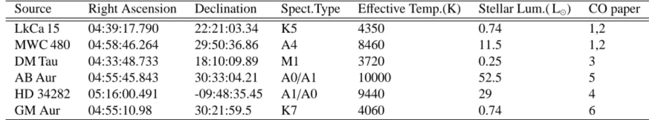
Table 1. Star properties
Source Right Ascension Declination Spect.Type Effective Temp.(K) Stellar Lum.( L⊙) CO paper
LkCa 15 04:39:17.790 22:21:03.34 K5 4350 0.74 1,2 MWC 480 04:58:46.264 29:50:36.86 A4 8460 11.5 1,2 DM Tau 04:33:48.733 18:10:09.89 M1 3720 0.25 3 AB Aur 04:55:45.843 30:33:04.21 A0/A1 10000 52.5 5 HD 34282 05:16:00.491 -09:48:35.45 A1/A0 9440 29 4 GM Aur 04:55:10.98 30:21:59.5 K7 4060 0.74 6
Col. 2,3: J2000 coordinates deduced from the fit of the 1.3 mm continuum map of the PdBI. Errors bars on the astrometry are of order ≤ 0.05′′.
Col. 4,5, and 6, the spectral type, effective temperature and the stellar luminosity are those given in Simon et al. (2000) and Pi´etu et al. (2003) for HD 34282 and van den Ancker et al. (1998) for AB Aur. Col.6, list of CO interferometric papers are: 1 = this paper, 2 = Simon et al. (2000), 3 = Dartois et al. (2003), 4 = Pi´etu et al. (2003), 5 = Pi´etu et al. (2005), 6 = Dutrey et al. (1998).
flux report 14) but also by having always our own internal ref-erence in the observations. For this purpose we applied two methods: i) we used MWC 480 as a reference because its con-tinuum emission is reasonably compact and bright, ii) we also checked the coherency of the flux calibration on the spectral in-dex of DM Tau, as described in Dartois et al. (2003). We cross-checked all methods and obtained by these ways a reliable rel-ative flux calibration from one frequency to another.
2.3. Data Reduction and Results
We used the GILDAS1 software package (Pety 2005) to re-duce the data and as a framework to implement our min-imization technique. Figure 1 presents some channel maps of 12CO, 13
CO J=2→1 and 13
CO J=1→0 for LkCa 15 and MWC 480. Similar figures for DM Tau can be found in Dartois et al. (2003), and for AB Aur in Pi´etu et al. (2005). A veloc-ity smoothing to 0.6 km.s−1(for MWC 480) and 0.4 km.s−1 (for LkCa 15) was applied to produce the images displayed in Fig.1. However, in the analysis done by minimization, we used spectral resolutions of 0.20 km.s−1(12CO and HCO+) and 0.21
km.s−1(13CO), and natural weighting was retained.
The HCO+images are presented in Fig.2. The typical
an-gular resolution of these images is 3 − 4′′. For LkCa 15, the line
flux is compatible with the result quoted by Duvert et al. (2000) and Qi et al. (2003), and for DM Tau with the single-dish mea-surement of Dutrey et al. (1997).
3. Model description and Method of Analysis
In this section, we summarize the model properties and de-scribe the improvements since the first version (Dutrey et al. 1994).
3.1. Solving the Radiative Transfer Equation
To solve the radiative transfer equation coupled to the statis-tical equilibrium, we have written a new code, offering non LTE capabilities. More details are given in Pavlyuchenkov et al. (2007). The LTE part, which is sufficient for low energy level
1 See http://www.iram.fr/IRAMFR/GILDAS for more informa-tion about the GILDAS softwares.
of rotational CO lines (J=1-0 and J=2-1), is strictly similar to that of Dutrey et al. (1994), and uses ray-tracing to compute the images. The HCO+data was also analyzed in LTE mode (see
Sect.3.2.3 for the interpretation of this assumption). We use a scheme of nested grids with regular sampling to provide suf-ficient resolution in the inner parts of the disk while avoiding excessive computing time.
3.2. Description of the physical parameters
For each spectral line, the relevant physical quantities which control the line emission are assumed to vary as power law as function of radius (see Sect.3.2.1 for the interpretation of this term) and, except for the density, do not depend on height above the disk plane. The exponent is taken as positive if the quantity decreases with radius:
a(r) = a0(r/Ra)−ea
For each molecular line, the disk is thus described by the fol-lowing parameters :
– X0,Y0, the star position, and Vdisk, the systemic velocity.
– PA, the position angle of the disk axis, and i the inclination. – V0, the rotation velocity at a reference radius Rv, and v the
exponent of the velocity law. With our convention, v = 0.5 corresponds to Keplerian rotation. Furthermore, the disk is oriented so that the V0is always positive. Accordingly, PA
varies between 0 and 360◦, while i is constrained between
−90◦and 90◦(see fig. 3).
– Tmand qm, the temperature value at a reference radius RT
and its exponent (see Sect.3.2.3).
– dV, the local line width, and its exponent ev. The
interpre-tation of dV is discussed in Sect.3.2.6
– Σm, the molecular surface density at a radius RΣand its
ex-ponent pm
– Rout, the outer radius of the emission, and Rin, the inner
radius.
– hm, the scale height of the molecular distribution at a
ra-dius Rh, and its exponent eh: it is assumed that the density
distribution is Gaussian, with
n(r, z) = Σ(r) h(r)√πexp
h
Fig. 1. Channel maps of the12CO and13CO line emission towards MWC 480 and LkCa 15. The synthesized beam is indicated in
each panel. The cross indicates the direction of the major and minor axis of each disk, as respectively derived from the analysis of the line data. The velocity of the channel is indicated in the upper left corner of each panel (LSR velocity in km.s−1). A
200 m taper has been applied on the13
CO J=2→1 data of LkCa 15 which where obtained at higher angular resolution. Left: MWC 480 Left:12
CO J=2→1 line, spatial resolution 1.38 × 0.99′′at PA 16◦, contour spacing 200 mJy/beam, or 3.4 K, or 3.6
σ. Middle:13CO J=2→1 line, spatial resolution 0.77 × 0.57 at PA 26◦, contour spacing 50 mJy/beam, or 2.9 K, or 1.9 σ. Right:
13
CO J=1→0 line, spatial resolution 1.72 × 1.24′′at PA 37◦, contour spacing 20 mJy/beam, or 0.9 K, or 1.8 σ. Negative contours are dashed, and the zero contour is omitted. Right: LkCa 15 Left:12CO J=2→1 line, spatial resolution 2.01 × 1.20′′at PA 12◦, contour spacing 150 mJy/beam, or 1.4 K, or 2.5 σ. Middle:13
CO J=2→1 line, spatial resolution 1.46 × 1.24 at PA 52◦, contour
spacing 100 mJy/beam, or 1.4 K, or 1.6 σ. Right:13
CO J=1→0 line, spatial resolution 2.55 × 1.51′′at PA 47◦, contour spacing
30 mJy/beam, or 0.8 K, or 1.8 σ. Negative contours are dashed, and the zero contour is omitted.
(note that with this definition, eh<0 in realistic disks)
thus giving a grand total of 17 parameters to describe the emis-sion.
It is important to realize that all these parameters can ac-tually be constrained for the lines we have observed, under the above assumption of power laws. This comes from two specific properties of proto-planetary disks: i) the rapid decrease of the surface density with radius, and ii) the known kinematic
pat-tern. The only exception is the inner radius, Rin, for which an
upper limit of typically 20 – 30 AU can only be obtained. The use of power laws is appropriate for the velocity, pro-vided the disk self-gravity remains small. Power laws have been shown to be a good approximation for the kinetic temper-ature distribution (see, e.g. Chiang & Goldreich 1997), and thus to the scale height prescription. For the surface density, power laws are often justified for the mass distribution based on the α prescription of the viscosity with a constant accretion rate:
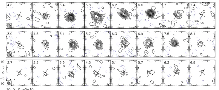
self-Fig. 2. Channel maps of the HCO+
J=1→0 line emission towards DM Tau, LkCa 15 and MWC 480. The cross indicates the direction of the major and minor axis of each disk. The velocity of the channel is indicated in the upper left corner of each panel (LSR velocity in km.s−1). For displaying purpose, the spectral resolution is 0.6 km.s−1for MWC 480 and LkCa 15, and 0.4
km.s−1for DM Tau. All contour steps are 20 mJy/beam (∼ 2σ), negative contours are dashed and the zero contour is omitted. Top: DM Tau, spatial resolution is 4.3 × 3.3′′at PA 47◦, contour step 0.22 K. Middle: LkCa 15, spatial resolution is 4.6 × 3.4′′at
PA 19◦, contour step 0.25 K. Bottom: MWC 480, spatial resolution is 3.5 × 2.5′′at PA 42◦, contour step 0.36 K.
similar solutions to the disk evolution imply power laws with an exponential edge (Hartmann et al. 1998). Although Malbet et al. (2001) pointed out some limitations of this assumption for the inner parts (r < 30 AU) of the disk, the approximation re-mains reasonable beyond 50 AU. However, although this may be valid for H2, chemical effects may lead to significant
dif-ferences for any molecule. Given the limited spatial dynamic range and signal to noise provided by current (sub-)millimeter arrays, using more sophisticated prescriptions is not yet justi-fied, and power laws offer a first order approximation of the overall molecular distribution.
3.2.1. Spherical vs Cylindrical representation
To describe the disk and its parameters, we can use either cylin-drical or spherical coordinates.
The description given in the previous sub-section is unam-biguous for thin disks (where h(r) ≪ r), However, for molec-ular disks with outer radius as large as 800 AU, the disk thick-ness is no longer small, and the classical theory of hydrostatic scale height, which uses cylindrical coordinates, is only valid in the small h/r limit. It may then become significant to distin-guish between a spherical representation, where the functions depends on the distance to the star (r = d) and height above disk plane, z
F = f (d, z) (2) and a cylindrical representation, where the functions depends on the projected distance on the disk (r = ρ) and height z
F = f (ρ, z) (3) with d2= ρ2+ z2. It is obvious that the exponent of the power
laws will depend slightly on which description is selected. We
have evaluated the differences between the two different repre-sentations (see Tab.2): as expected, the results are very similar for 13
CO, but the cylindrical representation is a ∼ 8 sigma bet-ter representation for 12
CO J=2→1 (the most affected transi-tion because of its higher opacity). The most affected param-eters are Σ and h. However, with the exception of the scale height, the effects remain small compared to the uncertainties. Accordingly, we have arbitrarily decided to represent all pa-rameters in terms of cylindrical laws, i.e. the radius is r = ρ in the model description.
3.2.2. Reference Radius
Unless pm≃ 0, the choice of the reference radius RΣwill affect
the relative error bar on Σm, δΣm/Σm. Depending on the
an-gular resolution and on the overall extent of the emission, for each molecular line, there is a different optimal radius RΣwhich
minimizes this relative error. The same is true for all other ref-erence radii for the power laws. This makes direct comparison at an arbitrary radius not straightforward. To circumvent this problem, we have determined Σm, δΣmas a function of the
ref-erence radius for each transition, and selected the RΣgiving the
best S/N ratio. Results are given Fig.4-6: note that the curves
Σm(RΣ) should not be interpreted as independent estimates of
the local surface density at different radii: they explicitly rely on the assumption of a single power law throughout the whole disk.
The same arguments can be applied to all other power laws, in particular to the scale height and the temperature. However, for the latter, the exponent is usually small (q = −0.2 − 0.5), so the choice of the reference radius is less critical. Figure 4 shows the variation of the parameters (here Σm, Tmand h) and
ra-00000000000 00000000000 00000000000 00000000000 00000000000 00000000000 00000000000 00000000000 00000000000 00000000000 00000000000 00000000000 00000000000 00000000000 00000000000 11111111111 11111111111 11111111111 11111111111 11111111111 11111111111 11111111111 11111111111 11111111111 11111111111 11111111111 11111111111 11111111111 11111111111 11111111111 00000000000 00000000000 00000000000 00000000000 00000000000 00000000000 00000000000 00000000000 00000000000 00000000000 00000000000 00000000000 00000000000 00000000000 00000000000 11111111111 11111111111 11111111111 11111111111 11111111111 11111111111 11111111111 11111111111 11111111111 11111111111 11111111111 11111111111 11111111111 11111111111 11111111111 axis Disc axis Disc axis Disc axis Disc 00000000000 00000000000 00000000000 00000000000 00000000000 00000000000 00000000000 00000000000 00000000000 00000000000 00000000000 00000000000 00000000000 00000000000 00000000000 11111111111 11111111111 11111111111 11111111111 11111111111 11111111111 11111111111 11111111111 11111111111 11111111111 11111111111 11111111111 11111111111 11111111111 11111111111 00000000000 00000000000 00000000000 00000000000 00000000000 00000000000 00000000000 00000000000 00000000000 00000000000 00000000000 00000000000 00000000000 00000000000 00000000000 11111111111 11111111111 11111111111 11111111111 11111111111 11111111111 11111111111 11111111111 11111111111 11111111111 11111111111 11111111111 11111111111 11111111111 11111111111 PA PA North North i > 0 i > 0 i < 0 i < 0 North PA North PA 00000000 00000000 00000000 00000000 00000000 00000000 00000000 00000000 00000000 00000000 00000000 00000000 00000000 00000000 00000000 00000000 00000000 00000000 00000000 00000000 00000000 00000000 00000000 00000000 00000000 11111111 11111111 11111111 11111111 11111111 11111111 11111111 11111111 11111111 11111111 11111111 11111111 11111111 11111111 11111111 11111111 11111111 11111111 11111111 11111111 11111111 11111111 11111111 11111111 11111111 00000000 00000000 00000000 00000000 00000000 00000000 00000000 00000000 00000000 00000000 00000000 00000000 00000000 00000000 00000000 00000000 00000000 00000000 00000000 00000000 00000000 00000000 00000000 00000000 00000000 11111111 11111111 11111111 11111111 11111111 11111111 11111111 11111111 11111111 11111111 11111111 11111111 11111111 11111111 11111111 11111111 11111111 11111111 11111111 11111111 11111111 11111111 11111111 11111111 11111111 0000000 0000000 0000000 0000000 0000000 0000000 0000000 0000000 0000000 0000000 0000000 0000000 0000000 0000000 0000000 0000000 0000000 0000000 0000000 0000000 0000000 0000000 0000000 0000000 0000000 0000000 1111111 1111111 1111111 1111111 1111111 1111111 1111111 1111111 1111111 1111111 1111111 1111111 1111111 1111111 1111111 1111111 1111111 1111111 1111111 1111111 1111111 1111111 1111111 1111111 1111111 1111111 00000000 00000000 00000000 00000000 00000000 00000000 00000000 00000000 00000000 00000000 00000000 00000000 00000000 00000000 00000000 00000000 00000000 00000000 00000000 00000000 00000000 00000000 00000000 00000000 00000000 00000000 11111111 11111111 11111111 11111111 11111111 11111111 11111111 11111111 11111111 11111111 11111111 11111111 11111111 11111111 11111111 11111111 11111111 11111111 11111111 11111111 11111111 11111111 11111111 11111111 11111111 11111111
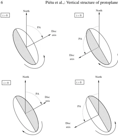
Fig. 3. Geometrical convention: four disk configurations yield-ing the same aspect ratio when projected are presented. The shaded area correspond to the part of the disk that is closer to us than the plane of the sky containing the disk axis. The curved arrow represents the sense of rotation (this defines the disk axis). The projected velocities allow to disentangle be-tween one of the two columns (for the two cases presented on the left, the red-shifted part would be the lower part, and the contrary for the two cases on the right). It is possible to deter-mine the sign of the inclination either with the asymmetry at the systemic velocity if sufficient signal to noise is available, or by other means, e.g. scattered images in the optical and near-IR. PA is classically designed to be positive East from North.
dius for DM Tau. This is a reanalysis of the data published by Dartois et al. (2003). This method gives consistent results with previous work, but allows a more precise determination of the parameters (especially the surface density as stated above), by determining in which region they are constrained. Fig.4 indi-cates that the temperature is determined around 100 – 200 AU, while the surface densities are constrained in the 300 – 500 AU region. Somewhat smaller values apply to the other sources, LkCa 15 and MWC 480 (see Fig.5-6).
3.2.3. Temperature law
The interpretation of Tm(and as a consequence of Σm) depends
on the specific model of radiative transfer being used. In this paper, we are dealing with CO isotopologues, for which LTE is good approximation: Tmis then the kinetic temperature. For
transitions which may not be thermalized, two different radia-tive transfer models may be used. We can apply an LTE ap-proximation: since we are fitting brightness distributions, Tmis
Table 2. Cylindrical vs Spherical description
Line 13CO(1-0) 13CO(2-1) 12CO(2-1)
Cylindrical Rout(AU) 791 ± 33 725 ± 24 868 ± 15 T0(K) 9.1 ± 0.3 14.7 ± 0.3 24.2 ± 0.2 q −0.17 ± 0.09 0.18 ± 0.05 0.46 ± 0.01 V0(km.s−1) 2.12 ± 0.07 2.02 ± 0.06 2.09 ± 0.06 v 0.5 0.5 0.5 dV (km.s−1) 0.133 ± 0.015 0.136 ± 0.015 0.147 ± 0.010 ev −0.28 ± 0.08 −0.04 ± 0.07 0.08 ± 0.04 Σm(cm−2) 26.9 ± 1.7 1016 41.4 ± 6.1 1016 37.4 ± 9.1 1018 pm 3.3 ± 0.3 3.7 ± 0.4 4.5 ± 0.5 hm(AU) 27.1 ± 4.4 27.8 ± 2.9 33.4 ± 2.3 eh −1.07 ± 0.20 −1.09 ± 0.10 −0.99 ± 0.04 χ2 513329.3 514557.2 136376.5 Spherical Rout 804 ± 34 737 ± 20 898 ± 12 T0 9.3 ± 0.3 15.2 ± 0.4 26.7 ± 0.2 q −0.14 ± 0.09 0.20 ± 0.05 0.50 ± 0.01 V0(km.s−1) 2.16 ± 0.07 2.07 ± 0.06 2.08 ± 0.05 v 0.5 0.5 0.5 dV (km.s−1) 0.135 ± 0.016 0.137 ± 0.015 0.183 ± 0.012 ev −0.26 ± 0.08 −0.05 ± 0.06 0.17 ± 0.05 Σm(cm−2) 25.7 ± 1.8 1016 35.1 ± 5.3 1016 41.1 ± 7.4 1017 pm 3.2 ± 0.3 3.6 ± 0.4 3.4 ± 0.4 hm(AU) 20.7 ± 2.2 23.4 ± 2.4 19.7 ± 1.4 eh −1.32 ± 0.18 −1.13 ± 0.12 −1.25 ± 0.06 χ2 513329.5 514558.9 136451.5
Results for DM Tau with “free” scale-height and “free” line-width (see Sect. 3.2.5 and 3.2.6 for more details) in the cylindrical and spherical representations. Caution: this table is here to illustrate the dependence on the geometry of as many parameters as possible. The best parame-ters to be applied to DM Tau should be taken from Table 3.
in this case the excitation temperature Tex, and the surface
den-sity Σmis computed assuming the same temperature controls all
level population, i.e. the partition function. We can also solve for molecular line excitation using a non-LTE statistical equi-librium code: Tm is then the kinetic temperature, and Σm the
total molecule surface density, within the limitations of the ra-diative transfer code accuracy. In this paper, only the LTE mode was used.
3.2.4. Surface Density
The surface density is expected to fall off rapidly with distance from the star (p(H2) ≃ 1 − 2), and in particular much more
rapidly than the temperature (q ≃ 0.5). Remembering that, be-cause of the partition function, the line opacity of a J = 1 − 0 transition scales as Σm/T2 at high enough temperatures (for
constant line width), this indicates that, in general, the central part of the disk is much more optically thick than the outer regions. For the detectable lines, the temperature can be de-rived from the emission from this optically thick core, while the surface density Σmis derived from the optically thin region.
This remains valid provided the same temperature law applies to the two regions. For the weakest lines, the optically thick
core may be too small, and the temperature exponent remains essentially unconstrained: this should be reflected to by the er-ror bars on the temperature. In such cases, however, the line emission scales as Σm/T (for J=1-0 line).
If the molecule is very abundant, such as CO, the local line core may be optically thick almost throughout the disk. However, the local line wings remain optically thin: if the ve-locity resolution is high enough, this information can be used to constrain the opacity, and hence the surface density, although less accurately. To illustrate this point, let us consider the case of a face on disk. The apparent width of the line profile is then controlled only by the internal velocity dispersion (turbulent + thermal) and by the line opacity. In the outer parts, the line is optically thin and of Gaussian shape, while in the inner parts, the line is broadened by the large opacity, and the profile tends towards a square shape, with width proportional to √ln(τ). The evolution of the line profiles as function of radius indicates at which radius τ = 1, and thus constrains the molecular sur-face density. Note that if the spectral resolution is insufficient to properly sample the line width, this is no longer possible. Current correlators are not instrumentally limited but smooth-ing can be necessary when the sensitivity is the limitsmooth-ing factor. If the disk is not seen face on, the systematic velocity gradi-ent get superimposed to this local line broadening, but does not change the fundamental relationship between the apparent (lo-cal) line width and the opacity. In any case, since the effect goes as √ln(τ), measuring the surface density by such a method is expected to be rather unprecise, and will result in larger errors. Furthermore, it should be noted that this opacity broadening effect results in a slight coupling of the line width parameters,
dV and ev, to the surface density.
3.2.5. Scale Height
The existence of a known kinematic pattern also allows to con-strain the scale height parameters h0and eh. Unless the disk is
seen face on, for an optically thin line, the velocity range inter-sected along a line of sight will depend on the disk inclination and flaring, resulting in a coupling between scale height and line width. For an optically thick line, the difference in inclina-tions between the front and back regions of the disk can also be measured. The spatial distribution of the emission as a func-tion of projected velocity (or funcfunc-tion of the velocity channels) along the line of sight will depend on the scale height of the disk (this is illustrated for the opacity by Fig.3 from Dartois et al. (2003)). At first glance, the expected scale heights, of or-der 50 AU at 300 AU from the star, would appear too small compared to the resolution of 0.7 − 1.5′′(100 to 200 AU), and
the exponent eheven more difficult to constrain. However,
mil-limeter interferometry, being an heterodyne technique, allows phase referencing between velocity channels, and the preci-sion in relative positions is equal to the spatial resolution di-vided by the Signal to Noise (as our bandpass accuracy, about a degree, is not the limiting factor), i.e. ∼ 10 AU. This super-resolution approximately matches the expected displacements due to Keplerian rotation,
δr = 2rδv
v ≃ 10 AU at r = 100 AU (4)
for δv = 0.15 km.s−1. Note that in Eq.4, the value to be used for
δv is approximately the largest of the local line width and the
spectral resolution. As a result, the scale height has a measur-able effect on the images, even though the flaring parameter is difficult to constrain.
Actually, because of the effect of the scale height on the disk images, if a simple hydrostatic equilibrium is assumed in-stead of handling the scale height separately, it will result in a bias in the temperature law since one is then introducing a cou-pling between the vertical distribution of the molecules and the temperature which is vertically isothermal in our model.
Finally, note that because the derivation of the scale height depends on the differing inclinations of the optically thick parts, there is also a coupling between the surface density and the scale height derivation. This coupling is specially strong for disks close to edge-on.
3.2.6. Line Width
Line broadening results from a combination of thermal and tur-bulent velocities. ∆V = r 2kT m + v 2 turb (5)
However, an accurate representation of the thermal broaden-ing requires a correct fittbroaden-ing of the gas temperature. This can become problematic when dealing with lines which are sub-thermally excited. Accordingly, our code offers two different parameterizations of the line width. The first one is
∆V = r 2kT m + dV 2 i.e. dV = v turb (6)
which corresponds, for ev= 0 (vturb= cte), to the
parametriza-tion used in our previous papers. The second one is
∆V = dV = dVm(r/RdV)−ev (7)
i.e., we do not separate the thermal component from the total line width. This offers the advantage of providing values which are not biased when the kinetic temperature is difficult to con-strain (as can happen for lines which are not at LTE). We use this new description in this paper.
Note that all line widths we quote are half-width at 1/e. This allows direct comparison with the thermal velocity,
√
2kT /m, but one should multiply by 2√ln(2) = 1.66 to convert to FWHM. As described before, the line width is also coupled to the scale height.
3.3. Minimization Technique
Using the disk parametrization described above, we have im-proved several aspects of the method originally developed by Dartois et al. (2003).
3.3.1. Minimization Method and Error Bars
The comparison between model and data and the χ2
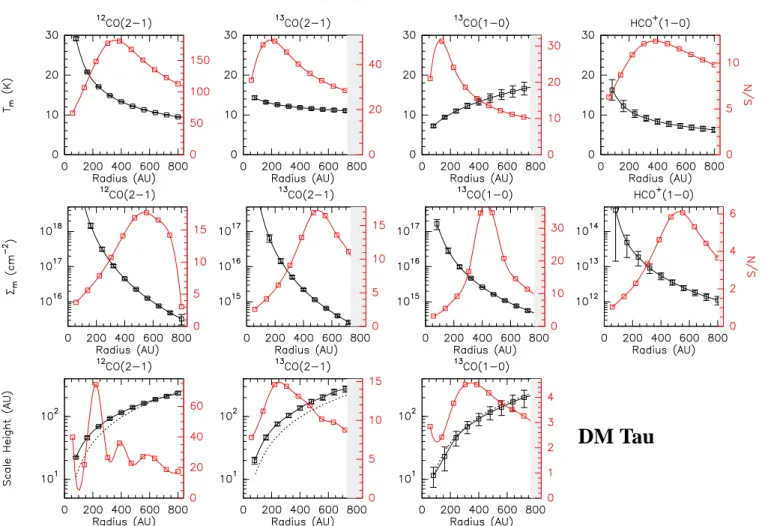
DM Tau
Fig. 4. From left to right12
CO J=2→1,13
CO J=2→1,13
CO J=1→0 and HCO+
J=1→0 in DM Tau. Top: Temperature Tm
(black curve, left axis) and signal to noise on the temperature Tm/δTm(grey curve, right axis) as a function of reference radius
RT.Middle Surface density Σm(left axis) and signal to noise on the surface density Σm/δΣm(right axis) as a function of reference
radius RΣ. Bottom Scale height h (left axis) and signal to noise on the scale height h/δh (right axis) as a function of reference
radius Rh.
weighting (Guilloteau & Dutrey 1998). We have implemented a modified Levenberg-Marquardt minimization scheme to search for the minimum, and we use the Hessian to derive the error bars. This scheme is much faster than the grid search technique used previously, and less prone to local minima. It allows to fit simultaneously more parameters, and thus provide a better es-timates of the errors because the coupling between parameters is taken into account.
However, the current fit method does not handle asymmet-ric error bars which happen in skewed distributions: this limi-tation should not be ignored when considering the errors on Σ,
T or Rout. The quoted error bars include thermal noise only, but
do not include calibration errors (in phase and in amplitude). Amplitude calibration errors will directly affect the absolute values of the temperature or the surface density (as a scaling factor, but not the exponent) while phase errors can introduce a seeing effect. The latter effect is very small for line analysis because molecular disks are large enough but it starts to be sig-nificant for dust disks. Our careful calibration procedure brings the amplitude effect to below 10 %. All other parameters are essentially unaffected by calibration errors.
3.3.2. Continuum Handling
The speed improvement allowed us to treat more properly the continuum emission. Even though the continuum brightness is small compared to the line brightness, continuum emission cannot be ignored when trying to retrieve parameters from the line emission because it appears systematically in all spectral channels.
A simultaneous fit of the continuum emission with its own physical parameters will properly take into account these bi-ases. We performed this by adding to the spectral UV table a channel dedicated to the continuum emission. The global χ2is given by the sum χ2= χ2
C+ χ 2 Lwhere χ 2 Cand χ 2 Lare the χ 2for
the continuum and for the line minimization, respectively. The continuum emission is fitted using the following parameters:
RCint, RCout, the inner and outer radii of the dust distribution, Σd
and pd, the surface density power law, and Tdand qd, the dust
temperature power law. Note that the representation of the con-tinuum needs only be adequate within the noise provided by the spectral (total) line width, about 10 to 20 MHz, rather than for the whole receiver bandwidth (600 MHz). A simplified model is thus often acceptable, as shown below.
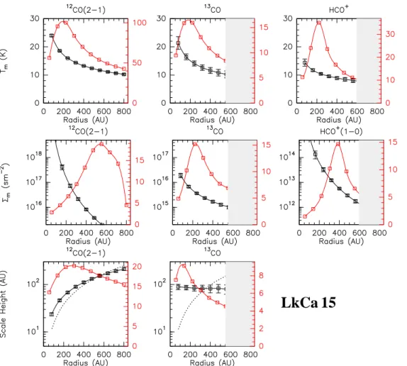
LkCa 15
Fig. 5. From left to right12CO,13CO and HCO+
J=1→0 in LkCa 15. Top: Temperature Tm(black curve, left axis) and signal
to noise on the temperature Tm/δTm(grey curve, right axis) as a function of reference radius RT.Middle Surface density Σm(left
axis) and signal to noise on the surface density Σm/δΣm(right axis) as a function of reference radius RΣ. Bottom Scale height h
(left axis) and signal to noise on the scale height h/δh (right axis) as a function of reference radius Rh. For HCO+ the temperature
and surface density were adjusted separately: the curves should be used as an indicator of the region over which these values are actually constrained, but not as a quantitative measure in terms of S/N, as the coupling between temperature and surface density is ignored.
We also compared this robust method with a simplified (and faster) one in which we subtract, inside the UV plane, the con-tinuum emission from the line emission before fitting. This sub-traction is not perfect: for the optically thick regions (which always occupy some fraction of the line emission) continuum should not be subtracted. However, unless the disk is seen face on, because of the Keplerian shear, at each velocity, the line emitting/absorbing region only occupies a small fraction of the disk area. This fraction is at most of order of the ratio of the local line width to the projected rotation velocity at the disk edge, in practice less than 10 – 15 % for the disks we con-sidered. Accordingly, the error made by subtracting the whole continuum emission in every channel is quite small.
We verified that this simplified method gives, as expected, the same results as the robust one. We used it, as it is signif-icantly faster. This better handling of the continuum allowed us to improve on the mass determination of MWC 480 (Simon et al. 2000), where the continuum is relatively strong.
3.3.3. Multi-Line fitting
The code has also been adapted to allow minimization of more than one data set at a time. This has been used to simultane-ously fit the13
CO J=1→0 and J=2→1 transitions. For multi-line fitting, the temperature is derived from the multi-line ratio. The temperature is determined in the disk region where both lines are optically thin. In this case, the fit is much more accurate than from a single line observation if there is no significant vertical temperature gradient. When a temperature gradient is present, the derived temperature will reflect an “average” tem-perature weighted by the thermal noise.
4. Results
4.1. Interpretation of the Power Law model
The parametric model would perfectly describe the line emis-sion from a molecule in LTE in a vertically isothermal disk which is in hydrostatic equilibrium, with power law for the ki-netic temperature and surface density, and constant molecular
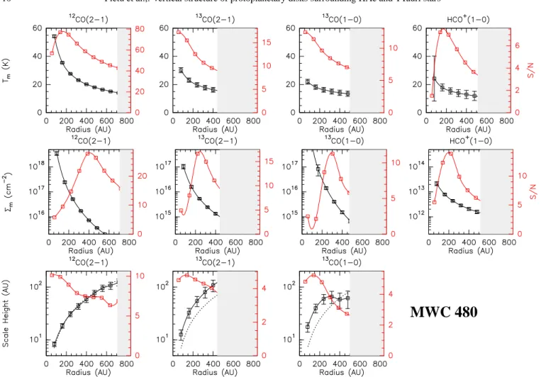
MWC 480
Fig. 6. From left to right12
CO J=2→1,13
CO J=2→1,13
CO J=1→0 and HCO+
J=1→0 in MWC 480. Top: Temperature Tm
(black curve, left axis) and signal to noise on the temperature Tm/δTm(grey curve, right axis) as a function of reference radius
RT.Middle Surface density Σm(left axis) and signal to noise on the surface density Σm/δΣm(right axis) as a function of reference
radius RΣ. Bottom Scale height h (left axis) and signal to noise on the scale height h/δh (right axis) as a function of reference
radius Rh. As for LkCa 15, temperature and surface density are adjusted separately for HCO+.
abundance. In such a case, ev = q/2 if the local line width is
thermal, and h = q/2 − 1 − v and h0 = ( p
2kT0/m)/V0
(us-ing the same reference radius Rh = RT = Rv, m being the
mean molecular weight). If such a disk was chemically ho-mogeneous, all molecular lines would yield the same results for the 17 parameters (after correction of Σmfor the molecule
abundance). Differences between the parameters derived from several transitions will reflect departures from such an ideal sit-uation.
For example, the geometric parameters PA and i should all be identical, as should be the kinematic parameters Vdisk,V0,v
(and we should have v = 0.50 for Keplerian rotation). X0,Y0
should reflect the absolute astrometric accuracy of the IRAM interferometer. Different values for Tmfrom several transitions
for the same molecule, or its isotopologues, may reveal vertical temperature gradients, or, in case of non-LTE excitation, den-sity gradients, since such transitions probe different regions of the disk. The values of Tmfrom different molecules may also
provide constraints on the density, because of the different crit-ical densities. And, more directly, the values of Σm, pm, Rinand
Rout will reflect the chemical composition of the disk as
func-tion of radius.
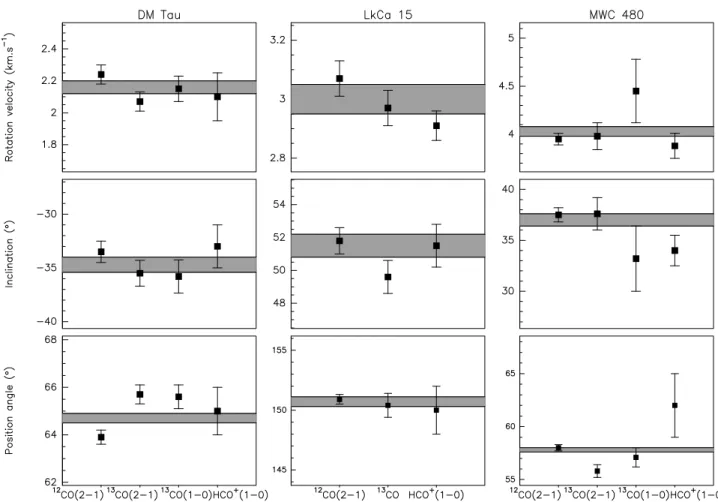
4.2. Geometric and kinematic parameters
Figure 7 shows the geometric and kinematic parameters PA,
i and rotation velocity V100derived from the observed
transi-tions in DM Tau, LkCa 15 and MWC 480. The grey area repre-sent the 1 σ range of the mean value computed from the CO lines. As expected, the derived value are in very good agree-ment altogether. In particular, the distribution of the derived values and the error bars are consistent with a statistical scat-tering, meaning that: i) the observed lines come from the same disk, ii) the error bars have the good magnitude, and iii) there is no bias in the determination of the parameters. This analysis of the “basic” parameters is of prime interest, because it shows that the analysis method is robust, and that the error bars have a real physical meaning. Although noisier, the kinematic and ge-ometric parameters determined from HCO+ are in agreement
with those found from CO. We thus used the CO-derived val-ues to determine the surface density and excitation temperature of HCO+.
Fig. 7. From left to right: kinetic and geometric parameters derived for DM Tau, LkCa 15 and MWC 480. From top to bottom: rotation velocity at 100 AU, inclination and position angle. For DM Tau and MWC 480, the error bars represent (from left to right) the value of the parameter measured from the12
CO J=2→1,13
CO J=2→1,13
CO J=1→0 and HCO+
J=1→0 lines. For LkCa 15 (from left to right), the values are derived from the12
CO J=2→1 line, from the simultaneous fit of the13
CO J=2→1 and the13
CO J=1→0 lines, and from the HCO+
J=1→0 line. In all three sources, the grey area represent ±1σ around the mean of the values of the CO isotopes.
4.3. Results
Tables 3, 4 and 5, present the best fit results for DM Tau, LkCa 15 and MWC 480, respectively. Compared to previous papers (e.g. Simon et al. 2000; Duvert et al. 2000; Dutrey et al. 1998), the new fits include all the refinements of the method described in Sec.3 and in Pi´etu et al. (2006).
All quoted results where obtained using cylindrical co-ordinates and the continuum was subtracted to the spectro-scopic data before analysis. All the models were obtained in the same manner. In particular, we assumed a constant line width (ev = 0), Keplerian rotation (v = 0.5), and a flaring
exponent eh = −1.25 (the value for a Keplerian disk in
hydro-static equilibrium with a temperature radial dependence of 0.5). This value is very close to those found by Chiang & Goldreich (1997) for the super heated layer model. Systematic tests with different sets of free parameters ensure that the geometrical and kinematical parameters are insensitive to these assumptions. The temperature Tm(r) is also hardly affected. The surface
den-sity Σm(r) and outer radius Routdepends to some extent on the
assumed flaring parameter eh. However, because of the
cou-pling between scale height and line width, both H0 and dV
should be taken with some caution. The dynamical mass
de-rived from 12CO also depends weakly on the assumed scale
height, since we derive the inclinations from the apparent CO surface.
The differences between the values reported here for DM Tau and those published by Dartois et al. (2003) come from the different assumptions in the analysis. Dartois et al. (2003) assumed hydrostatic equilibrium, and model the line width fol-lowing Eq.6 . They also assumed [12CO]/[13CO] = 60.
The 13CO emission in MWC 480 is strong enough to
al-low separate fitting of the J=2→1 and J=1→0 lines. We thus present separate results for each line. We also present a result in which both lines are fitted together: as expected in this case, the derived temperature is in between the results from the J=2→1 and J=1→0 transitions. However, for LkCa 15, the13CO emis-sion is too weak for a separate analysis: only the results from the simultaneous fitting of both13CO lines is presented.
For HCO+ in MWC 480, the signal to noise did not allow
an independent derivation of the temperature Tm: we used the
law derived from13CO. A similar problem occurs in LkCa 15:
for simplicity, we used Tm = 19 K and qm = 0.38,
solu-Table 3. Best parameters for DM Tau. (1) (2) (3) (4) (5) (6) Lines 12 CO J=2→1 13 CO J=2→1 13 CO J=1→0 Mean HCO+ J=1→0 Systemic velocity, VLSR(km.s−1) 6.026±0.002 6.031 ± 0.003 6.088 ± 0.004 6.038±0.002 6.01 ±0.01 Orientation, PA (◦) 63.9 ±0.3 65.7 ±0.4 65.6 ±0.5 64.7 ±0.2 65 ± 1 Inclination, i (◦) -33.5 ±1.0 -35.5 ±1.2 -35.8 ±1.5 -34.7 ±0.7 −33 ± 2 Velocity law: V(r) = V100( r 100 AU)−v Velocity at 100 AU, V100(km.s−1) 2.24 ±0.06 2.07 ±0.06 2.15 ±0.08 2.16 ± 0.04 2.10 ± 0.15 Stellar mass, M∗( M⊙) 0.56 ±0.03 0.48 ±0.03 0.52 ± 0.04 0.53±0.02 0.5 ± 0.1 Surface Density at 300 AU, (cm−2) 1.4 ± 0.6 1017
5.3 ± 1.1 1015
5.9 ± 0.6 1015
1.1 ± 0.3 1013
Exponent p 3.8 ± 0.3 3.4 ± 0.4 2.8 ± 0.3 2.3 ± 0.4
Outer radius Rout, (AU) 890 ± 7 720 ± 19 760 ± 22 800 ± 30
Temperature at 100 AU, (K) 26.0 ± 0.5 14.5 ± 0.5 8.0 ± 0.3 14 ± 2
Exponent q 0.49 ± 0.01 0.12 ± 0.03 −0.34 ± 0.07 0.40 ± 0.1
dV (km.s−1) 0.12 ± 0.01 0.15 ± 0.01 0.20 ± 0.01 0.13 ± 0.01
Scale Height at 100 AU, (AU) 30 ± 1.1 28 ± 4 28 ± 5 (19 ± 8)
Column (1) contains the parameter name. Columns (2,3,4) indicate the parameters derived from12
CO J=2→1,13
CO J=2→1 and13
CO J=1→0 respectively. Only12CO constrain the size of the inclination. Column (5) indicates the mean value of the kinematic and geometric parameters. Column (6) indicate the parameters derived from HCO+
J=1→0, obtained using a fixed inclination, orientation and stellar mass. For HCO+,
because of the lower resolution, the error on the temperature and surface density include contributions from the uncertainty on the exponent.
Tmis better constrained at 300 AU (9.0 ± 0.5 K), and Σmat 500 AU (3.2 ± 0.5 1012cm−2) .
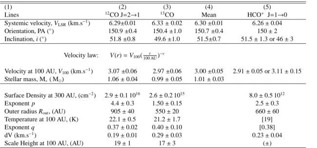
Table 4. Best parameters for LkCa 15
(1) (2) (3) (4) (5) Lines 12 CO J=2→1 13CO Mean HCO+ J=1→0 Systemic velocity, VLSR(km.s−1) 6.29±0.01 6.33 ± 0.02 6.30 ±0.01 6.26 ± 0.04 Orientation, PA (◦) 150.9 ±0.4 150.4 ±1.0 150.7 ±0.4 150 ± 2 Inclination, i (◦) 51.8 ±0.8 49.6 ±1.0 51.5±0.7 51.5 ± 1.3 or 46 ± 3 Velocity law: V(r) = V100( r 100 AU)−v Velocity at 100 AU, V100(km.s−1) 3.07 ±0.06 2.97 ±0.06 3.00 ±0.05 2.91 ± 0.05 or 3.11 ± 0.15 Stellar mass, M∗( M⊙) 1.06 ± 0.04 0.99 ± 0.05 1.01 ± 0.03 Surface Density at 300 AU, (cm−2) 2.9 ± 0.1 1016
2.6 ± 0.2 1015
8.0 ± 0.5 1012
Exponent p 4.4 ± 0.3 1.50 ± 0.15 2.5 ± 0.3
Outer radius Rout, (AU) 905 ± 40 550 ± 20 660 ± 60
Temperature at 100 AU, (K) 22.1 ± 0.5 21.2 ± 1.7 [19]
Exponent q 0.37 ± 0.02 0.40 ± 0.10 [0.38]
dV (km.s−1) 0.19 ± 0.01 0.29 ± 0.03 0.23 ± 0.04
Scale Height at 100 AU, (AU) 19 ± 1 17 ± 3 (±)
Column (1) contains the parameter name. Columns (2,3) indicate the parameters derived from12
CO J=2→1, and a combined fit of the 13
CO J=2→1 and13
CO J=1→0 respectively. Column (4) indicates the mean value of the kinematic and geometric parameters. Column (5) indicates the HCO+results: we used a fixed temperature law compatible with the CO isotopologue results (see text).
tion marginally better (1.7σ) with slightly lower temperatures (Tm= 13 K), with a somewhat steeper surface density gradient.
5. Discussion
We discuss here the physical implications of the results pre-sented in the preceding section. The following subsections fo-cus on the measurement of star masses, of the vertical tem-perature gradient, of the hydrostatic scale heights, of the CO abundances and CO outer radii, and of the HCO+distribution.
5.1. CO dynamical masses
Table 6 shows a comparison of the mass determination ob-tained in this work and in Simon et al. (2000). The subtrac-tion of the continuum has slightly improved the mass deter-mination in the case of MWC 480. Simon et al. (2000) used the old Solar metallicity (Z = 0.02) pre main-sequence (PMS) models. In Fig.8, we present here also results for a metal-licity Z = 0.01, much closer to the new Solar metalmetal-licity (0.0126, see Asplund et al. 2004; Grevesse et al. 2005, and references therein). LkCa 15 is in agreement with models of both metallicities (M = 0.95 ± 0.05 M⊙,t = 5 − 6 Myr and
Table 5. Best parameters for MWC 480. (1) (2) (3) (4) (5) (6) Lines 12 CO J=2→1 13 CO J=2→1 13 CO J=1→0 13CO HCO+ J=1→0 Systemic velocity, VLSR(km.s−1) 5.076±0.003 5.16 ± 0.02 5.17 ± 0.02 5.084 ± 0.003 5.11 ± 0.04 Orientation, PA (◦) 58.0 ±0.3 55.8 ±0.6 57.1 ±0.9 57.8±0.2 62 ± 3 Inclination, i (◦) 37.5 ±0.7 37.6 ±1.6 33.2 ±3.2 37.0 ±0.6 34.0 ± 1.5 Velocity law: V(r) = V100( r 100 AU)−v Velocity at 100 AU, V100(km.s−1) 3.95 ±0.06 3.98 ± 0.14 4.45 ±0.33 4.03± 0.05 3.88 ± 0.13 Stellar mass, M∗( M⊙) 1.76 ±0.06 1.65 ± 0.15 2.47±0.23 1.83± 0.05 1.70 ± 0.12 Surface Density at 300 AU, (cm−2) 3.6 ± 0.2 1016
3.3 ± 0.4 1015
5.3 ± 0.9 1015
4.5 ± 0.3 1015
3.4 ± 0.3 1012
Exponent p 4.7 ± 0.3 3.0 ± 0.4 4.5 ± 0.9 3.9 ± 0.3 1.5 ± 0.2
Outer radius Rout, (AU) 740 ± 15 450 ± 15 520 ± 70 480 ± 20 520 ± 50
Temperature at 100 AU, (K) 48 ± 1 28 ± 2 21 ± 4 23 ± 1 (15 ± 6)
Exponent q 0.65 ± 0.02 0.37 ± 0.08 0.28 ± 0.09 0.37 ± 0.04 (0.6 ± 0.4)
dV (km.s−1) 0.25 ± 0.01 0.25 ± 0.02 0.15 ± 0.03 0.21 ± 0.02 0.33 ± 0.07
Scale Height at 100 AU, (AU) 10 ± 1.1 18 ± 4 20 ± 2 19 ± 2
Column (1) contains the parameter name. Columns (2,3,4) indicate the parameters derived from12
CO J=2→1,13
CO J=2→1 and13
CO J=1→0 respectively. Column (5) indicates the mean value of the kinematic and geometric parameters (VLSR, PA, i, V100). For the other parameters, Column (5) indicate the results of a simultaneous fit of the two13CO transitions as for LkCa 15. Column (6) indicates the HCO+results: as the
temperature is poorly constrained, the surface densities were derived assuming the temperature given by13
CO J=1→0. The surface density is best determined at 250 AU: 4.3 ± 0.3 1012cm−2.
1.1 ± 0.1 M⊙,t = 4 − 6Myr, for Z = 0.01 and Z = 0.02
respec-tively). In fact, the measured dynamical mass does not provide any strong constraint on the location of LkCa 15 in this dia-gram (since the PMS tracks are almost parallel to the Y axis for stars with 0.5 < M∗/M⊙ < 1 in this distance independent HR diagram), but serves as a consistency check. However for MWC 480, either the metallicity is Z = 0.01 (i.e. nearly solar), in which case the derived dynamical mass is in agreement with the Siess et al. (2000) tracks (M = 1.8 M⊙,t = 8 Myr), or the
metallicity is 0.02 and MWC 480 would be located at a larger distance as suggested by Simon et al. (2000) (mass 1.9−2.0 M⊙,
age ∼ 7 Myr, and the distance would need to be increased by about 10 %)
Table 6. Stellar masses
Source Previous mass This work ( M⊙) ( M⊙) DM Tau 0.55 ± 0.03 0.53 ± 0.02 LkCa 15 0.97 ± 0.03 1.01 ± 0.03 MWC 480 1.65 ± 0.07 1.83 ± 0.05
See Simon et al., 2000 for the previous measurements. The old masses are based only on12CO while the new measurements are the average of all available CO lines.
5.2. Vertical Temperature Gradient
The primary goal of these observations was to confirm the find-ings of Dartois et al. (2003): the existence of a vertical temper-ature gradient. Fig.9 shows the tempertemper-atures deduced from the various CO lines versus the star effective temperatures in all sources of the sample. We confirm the DM Tau results with this slightly different analysis. MWC 480 also presents a significant
temperature difference between12CO and13CO. However, in
LkCa 15, there is no clear evidence of temperature gradient. As a general trend, the hotter stars of the sample, namely the Herbig Ae stars, exhibit larger kinetic temperature in the disks, not only at their surfaces but also for their interiors (see also Sect.5.8 for AB Aur). For MWC 480, even if the surface ap-pears hotter, a significant fraction of the disk (for r > 200 AU) remains at temperature below the CO freeze-out temperature.
The comparison between the three sources can be un-derstood by noting that the surface densities of 13CO
de-creases from DM Tau to MWC 480 and LkCa 15 (see Sect.5.8). Moreover, the temperature is lower in DM Tau, resulting in higher opacities for the J=2→1 and J=1→0 transitions than in the other sources. As a result, the location of the τ = 1 sur-face in the13CO lines differ in the three sources. In DM Tau, this surface is above (for the J=2→1 line) or at (for the J=1→0 line) the disk plane (as seen from the observer). A similar be-havior is observed in MWC 480.
In LkCa 15, the 13CO lines are nearly optically thin
throughout the disk, and the temperature is accurately deter-mined by the J=2→1/ J=1→0 line ratio. The lack of differ-ence between the12CO and13CO results indicate both lines are formed in a similar region: there must be little13CO at temper-atures much lower than indicated by12CO.
5.3. CO Surface density and outer radius
There are significant differences in surface densities between the three sources. At 300 AU, the measured surface densities of13
CO range from ∼ 2.5 1015 cm−2in LkCa 15 to ∼ 3.2 1015
cm−2in MWC 480 and ∼ 7 1015 cm−2in DM Tau. The
varia-tions are even larger for 12
CO with values ∼ 3 1016 cm−2 in
Fig. 8. Summary of the dynamical mass measurement for the sources of this sample. As in Simon et al. (2000), the results are shown in a distance corrected HR diagram (L/M2 versus T
e f f). New results have been obtained for MWC 480 and LkCa 15.
They are all compatible with the previous ones. In the case of MWC 480, the improvement in the mass determination is due to a better fit of the continuum, as explained in Sect.3.3.2. Left: Tracks for a stellar metallicity Z = 0.01. Right: Tracks for a stellar metallicity Z = 0.02. The models have been computed by Siess et al. (2000). Dots starts at 1 Myr and are spaced by 1 Myr. The tracks range from 0.5 to 2.0 by 0.1 M⊙, with the 2.2 and 2.5 M⊙tracks added. For Te f f, the error bars are assumed to be +/- one
sub spectral type class.
DM Tau (although the latter is uncertain by a factor 2 because of the steep density gradient).
The 12CO/13CO ratio is 20 ± 3 in DM Tau near 450 AU, the distance where this ratio is best determined. It is 11 ± 2 at 300 AU for LkCa 15, and 8 ± 2 for MWC 480. These values are much lower than the standard12C/13C ratio in the solar neigh-bourhood. These low values are most likely the result of sig-nificant fractionation, as in the Taurus molecular clouds, since the typical temperatures near 400 AU are around 12 K (see also Sect.5.8).
The exponent of the surface density distribution varies sig-nificantly. For DM Tau and MWC 480, an exponent of ∼ 3.5 is appropriate for all isotopologues. For LkCa 15, there is a large difference between the exponent for 13CO, 1.5, and that for 12CO, 4.5. Each line however samples a very different region
of the disk. The13CO data are most sensitive to the 200 – 300
AU region, while the12CO data is influenced by the outermost
parts, 500 – 700 AU (because of the opacity of the12CO line)
and up to the outer disk radius. The difference in exponent may thus indicate a steepening of the 12CO surface density distribution at radii larger than > 500 AU. At such radii, the
12CO emission becomes optically thin, and better constrains
the surface density than13CO. For DM Tau and MWC 480, the surface density of CO falls faster with radius than usually as-sumed for molecular disks (p ∼ 1 − 1.5, for H2). Note that
the uncertainty on temperature law affects only weakly the sur-face density derivation, specially for the J=2→1 transition for which the emission is essentially proportional to Σm for the
considered temperature range in the optically thin regime. This apparent steepening could reflect a change in the (H2) surface
density distribution in the disk. However, it can also be a result of chemical effects. The isotropic ambient UV field will tend to photo-dissociate CO isotopologues near the disk outer edge. Another effect is that, because of the lower temperatures,
de-pletion onto dust grains may be more effective at larger radii (although the lower densities result in a larger timescale for sticking onto grains).
Table 7. HCO+and CO Outer Radius
Source Rout(12CO) Rout(13CO) HCO+
(AU) (AU) (AU)
DM Tau 890 ± 7 740 ± 15 800 ± 80 LkCa 15 905 ± 40 550 ± 20 660 ± 60 MWC 480 740 ± 15 480 ± 20 520 ± 50
In all three sources, the outer radius in13CO is significantly
smaller than in12CO. In LkCa 15, the large difference may be
partly attributed to the change in the exponent of the density law. However, if we assume p = 1.5 for12CO, we get an outer
radius of 710 ± 10, still significantly larger than that for13CO.
The effect is thus genuine.
5.4. The LkCa 15 inner hole
In the case of LkCa 15, it is also important to mention its pe-culiar geometry: Pi´etu et al. (2006) have discovered a 50 AU cavity in the continuum emission from LkCa 15. We checked whether there is any hint of this cavity in the CO data. Adding the inner radius as an additional free parameter yields Rint =
13 ± 5 AU for12CO and R
int = 23 ± 8 AU for13CO. These
values are consistent with a smaller hole, or no hole at all, in CO and 13CO. The 50 AU inner radius determined from the
continuum is excluded at the 7 σ level in12CO, and at the 3 σ
level in13CO. Moreover the fit of a hole does not significantly
change the value of p, for both12CO and13CO emissions.
These small values indicate that the CO gas extends well into the continuum cavity. The cavity is thus not completely
Fig. 9. Temperatures derived from the CO isotopes versus ef-fective temperature of the central star. From left to right, the sources are DM Tau (filled triangles), GM Aur (empty stars), LkCa 15 (filled squares), MWC 480 (filled pentagons), HD 34282 (empty stars) and AB Aur (filled hexagons). From top to bottom,12CO J=2→1,13CO J=2→1,13CO J=1→0 temper-atures.
void, but still has a sufficient surface density for the 13CO
lines to be detected. The LkCa 15 situation is similar to that of AB Aur, for which the apparent inner radius increases from
12CO to13CO and to the dust emission (Pi´etu et al. 2005).
5.5. HCO+ surface density
The HCO+ data analysis reveal 4 major facts
– the outer radius in HCO+ is similar to that in12CO, and in
particular it is larger than that in13CO.
– in the two cases where it could be determined, the excita-tion temperature of the HCO+J=1→0 is lower than that of the13CO J=2→1 line.
– at 300 AU, the [13CO]/[HCO+] ratio is 500±150 (DM Tau), 320 ± 50 (LkCa 15), and 1300 ± 200 for MWC 480, with an additional uncertainty around 50 % for these last two sources due to the adopted temperature distribution. These values are similar to, although slightly smaller than the one found by Guilloteau et al. (1999) for the circumbinary disk of GG Tau (∼ 1500). On the other end, Pety et al. (2006) find a ratio of about 104 for the low mass disk around
HH 30, but at a smaller radius (100 AU).
– This ratio varies with radius: there is a tendency to have a somewhat flatter distribution of HCO+ than of CO (with
the exception of13CO in LkCa 15).
In DM Tau, the excitation temperature falls down to about 6 K beyond 600 AU, while the CO data indicates kinetic temper-ature of about 10 K in this region. Our calibration technique ensures that this is not an artifact. It may be a hint of very low temperatures in the disk mid-plane. On the other end, it may be an indication of sub-thermal excitation. However, as the criti-cal density for the HCO+
J=1→0 is only a few 104cm−3, such
a sub-thermal excitation would require that the HCO+ gas is
located well above the disk plane. Spatially resolved observa-tions of the HCO+ J=3→2 transition are required to check this possibility.
5.6. Turbulence in Outer Disks
We derive intrinsic (local) line widths ranging between 0.12 and 0.29 km.s−1. When taking into account the thermal compo-nent (0.08 to 0.15 km.s−1), from Eqs.6 and 7 we derive turbu-lent widths below 0.15 km.s−1. These values should be used as upper limits, since the spectral resolution used for the analysis (0.2 km.s−1) is comparable to the derived line widths. They are nevertheless significantly smaller than the sound speed,
Cs = 0.3 to 0.5 km.s−1in the relevant temperature and radius
range. The turbulence is thus largely subsonic. A more pre-cise analysis, using the full spectral resolution and an accurate knowledge of the kinetic temperature distribution, is required for a better determination.
5.7. Hydrostatic Scale Height
We follow the approach which is described in Sect.3.2.5 where the scale-height is not formally derived from the hydrostatic equilibrium. In a first step, the flaring exponent eh is taken
equal to eh = −1.25. Such a value is in agreement with
pre-dictions from models such as Chiang & Goldreich (1997) and D’Alessio et al. (1999). The observed transitions indicate ap-parent scale heights at 100 AU of 30 AU in DM Tau, and 19 AU in LkCa 15 and MWC 480 (see Tab.3-5). The only discrepant result is the value derived from12CO in MWC 480, 10 AU. In
a second step, treating ehas a free parameter provides similar
results, except for LkCa 15 where the13CO data is best fitted
by a flat (eh= 0), but thick disk (see Fig.5).
On the other end, using the temperature derived from the
13
CO J=2→1 transition as appropriate, we can derive the hy-drostatic scales heights. These scale heights are 15, 13 and 9.5 AU, respectively for DM Tau, LkCa 15 and MWC 480, with a typical exponent eh = −1.35, approximately 1.5 – 2 times
smaller than the apparent values. Although, as mentioned in Sect.3.2.5, the scale height has to be interpreted with some caution (especially when determined from12CO), these results suggest that CO has a broader vertical distribution than what is expected from an hydrostatic distribution of the gas. The cur-rent data do not allow us to identify the causes of this effect. Vertical spreading due to turbulence can be rejected as the tur-bulence is largely subsonic (see Sect.5.6). The larger apparent height may be due to CO being more abundant in the photo-dissociation layer above the disk plane.
5.8. Comparison with other Disks and Models
Only one other source has been studied at the same level in the CO isotopologues: AB Aur by Pi´etu et al. (2005). The temperature behavior of the AB Aur disk is similar to that of the MWC 480 disk, although the AB Aur disk is warmer. Temperature derived from CO for all sources are summarized in Fig.9. As expected, the disk temperatures (midplane and