Stochastic simulation of channelized sedimentary bodies using a constrained L-system

(1)

Stochastic

simulation of channelized sedimentary bodies using a

constrained

L-system

Guillaume

Rongier

a,b,⁎

,

Pauline Collon

a

,

Philippe Renard

b

a _{GeoRessources}_{(UMR 7359, Université de Lorraine / CNRS / CREGU), Vandœuvre-lès-Nancy F-54518 France} b _{Centre d′Hydrogéologie et de Géothermie, Université de Neuchâtel, 11 rue Emile-Argand, Neuchâtel 2000, Switzerland}

Keywords: Sedimentary system Channel Stochastic simulation Lindenmayer system Data conditioning Constraints

A B S T R A C T

Simulating realistic sedimentary bodies while conditioning all the available data is a major topic of research. We present a new method to simulate the channel morphologies resulting from the deposition processes. It relies on a formal grammar system, the Lindenmayer system, or L-system. The L-system puts together channel segments based on user-deﬁned rules and parameters. The succession of segments is then interpreted to generate non-rational uniform B-splines representing straight to meandering channels. Constraints attract or repulse the channel from the data during the channel development. They enable to condition various data types, from well data to probability cubes or a conﬁnement. The application to a synthetic case highlights the method's ability to manage various data while preserving at best the channel morphology.

Introduction

The presence of channelized sedimentary bodies constitutes a key structuring element for the connectivity of a reservoir. These bodies are composed of heterogeneous deposits that can containfluids or act as flow barriers. Such barriers may compartmentalize the reservoir and make its exploitation harder, especially when combined with sealing faultsGainski et al. (2010). Channel modeling can help to study and anticipate more precisely the flow behavior. It requires a balance between geological concepts and data conditioning, which remains an issue in stochastic simulation.

Stochastic simulation methods are usually split in two categories: cell-based and object-cell-based methods. Cell-cell-based methods (e.g.,Deutsch and Journel, 1992; Galli et al., 1994; Strebelle, 2002) attribute a sedimentary body type– e.g., channel – to each cell within a grid, based on a prior model. It makes well data conditioning easy, but the channel continuity is rarely preserved. The resulting connectivity differs from the prior model or from object-based methods (Rongier et al., 2016). Object-based methods (e.g., Viseur, 2001; Deutsch and Tran, 2002; Pyrcz et al., 2009) rely on a geometrical representation of the channels, with para-meters such as their width or their wavelength. They preserve the channel continuity. However, data conditioning is difficult, because of the elongated shape of channels and the poorflexibility of their representa-tions.

In numerical biology, tree and root simulation also relies on object-based approaches (e.g.,Prusinkiewicz and Lindenmayer, 1996; Leitner

et al., 2010; Longay et al., 2012). A formal grammar– the Lindenmayer system or L-system (Lindenmayer, 1968)– mimics tree and root growth to simulate the related objects. An interesting development of such methods introduces the environment influence to improve the simulation realism: influence of gravity, influence of the sun light distribution, influence of other trees, etc. (e.g., Mvech and Prusinkiewicz, 1996; Streit et al., 2005; Taylor-Hell, 2005). Despite this ability to integrate various data, very few works use formal grammars to simulate channels.

Hill and Griﬃths (2009)rely on an analog model to deﬁne some rules for channel stochastic simulation, with a conditioning limited to well data or channel segments interpreted on seismic data.

In this paper, we present a new method to simulate channels based on L-systems. L-system rules control the channel morphology to simulate straight to sinuous channels (Section 1). During the simula-tion, constraints inﬂuence the channel growth to condition various data (Section 2). The purpose of this research is to facilitate data condition-ing as compared to other object-based approaches while keepcondition-ing their main added-value: the preservation of the channel shape. A synthetic case study applies the method to the simulation of submarine channels within an incised valley (Section 3). It leads to a discussion on the channel simulation with L-system and constraints (Section 4). 1. L-system for channel stochastic simulation

This object-based method relies on a L-system to give form to a parameterized channel geometry.

⁎_{Corresponding author at: GeoRessources (UMR 7359, Université de Lorraine / CNRS / CREGU), Vandœuvre-lès-Nancy, F-54518 France.} E-mail address:guillaume.rongier@univ-lorraine.fr(G. Rongier).

(2)

1.1. Channel object deﬁnition and simulation principle

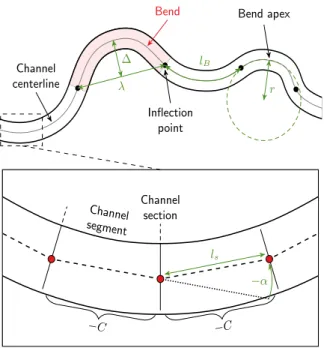
A channel object is built upon Non-Uniform Rational B-Splines (NURBS)– a generalization of Bézier curves (Piegl and Tiller, 1995)– as deﬁned byRuiu et al. (2015). In this model, a channel appears as a discretized object composed of channel segments separated by trans-versal channel sections (Fig. 1). A section is at the end of its respective segment. An orientation and a distance from the previous section characterize a given section.

A L-system builds the succession of sections and determines their location. A sequential Gaussian simulation (Deutsch and Journel, 1992) simulates a width and thickness for each channel section, with a possible inﬂuence of the channel curvature. The section locations, widths and thicknesses are the foundation for the NURBS representa-tion. This method is designed for a classical modeling workﬂow, which consists in building a geological grid from a structural model, and simulating the channels inside the parametric space of this grid (Dubrule et al., 1997).

1.2. Brief introduction to L-systems

The Lindenmayer system is a formal grammar designed by

Lindenmayer (1968) to simulate the development of ﬁlamentous organisms. Since then, it has been expanded to simulate the develop-ment of plants (e.g., Mvech and Prusinkiewicz, 1996; Prusinkiewicz et al., 2001; Leitner et al., 2010). A L-system aims at rewriting an initial string, the axiom, with production rules, all composed of letters from a predeﬁned alphabet. The rules include a set of letters to replace, the predecessor (pred), and a set of replacement letters, the successor (succ):

lc<pred param( ) > :rc cond→p succ param( ′)

The application of a rule may depend on the letters before and after the predecessor, called respectively the left and right context (lc and rc), on a probability (p), and on parameters (param and param′) and condi-tions (cond). The following example contains an axiomω and three production rules p1, p2, and p3:

ω b p a h b h b h p a h b h a h a h p b h h a h b h : (0) : ( ) > ( ) ⟶ ( + 1) : ( ) > ( ) ⟶ ( ) ( ) : ( ) : < 1 ⟶ ( ) ( ) 1 0.75 2 0.25 3

The rules may rewrite the axiom as follows:

μ b ω μ a b p μ b a b p p μ b a a a b p p : (0) ( ) : (0) (0) ( ) : (1) (0) (0) ( & ) : (1) (0) (0) (0) (0) ( & ) 0 1 3 2 1 3 3 2 3

The resulting string constitutes a sequence of commands, which control an interpreter called a turtle (Prusinkiewicz, 1986). The turtle's state is represented by a position vector P⎯→⎯ and an orthonormal coordinate system centered on this position, with:

•

_{H the forward direction.}l

•

l_L_{the left direction.}

•

_{U the up direction.}l

This state is built from an initial position and orientation. Then, the letters update it and draw object elements, such as segments, along the way to progressively build the object. More details about L-systems can be found inPrusinkiewicz and Lindenmayer (1996).

1.3. Alphabet for channel simulation

A channel is decomposed into bends separated by inﬂection points (Fig. 1). A bend is a succession of channel segments whose orientations change along the same direction. Seven letters constitute the alphabet to model this succession of segments (Table 1).

A channel divides into two branches that grow in opposite direc-tions. Brackets [and] symbolize this branching structure, with the letters of thefirst branch in between. The letter C builds the channel object, while the letters + and - control the channel sinuosity. A channel segment is symbolized by a ± C pair. Thus, a channel is a succession of ± C letters, with ± being + or− but remaining the same along the bend. The letter I has no influence on the string rewriting. It only states the initial position during the geometrical interpretation. The letter T has no influence on the geometrical interpretation. It only ensures the channel growth during the rewriting.

1.4. Production rule deﬁnition

The rules aim at building bends from channel segments. This includes converting the input parameters that describe the channel morphology into L-system parameters.

Fig. 1. Channel discretization for L-system simulation. The red dots locate the channel sections obtained from the interpretation. lsis the distance between two successive sections, i.e., the channel segment length.α is the angle between two successive sections, i.e., the change of orientation between two successive channel segments. The other parameters characterize a channel bend, with lBthe bend length,λ the bend half-wavelength,Δ the bend amplitude, and r= 1/ the radius of curvature – radius of a circlec ﬁtted at the bend apex – with c the curvature.

Table 1

L-system alphabet for channel simulation. Letters (parameters) Interpretation

I First letter of a L-system string that contains the initial position

T Do nothing

C l( )s Move forward of a length lsand draw a channel segment between the new position and the former one α

+( ) Turn left by an angleα α

−( ) Turn right by an angleα

[ Start a branch, i.e., push the current turtle's state into a stack

] End a branch, i.e, pop a state from the stack to be the current turtle's state

(3)

1.4.1. From input to L-system parameters Simulating the channel morphology calls for:

•

The global direction lD along which the channel must be oriented.

•

The default length ld for the channel segments to deﬁne the

discretization resolution.

•

The bend half-wavelengthλ and the bend amplitude Δ (Fig. 1) to deﬁne the bend morphology. They are drawn from statistical distributions for each new bend.

•

The deviation angle δ to perturb the bend morphology, because a half-wavelength and an amplitude are not enough to characterize a bend (Howard and Hemberger, 1991). It is drawn from a statistical distribution for each new channel segment.

The bend length and the curvature can replace the bend half-wavelength, the bend amplitude and the deviation angle (Rongier, 2016).1_{The purpose is then to retrieve the two L-system parameters l}

s

andα.

It starts by determining the curvature c with the intersecting chord theorem and the law of cosines:

c Δ

Δ λ

= 8

4 2+ 2 ₍₁₎

c provides the bend length lB, i.e., the curvilinear distance between two

inﬂection points (Fig. 1):

l c

c

= 2arccos(1 − Δ )

B ₍₂₎

lBand lddetermine the number nsof bend segments:

ns= ⌈ / ⌉l lB d (3)

where x⌈ ⌉ rounds x upward. The segment length lsbecomes:

l_s= /l n_B _s (4)

Finally, the angleα between two successive segmentsi− 1and i comes from the curvature and the lengths of both segments, perturbed by the deviation angle:

α= c l( + )l δ

2 +

s i, −1 s i,

(5)

1.4.2. Rules for channel simulation

The channel initial position is randomly drawn inside the geological grid, possibly inﬂuenced by a grid property. The initiation rules simulate a single bend separated into the two branches (Fig. 2). The numbers of segments for each branch, ns₁and ns₂, are computed by:

< n n n n n ∼ (1, − 1) = − s s s s s 1 2 1 (6)

with ns the number of bend segments and < a uniform discrete

distribution deﬁne by its minimal and maximal values. ns₁is randomly

drawn from this distribution. Instead of using Eq.(5), the anglesα1and

α2 of the ﬁrst segment of each branch are modiﬁed into to initially

orient the channel along the global direction:

α α n α α n α cl δ = × ( − + 1) = × ( − ) = + n s n s s 1 0 ₂ 2 0 2 0 s s 1 2 (7) whereδ is the deviation angle, c is the curvature (Eq.(1)), and lsis the

segment length (Eq.(4)). The initiation rules are stochastic, with two rules for the two possible bend orientations. A letter T at each branch extremity enables further growth.

The channel growth is ensured by the development rules, which tie bends one after the other. These rules replace a T by a new bend depending on the left context, and add a T at the end to pursue the channel development (Fig. 2). This enables to change the orientation from one bend to the other. The process stops as soon as the two branches go outside the geological grid. The simulation can also stop at a given channel length. The complete rules for channel simulation are available inRongier (2016). These rules are predeﬁned, but nothing

prevents from modifying them.

1.5. Extending the inﬂuence of the global direction

Only theﬁrst segment of each branch aligns the channel along the global direction (Eq.(7)). When the L-system parameters do not vary much between bends, the channel keeps following the channel direc-tion. When the L-system alternates straight and sinuous bends, the channel diverts from the global direction and often self-intersects. Those potential inconsistencies result from the L-system interpretation principle: a new segment only knows its immediate previous neighbor. Extending the inﬂuence of the global direction to the whole system better controls the channel orientation and limits self-intersections. It occurs after the orientation change of the letters + and -. The global direction lD reorients the turtle's head lH :

m l l H K K K H o D ′ = ⎯→⎯ ∥⎯→⎯ ∥ ⎯→⎯ _{= ϵ} _{+ ϵ} h d (8)

withmH′the new turtle's head,ϵha weight on the L-system,ϵda weight

on the global direction and o the branch orientation, equal to 1 for one branch and−1 for the opposite branch. ϵhandϵdare user-deﬁned, and

control the inﬂuence of the L-system and the global direction. 2. Constraints for data conditioning

In biology, constraints make trees interact with their environment (e.g., Taylor-Hell, 2005; Longay et al., 2012). Here, constraints condition the data.

2.1. Formalization

An environmentally-sensitive process adds the constraints to the L-system. After each rewriting step, an interpretation deﬁnes the spatial relationship between the channel and its potential constraining ele-ments. The constraints are separated into:

•

Relative constraints, whose magnitude depends on the distance to their constraining element.

•

Global constraints, whose magnitude is independent from a con-straining element.

A constraint is also attractive or repulsive (Fig. 3).

Building constraints means choosing one or several constraining elements within a perception area (Fig. 4) and determining the constraint vectors. These vectors indicate where the system should go under the constraint inﬂuence. They decompose into three elements:

•

The constraint direction lΛ , de_{ﬁned from the vector}V→between the turtle's head and a point on the constraining element, either its center or the closest location to the turtle's head. (Fig. 3):

l l l ⎧ ⎨ ⎪⎪ ⎩ ⎪⎪ Λ =

if the constraint is attractive if the constraint is repulsive

V V D V D V → ∥→∥ −→ ∥ −→∥ (9)

(4)

with lD the global channel direction.

•

The constraint magnitudeρ. It is equal to one for a global constraint, and depends on the distance to the constraining element for a relative constraint (Fig. 5).

•

A user-deﬁned weight ϵ to adjust the relative importance of each constraint.

2.2. Examples of constraining data

Wells provide local and often precise data about facies and sedimentary bodies. We consider two types of well data (Table 2):

•

Channel data comes from channelized bodies. A channel is attracted by one channel datum at a time until conditioning, i.e., the datum ends up in a channel.

•

Inter-channel data correspond to other sedimentary bodies around channels, such as levees. A channel is repulsed by inter-channel data, i.e., these data must never end up in a channel.

Seismic data provide an overview of the underground in three-dimensions. We consider two constraints from seismic data (Table 2):

•

With enough resolution, seismic data can help interpret the channel

conﬁnement (e.g.,Allen, 1982; Janocko et al., 2013), a major source of uncertainty (Larue and Hovadik, 2008). Here a geological grid materializes the conﬁnement and constraints prevent the channels from going out (Table 2).

•

With a low resolution, a sand probability cube can be extracted (e.g.,

Strebelle et al., 2003). As channels often have a sandyﬁlling, the high sand probabilities attract the channels (Table 2). The mean of many realizations (the E-map) should come close to the probability cube, without forgetting that simulating channels is not simulating sand distributions.

2.3. Adding the constraints to the L-system

Once deﬁned, the constraints are added to the turtle head lH :

m l l l l H K ρ H ρ D ρ Λ ρ Λ ρ ρ ′ = = ϵ + ϵ + ∑ ϵ + ∑ ϵ = ∏ (1−ϵ ) K K h r d r j n g j r j i n r i i i r i n r i i ⎯ →⎯⎯ =1 , =1 , =1 , g r r ⎯→⎯⎯ ⎯→⎯⎯ (10) withmH_′the new turtle head, ngthe number of global constraints and nr

the number of relative constraints.ϵg j, is a user-deﬁned weight for each

Fig. 2. Simplified illustration of channel simulation with a L-system. The red point is the initiation point. The first iteration stochastically initiates the two channel branches. The following iterations grow the channel. Unless otherwise specified, + and − stand for+( ) andα −( ) (see Eq.α (5)), and C for C l( )s (see Eq.(4)).α1andα2come from Eq.(7).

(5)

global constraint j. ϵr i, is a user-deﬁned weight for each relative

constraint i.ϵhandϵdare the user-deﬁned weights for the L-system

and the global direction.ρiis the magnitude of the constraint i and lΛi

the constraint direction. The magnitudeρrdecreases the turtle's head

magnitude, the global direction magnitude and the global constraint magnitudes when a relative constraint has a high magnitude. This improves the conditioning by limiting the inﬂuence of the other constraints when getting close to the considered data.

2.4. Constraint setting

Constraints call for numerous parameters, which limits their practicality. We have deﬁned default values for the data of Section 2.2(Rongier, 2016). For most cases, they should be suﬃcient to ensure the conditioning, and can be adjusted otherwise. Among all the parameters, ten are still required as input (Table 3) when constraining all these data.

Four parameters are the weightsϵ of the constraints to adjust their relative importance. The channel global direction is already required by the L-system. The channel minimal and maximal width and minimal thickness come from the distributions required by the L-system. The bandwidth for the well channel data is the only parameter with the constraint weights that is not shared with the L-system. It controls the lateral extension of the perception area and inﬂuences the well connections through the channels.

3. Application

The method was implemented in C++ in the Gocad plug-in ConnectO. The NURBS channel model was implemented by Jérémy Ruiu in the Gocad plug-in GoNURBS (Ruiu et al., 2015). This section develops an application to a synthetic case combining diﬀerent data. SeeRongier (2016)for applications to explore parameter and conditioning eﬀects.

3.1. Dataset

The synthetic case is build upon submarine channels that migrate within a conﬁning valley. Such channels often display two migration patterns (e.g.,McHargue et al., 2011):

Fig. 3. Constraint addition to a L-system, with lH the current turtle's head, mH′ the new turtle's head inﬂuenced by the constraint, lD the channel global direction, lΛatt the direction for an attractive constraint, deduced from V→, lΛrepthe direction for a repulsive constraint, deduced from V−→and lD , and V→the vector between the turtle's head and the constraining element.

Fig. 4. Parameters deﬁning the perception area, with ld its direction,σ its direction tolerance, waits maximal half-width, laits length and taits thickness. lH is the turtle's head.

Fig. 5. Parameters controlling the magnitude of a relative constraint: the distance dmax deﬁnes if the element is conditioned, the bend length lband the factors f1and f2adjust the constraint behavior, andτ1,τ2,τ3andτ4deﬁne the magnitude values.

Table 2

Constraints used inSection 3.

Constraint Type Element

Well channel data Relative & attractive Well point Well inter-channel data Relative & repulsive Well point Probability cube Global & attractive Grid cell Conﬁnement (margin 1) Relative & repulsive Grid border Conﬁnement (margin 2) Relative & repulsive Grid border

Table 3

Input parameters for the constraints ofSection 2.2, withϵithe constraints weights, tmin the minimal channel thickness, lD the channel global direction, wa CD, the perception area

bandwidth for the well channel data and wminand wmaxthe minimal and maximal channel widths.

Input parameters

Well channel data ϵCD Dl wa CD, wmin tmin Well inter-channel data ϵICD Dl – wmax tmin

Probability cube ϵPC Dl – – tmin

Conﬁnement (margin 1) ϵC Dl – wmax –

(6)

•

In the lower valley part, channels mostly migrate laterally, with some disorganized stacking between the channels due to discrete migration. This distributes the sandy deposits over the whole valley width.

•

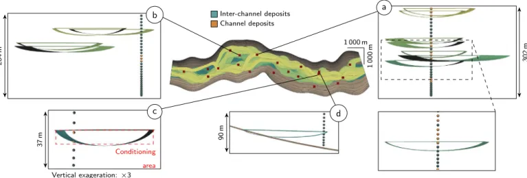
In the upper part, vertical migration dominates, with the develop-ment of overbanks that conﬁne the channels. The sandy deposits are localized over a smaller section of the valley.

The data set emulates these features through (Fig. 6):

•

A hexahedral grid aligned along its margins, simulated with a L-system and NURBS to materialize the valley.

•

A sand probability cube inside the valley grid, with high sand probabilities along the whole valley bottom and more localized at the top. It comes from a sequential Gaussian simulation conditioned to a property whose top derives from a channel simulated with a L-system and whose bottom is evenlyﬁlled.

•

234 channel and 391 inter-channel data points extracted along 20 random well paths from a realization conditioned to the sand probability.

The associated constraints are those from Table 2. Table A.1 sum-marizes the input parameters.

3.2. Simulation principle

Channels are simulated inside the grid parametric space as long as some well channel data remain unconditioned. Their initial position is drawn close to channel data. The L-system growth is then influenced by the confining valley, the sand probability cube, and the well data, but not by the previously simulated channels. Only an unconditioned channel datum can attract a channel. Once all the channel data are conditioned, channels are still simulated up to a target number of channels – here 40 – if not already reached. The initial position of these last channels is randomly drawn inside the grid. The probability cube influences this draw, so that channels appear preferentially in the high sand probability areas.

3.3. Simulation results

The simulated channels remain sinuous despite the signiﬁcant number of constraints (Fig. 7). The channel global direction skews the bends, similarly to the observations on real cases (Fig. 8). However, the bends are deformed depending on the constraint direction, which is not necessarily oriented along the global ﬂow direction. With a high global direction weight, the bends have opposite asymmetries on the two branches (Fig. 8). For now, no solution has been found to control the bend asymmetry.

(7)

The channel centerlines never go outside the valley, but sometimes the channel objects do. This often occurs when an inter-channel datum is too close to a margin: the two constraints may compete with each other, and the channel ends up violating both (Fig. 9, d). The channels honor all the channel data, as the simulation would not stop otherwise. But the conditioning area is based on a horizontal and a vertical distance: it is rectangular, not channel-shaped (Fig. 9, c). For the realization in Fig. 7, 15 over 234 channel data points are outside a channel and would require a post-process to strictly condition them. Similarly, some channels condition 30 over 391 inter-channel data. This is either a failure of the repulsive process (Fig. 9, b), or a channel that conditions both a channel and an inter-channel datum (Fig. 9, a). This last case arises because the simulation is meant to favor channel data conditioning: an inter-channel datum below the channel data to condition is ignored.

59,38 channels are simulated on average over 100 realizations, with a standard deviation of 3.64. No realization has less than 49 channels, far from the 40 channels required in input. And the well data come from a realization of 40 channels. The number of channels increases due to well channel data conditioning.

3.4. Eﬀect of the constraints

The constraints deform the channel morphology simulated by the Fig. 7. Realization conditioned to the sand probability cube and well sedimentary data within the conﬁning valley The highest channel – on the right – must remain inside the valley while following the high sand probability without conditioning the 14 inter-channel data and with 6 channel data that it may condition. The two channel data outside this channel condition another channel.

Fig. 8. Asymmetric bends on a seismic section from Angola (modiﬁed from Kolla et al. (2001)) and below a channel simulated with a L-system showing opposite bend asymmetries from the initiation point.

(8)

L-system to condition the data. E-maps of realizations with different constraints (Fig. 10) highlight this impact. With the current setting, the margins have a significant repulsive effect on the channels, preventing them from equally covering the entire valley (Fig. 10, a). This is why the

channels tend to gather along the center of the valley bottom, in contradiction with the sand probability cube (Figs. 6 and 10, b). However, the channels strictly follow the upper trend of the sand probability. The resulting E-map is less blurry than the sand prob-Fig. 9. Details on well conditioning. All the channels are not showed for clarity. a. The four channels at the top perfectly condition the channel data. In the middle, the last channel condition both a channel data and an channel data: currently the process can not always prevent the channel data conditioning. b. Five channels are close to a set of inter-channel data. One of them condition the inter-inter-channel data, showing a failure in the repulsion process. c. The inter-channel conditions the two inter-channel data as deﬁned in the method. However, the channel data at the bottom is not within the channel and is not stricto sensu conditioned. d. Example of incompatibility between the L-system path and the data.

(9)

ability, but the channelﬁlling should be simulated for further compar-ison. Adding well sedimentary data causes the channels to locally divert from the upper trend of the sand probability (Fig. 10, c). It exempliﬁes the constraint competition with two data sets that are not fully compatible. Here priority is given to well data, sometimes placing a lower emphasis on the sand probability cube.

A comparison with a conditioning by rejection sampling helps to further analyze the bias introduced by the constraints on the channel morphology (Fig. 11). The rejection sampling is a simplistic but unbiased conditioning process: an unconditional channel is simulated and kept if itﬁts the data. Otherwise, a new channel is simulated. Here the channel sections within the inter-well area appear slightly less variable with the constraint than with the rejection sampling. It comes from the straighter morphology of the channels due to the constraint. This bias could be reduced by adapting the constraint setting, especially the magnitude.

3.5. Simulation time

Simulating2_{channels in the con}_{ﬁning valley is quite fast (}_{Table 4}_).

Adding constraints impacts the computation time, but it remains acceptable for stochastic purposes. For the probability cube, the main time increase comes from the search for the constraining cell in the perception area. A small area length lalimits the computation time but

the conditioning becomes more sensitive to small scale variations. The time increase when adding well data mainly comes from the higher number of simulated channels to condition all the channel data. The NURBS generation is the most time consuming process.

The comparison with the simplistic rejection sampling ofFig. 11yet highlights the significant speed of the conditioning process by con-straints (Table 5). On average, the constraint is 100 times faster than the rejection sampling. And this case has fewer data than the confining valley case, in which the rejection sampling is not an option. The smaller computation times of the NURBS surfaces under the constraint influence come from the straighter channels.

4. Discussion and perspectives

The synthetic case illustrates the method ability to simulate channels while conditioning various and numerous data. This section discusses some aspects of the simulation process.

4.1. About the use of L-systems

Formal grammars remain uncommon in geological simulations, despite a successful use in other domains.Hill and Griﬃths (2009)use a diﬀerent kind of formal grammar to simulate channels: the plex grammar (Feder, 1971). In the L-system formalism, a letter has two

attaching points, with a letter to its left and one to its right. The plex grammar generalizes this principle to connections between an arbitrary number of letters. It better handles three-dimensional shapes, but the rules quickly become unwieldy.Hill and Griffiths (2009)bypass this issue by using a training model, from which the rules are inferred. Our approach complements it by simulating channels from scratch, avoid-ing a trainavoid-ing model that may be difficult to get. With predefined rules, the L-system itself does not require more parameters than other object-based approaches (e.g., Viseur, 2001; Deutsch and Tran, 2002; Hassanpour et al., 2013). The bend half-wavelength, bend amplitude and channel width can be inferred from seismic data, the channel thickness from well data (e.g.,Wonham et al., 2000). When the well data are too sparse or the seismic resolution too low, these parameters can come from seismic or outcrop data of analog settings (e.g.,

McHargue et al., 2011; Colombera et al., 2012).

One main advantage of L-systems or other formal grammars is the possibility to change the rules. Modifying the channel morphology or introducing non-stationarity along the channel path (Rongier, 2016) becomes easy once the formalism is known. This brings moreflexibility to the object definition than in other approaches (e.g.,Viseur, 2001; Deutsch and Tran, 2002; Hassanpour et al., 2013) and facilitates user interaction. It is one step toward dealing with one major drawback of object-based methods: the need for predefined geometry for the objects to simulate. Here focusing on the channel morphology helps to preserve the rule simplicity. Butfinding simple rules to simulate the whole three-dimensional shape of the channel could be a step forward to a more interactive modeling process, such as what is already done in Fig. 11. E-maps of 1000 realizations conditioned to two well channel data using two different conditioning processes. L-system weight: 1; global direction weight: 0.2 (rejection sampling). L-system weight: 1; global direction weight: 0.2; channel data weight: 1 (attractive constraint).

Table 4

Simulation time for a realization in the confining valley with different constraints. The given values are the average time over 100 realizations and the standard deviation.

Constraints L-system

simulation (in s)

NURBS generation (in s)

Conﬁnement only 3.17 ± 0.15 16.24 ± 0.22 Conﬁnement and probability

cube

4.73 ± 0.10 14.57 ± 0.15 Conﬁnement, probability

cube and well data

6.64 ± 0.45 21.47 ± 1.31

Table 5

Simulation time for a realization containing one channel with two different conditioning processes. The given values are the average time over 1000 realizations and the standard deviation.

Conditioning type L-system simulation (in s)

NURBS generation (in s)

Rejection sampling 15.494 ± 15.489 0.834 ± 0.048 Attractive constraint 0.130 ± 0.008 0.770 ± 0.039

2_{On a 64-bit Linux system with a 2.10GHz processor Intel}_®CoreTM_{i7-3612QM and} 6GB of RAM.

(10)

useful if a channel goes slightly outside its conﬁnement for instance. Finally, the last possibility is to rely on the NURBS, which are very easy to deform. Such deformation process could be useful to condition other data, such as channel orientations along a well.

The sand probability cube derived from seismic data is not equivalent to a channel probability cube. Indeed, sedimentary bodies are heterogeneously filled: levees may contain sandy deposits and channels muddy deposits. Channelfill and sedimentary bodies around channels should also be simulated to further study the sand probability reproduction. It implies that the channel E-map may only reproduce the global trend of the probability cube. If the probability cube is composed of discontinuous patches of high probabilities, simulating channel objects may not be the best option. Other solutions should be considered, for instance simulating lateral accretion packages (Hill and Griffiths, 2009; Hassanpour et al., 2013). In any case, making sure that the local variations of that probability are reproduced remains here an open issue.

Another improvement concerns the stopping criterion. For now, conditioning well channel data leads to more channels than required. Improving the conditioning can help to stay closer to the stopping criterion. Conditioning a global channel proportion or a net-to-gross would be more appropriate due to their impact onﬂow simulation. For this, other object-based methods rely on iterative processes (e.g.,

Viseur, 2001; Deutsch and Tran, 2002). Conclusions

This work introduces a new method for channel simulation through a formal grammar. The formal grammar, called the Lindenmayer system, simulates the channel morphology using predefined rules. Modifying the rules transforms the morphology, which brings new flexibility to object simulation. Attractive and repulsive constraints ensure the conditioning by influencing the channel development. They call for numerous parameters, but this approach enables to condition various data within the same framework. Most of the parameters can be predefined for an easier use. The conditioning deforms the channel morphology and a slight statistical bias. But it ensures the condition-ing: if the priority is given to the data constraint, the channel straightly goes to the data or avoids it depending on the constraint type. The channel sinuosity can be lost, but it is less essential inflow simulation than the channel continuity.

Many improvements are still possible. Some work should be done around NURBS deformation to perfectlyﬁt the data at small scale. And the conditioning process could be improved to less deform the channel morphology. From this point of view, a lot can be borrowed from robot motion planning, as the principles are pretty similar. It also includes introducing other data, such as the net-to-gross. Other sedimentary structures should be integrated within the L-system rules, such as lobes or levees, whose NURBS parameterizations already exist (Ruiu et al., 2015).

Acknowledgements

This work was performed in the frame of the RING project at Université de Lorraine. We would like to thank the industrial and academic sponsors of the Gocad Research Consortium managed by ASGA for their support and Paradigm for providing the SKUA-GOCAD software and API. We would also like to thank the reviewers for their constructive comments which helped improve this paper.

biology (e.g., Prusinkiewicz and Lindenmayer, 1996; Prusinkiewicz et al., 2001; Longay et al., 2012). Although channels simulated with a L-system can be used to initiate a migration process (Rongier et al., 2017), it should be possible to deﬁne rules that simulate an entire sequence of migrating channels instead of a single channel. In both cases, the resulting sedimentary deposits could be deduced from channel intersections (Ruiu et al., 2015).

4.2. About constraints and conditioning

Conditioning through constraints relies on a sum of vectors. Thus, it is a simple and fast process. Getting the constraining vector is the only aspect that may slow down the process. The concept of constraining element and vector is ﬂexible enough to handle a wide variety of data. Here we introduce the conditioning of well channel and inter-channel data, probability cubes and conﬁning structures. Other elements can be taken into account, such as well static connectivity data (Rongier, 2016). Now it should be extended to the conditioning of partially interpreted channels from seismic data or other well sedimentary data, such as levee and lobe. Adding all these data can help to reproduce the channel architecture, as shown in the case study, and get closer to the channel stacking deriving from channel migration. To better reproduce this stacking, the previously simulated channels could become attractive constraints for the newly simulated channels. Constraints could then reproduce the result of channel migration and avulsion without modifying the L-system rules.

But this flexibility calls for numerous parameters, with some not necessarily easy to determine, such as the perception area. The solution proposed here is to predefine the constraints and their parameters. But depending on the studied case and the number of constraints, these parameters may not be compatible enough, leading to a poor condition-ing, and should be modified. All this requires more work to reduce the number of constraint parameters or to infer some of them automatically.

A similar conditioning process is already applied to channel simulation (Lopez, 2003; Pyrcz et al., 2009) through a lateral deformation of the final channel. Here the constraints are directly oriented toward the data as the channel grows: the channel can go straightly from one data to the other to ensure the conditioning. Compared to rejection sampling (e.g., Deutsch and Tran, 2002; Hassanpour et al., 2013), constraints are faster and more flexible, especially if the specified channel morphology is inconsistent with the data. More recent sampling approaches manage to condition high density well data (Hauge et al., 2017). Although using object-based instead of cell-based methods is questionable with a densely-drilled field – when cell-based methods correctly reproduce the channel continuity thanks to the data density – constraints have also shown promising results with denser well data than in our case study (Rongier, 2016). And constraints condition data other than wells more easily compared to other object-based approaches. Compared to multiple-point simulation (e.g., Strebelle, 2002; Arpat and Caers, 2004; Mariethoz et al., 2010), constraints ensure the preservation of the channel continuity and shape.

4.3. Improving the conditioning

The L-system is not always able to condition all the well data, and a channel may condition an inter-channel data or miss a channel data (Fig. 9.b and c). If some improvements are undoubtedly possible, other solutions exist to ensure data conditioning. A simple solution is to re-simulate the channel. This is worth considering thanks to the low simulation time, but only for signiﬁcant conditioning issues. Another possibility is to re-simulate the channel width or thickness. This is

(11)

References

Allen, J.R.L., 1982. Free Meandering Channels and Lateral Deposits. In: Allen, J.R.L. (Ed.), Sedimentary Structures Their Character and Physical Basis Volume II. Elsevier, 30, Part B of Developments in Sedimentology, pp. 53–100. Arpat, G.B., Caers, J., 2004. A Multiple-scale, Pattern-based Approach to Sequential

Simulation. In: Leuangthong, O., Deutsch, C.V. (Eds.), Geostatistics Banﬀ 2004. Springer Netherlands. number 14 in Quantitative Geology and Geostatistics, pp. 255–264.

Colombera, L., Felletti, F., Mountney, N.P., McCaﬀrey, W.D., 2012. A database approach for constraining stochastic simulations of the sedimentary heterogeneity ofﬂuvial reservoirs. AAPG Bull. 96, 2143–2166.

Deutsch, C., Tran, T., 2002. FLUVSIM: a program for object-based stochastic modeling of ﬂuvial depositional systems. Comput. Geosci. 28, 525–535.

Deutsch, C.V., Journel, A.G., 1992. GSLIB: Geostatistical Software Library and User's Guide. Oxford University Press, New York.

Dubrule, O., Basire, C., Bombarde, S., Samson, P., Segonds, D., Wonham, J., 1997. Reservoir geology using 3-D modelling tools, SPE-38659-MS. Soc. Pet. Eng..

Feder, J., 1971. Plex languages. Inf. Sci. 3, 225–241.

Gainski, M., MacGregor, A.G., Freeman, P.J., Nieuwland, H.F., 2010. Turbidite reservoir compartmentalization and well targeting with 4D seismic and production data: Schiehallion Field, UK. In: Jolley, S.J., Fisher, Q.J., Ainsworth, R.B., Vrolijk, P.J., Delisle, S. (Eds.), Reservoir Compartmentalization. Geological Society, London, Special Publications, 347, pp. 89–102.

Galli, A., Beucher, H., Loc'h, G.L., Doligez, B., Group, H., 1994. The Pros and Cons of the Truncated Gaussian Method. In: Armstrong, M., Dowd, P.A. (Eds.), Geostatistical Simulations. Springer Netherlands. number 7 in Quantitative Geology and Geostatistics, pp. 217–233.

Hassanpour, M.M., Pyrcz, M.J., Deutsch, C.V., 2013. Improved geostatistical models of inclined heterolithic strata for McMurray Formation, Alberta, Canada. AAPG Bull. 97, 1209–1224.

Hauge, R., Vigsnes, M., Fjellvoll, B., Vevle, M.L., Skorstad, A., 2017. Object-Based Modeling with Dense Well Data. In: Gómez-Hernández, J.J., Rodrigo-Ilarri, J., Rodrigo-Clavero, M.E., Cassiraga, E., Vargas-Guzmán, J.A. (Eds.), Geostatistics Valencia 2016. Springer International Publishing, 19 of Quantitative Geology and Geostatistics, pp. 557–572.

Hill, E.J., Griﬃths, C.M., 2009. Describing and generating facies models for reservoir characterisation: 2D map view. Mar. Pet. Geol. 26, 1554–1563.

Howard, A.D., Hemberger, A.T., 1991. Multivariate characterization of meandering. Geomorphology 4, 161–186.

Janocko, M., Nemec, W., Henriksen, S., Warchoł, M., 2013. The diversity of deep-water sinuous channel belts and slope valley-ﬁll complexes. Mar. Pet. Geol. 41, 7–34.

Kolla, V., Bourges, P., Urruty, J.M., Safa, P., 2001. Evolution of Deep-Water Tertiary Sinuous Channels Oﬀshore Angola (West Africa) and Implications for Reservoir Architecture. AAPG Bull. 85, 1373–1405.

Larue, D.K., Hovadik, J., 2008. Why is reservoir architecture an insigniﬁcant uncertainty in many appraisal and development studies of clastic channelized reservoirs? J. Pet. Geol. 31, 337–366.

Leitner, D., Klepsch, S., Bodner, G., Schnepf, A., 2010. A dynamic root system growth model based on L-Systems. Plant Soil 332, 177–192.

Lindenmayer, A., 1968. Mathematical models for cellular interactions in development I.

Filaments with one-sided inputs. J. Theor. Biol. 18, 280–299.

Longay, S., Runions, A., Boudon, F., Prusinkiewicz, P., 2012. Treesketch: interactive procedural modeling of trees on a tablet. In: Proceedings of the international symposium on sketch-based interfaces and modeling, Eurographics Association. pp. 107–120.

Lopez, S., 2003. Modélisation de réservoirs chenalisés méandriformes: une approche génétique et stochastique. (Ph.D. thesis). Ecole Nationale Supérieure des Mines de Paris.

Mariethoz, G., Renard, P., Straubhaar, J., 2010. The Direct Sampling method to perform multiple-point geostatistical simulations. Water Resour. Res. 46, W11536.

McHargue, T., Pyrcz, M., Sullivan, M., Clark, J., Fildani, A., Romans, B., Covault, J., Levy, M., Posamentier, H., Drinkwater, N., 2011. Architecture of turbidite channel systems on the continental slope: patterns and predictions. Mar. Pet. Geol. 28, 728–743. Mvech, R., Prusinkiewicz, P., 1996. Visual models of plants interacting with their

environment. In: Proceedings of the 23rd annual conference on Computer graphics and interactive techniques, pp. 397–410.

Piegl, L., Tiller, W., 1995. The NURBS Book. Springer, London.

Prusinkiewicz, P., 1986. Graphical applications of L-systems. In: Proceedings of graphics interface, pp. 247–253.

Prusinkiewicz, P., Lindenmayer, A., 1996. The Algorithmic Beauty of Plants. Springer-Verlag, New York, NY, USA.

Prusinkiewicz, P., Mündermann, L., Karwowski, R., Lane, B., 2001. The use of positional information in the modeling of plants. In: Proceedings of the 28th annual conference on Computer graphics and interactive techniques, pp. 289–300.

Pyrcz, M., Boisvert, J., Deutsch, C., 2009. ALLUVSIM: a program for event-based stochastic modeling ofﬂuvial depositional systems. Comput. Geosci. 35, 1671–1685. Rongier, G., 2016. Connectivity of channelized sedimentary bodies: analysis and

simulation strategies in subsurface modeling. (Ph.D. thesis). Université de Lorraine/ Université de Neuchâtel. Nancy, France/Neuchâtel, Switzerland.

Rongier, G., Collon, P., Renard, P., 2017. A geostatistical approach to the simulation of stacked channels. Mar. Pet. Geol. 82, 318–335.

Rongier, G., Collon, P., Renard, P., Straubhaar, J., Sausse, J., 2016. Comparing connected structures in ensemble of randomﬁelds. Adv. Water Resour. 96, 145–169.

Ruiu, J., Caumon, G., Viseur, S., 2015. Modeling channel forms and related sedimentary objects using a boundary representation based on non-uniform rational B-splines. Math. Geosci., 1–26.

Strebelle, S., 2002. Conditional simulation of complex geological structures using multiple-point statistics. Math. Geol. 34, 1–21.

Strebelle, S., Payrazyan, K., Caers, J., 2003. Modeling of a deepwater turbidite reservoir conditional to seismic data using principal component analysis and multiple-point geostatistics. SPE J., 8.

Streit, L., Federl, P., Sousa, M., 2005. Modelling plant variation through growth. Comput. Graph. Forum 24, 497–506.

Taylor-Hell, J., 2005. Incorporating Biomechanics into Architectural Tree Models. In: Proceedings of the 18th Brazilian Symposium on Computer Graphics and Image Processing, 2005. SIBGRAPI 2005, pp. 299–306.

Viseur, S., 2001. Simulation stochastique basée-objet de chenaux. (Ph.D. thesis). Institut National Polytechnique de Lorraine. Vandoeuvre-lès-Nancy, France.

Wonham, J.P., Jayr, S., Mougamba, R., Chuilon, P., 2000. 3D sedimentary evolution of a canyonﬁll (Lower Miocene-age) from the Mandorove Formation, oﬀshore Gabon. Mar. Pet. Geol. 17, 175–197.

Table A.1

Parameters to simulate the channels of the synthetic case. ; is a triangular distribution with a minimum, a mode and a maximum.

Simulation parameters Values

Number of channels 40

L-system

Global direction (in deg) 90

Global direction weight 0.25

Default segment length (in cell) 6

Half-wavelength (in cell) ; (10,15,25)

Amplitude (in cell) ; (0,4,7)

Deviation angle (in deg) ; (0,0.57,5.7)

L-system weight 1