HAL Id: hal-01365938
https://hal.archives-ouvertes.fr/hal-01365938
Submitted on 13 Sep 2016
HAL is a multi-disciplinary open access
archive for the deposit and dissemination of
sci-entific research documents, whether they are
pub-lished or not. The documents may come from
teaching and research institutions in France or
abroad, or from public or private research centers.
L’archive ouverte pluridisciplinaire HAL, est
destinée au dépôt et à la diffusion de documents
scientifiques de niveau recherche, publiés ou non,
émanant des établissements d’enseignement et de
recherche français ou étrangers, des laboratoires
publics ou privés.
Unified formulation and analysis of mixed and primal
discontinuous skeletal methods on polytopal meshes
Daniele Boffi, Daniele Di Pietro
To cite this version:
Daniele Boffi, Daniele Di Pietro. Unified formulation and analysis of mixed and primal discontinuous
skeletal methods on polytopal meshes. ESAIM: Mathematical Modelling and Numerical Analysis,
EDP Sciences, 2018, 52, pp.1-28. �10.1051/m2an/2017036�. �hal-01365938�
Unified formulation and analysis of mixed and primal
discontinuous skeletal methods on polytopal meshes
∗
Daniele Boffi
†1and Daniele A. Di Pietro
‡21Universit`a degli Studi di Pavia, Dipartimento di Matematica “Felice Casorati”, 27100 Pavia, Italy 2Universit´e de Montpellier, Institut Montpelli´erain Alexander Grothendieck, 34095 Montpellier, France
September 13, 2016
Abstract
We propose in this work a unified formulation of mixed and primal discretization methods on polyhedral meshes hinging on globally coupled degrees of freedom that are discontinuous polynomials on the mesh skeleton. To emphasize this feature, these methods are referred to here as discontinuous skeletal. As a starting point, we define two families of discretiza-tions corresponding, respectively, to mixed and primal formuladiscretiza-tions of discontinuous skeletal methods. Each family is uniquely identified by prescribing three polynomial degrees defining the degrees of freedom and a stabilization bilinear form which has to satisfy two properties of simple verification: stability and polynomial consistency. Several examples of methods available in the recent literature are shown to belong to either one of those families. We then prove new equivalence results that build a bridge between the two families of methods. Precisely, we show that for any mixed method there exists a corresponding equivalent primal method, and the converse is true provided that the gradients are approximated in suitable spaces. A unified convergence analysis is also carried out delivering optimal error estimates in both energy- and L2-norm.
2010 Mathematics Subject Classification: 65N08, 65N30, 65N12
Keywords: Polyhedral meshes; hybrid high-order methods; virtual element methods; mixed and hybrid finite volume methods; mimetic finite difference methods
1
Introduction
Over the last few years, discretization methods that support general polytopal meshes have re-ceived a great amount of attention. Such methods are often formulated in terms of two sets of degrees of freedom (DOFs) located inside mesh elements and on the mesh skeleton, respectively. The former can often be eliminated (possibly after hybridization) by static condensation, whereas the latter are responsible for the transmission of information among elements, and are therefore globally coupled. To emphasize the role of the second set of DOFs, these methods are referred to here as “skeletal”. Skeletal methods can be classified according to the continuity property of skeletal DOFs on the mesh skeleton. We focus here on “discontinuous skeletal” methods, where skeletal DOFs are single-valued polynomials over faces fully discontinuous at the face boundaries. Since this terminology is not classical in the sense of standard finite elements, we explicitly point out that here single-valued means that interface values match from one element to the adjacent
∗The work of D. Boffi was partially supported by PRIN/MIUR, by GNCS/INDAM, and by IMATI/CNR. The
work of D. A. Di Pietro was partially supported by Agence Nationale de la Recherche project HHOMM (ANR-15-CE40-0005).
†daniele.boffi@unipv.it
one. Discontinuous, on the other hand, refers to the fact that skeletal DOFs are discontinuous at vertices in 2d and edges in 3d.
Let ΩĂ Rd, dě 1, denote an open, bounded, connected polytopal set, and let f P L2pΩq. To
avoid unnecessary complications, we consider the following pure diffusion model problem: Find u: ΩÑ R such that
´△u “ f in Ω,
u“ 0 onBΩ. (1.1)
We introduce a unified formulation of discontinuous skeletal discretizations of problem (1.1) which encompasses a large number of schemes from the literature. As a starting point, we define two families of discretizations corresponding, respectively, to mixed and primal discontinuous skele-tal methods. Each family is uniquely identified by prescribing three polynomial degrees defining element-based and skeletal DOFs, and a stabilization bilinear form which has to satisfy two prop-erties of simple verification: stability expressed in terms of a uniform norm equivalence, and polynomial consistency. Several examples of methods available in the recent literature are shown to belong to either one of those families. We then prove new equivalence results, collected in The-orems 17, 18, and 20 below, which build a bridge between the two families of methods. Precisely, we show that for any mixed method there exists a corresponding equivalent primal method, and the converse is true provided that the gradients are approximated in suitable spaces. A unified convergence analysis is also carried out delivering optimal error estimates in both energy- and L2-norms; cf. Theorems 22 and 24 below.
A fundamental and inspiring example is presented in Section 3: it refers to the well-known equivalence between the lowest-order Raviart–Thomas element and the nonconforming Crouzeix– Raviart element on triangular meshes. In some sense, the framework presented in this paper extends, with suitable modifications, this equivalence to recent methods supporting general poly-topal meshes.
Polytopal methods were first investigated in the context of lowest-order discretizations starting from several different points of view. In the context of finite volume schemes, several families of polyhedral methods have been developed as an effort to weaken the conditions on the mesh required for the consistency of classical five-point schemes. The resulting methods are expressed in terms of local balances, and an explicit expression for the numerical fluxes is usually available. Discontinuous skeletal methods in this context include the Mixed and Hybrid Finite Volume schemes of [35, 39]. Continuous skeletal methods have also been considered, e.g., in [40].
Relevant features of the continuous problem different from local conservation have inspired other approaches. Mimetic Finite Difference methods are derived by using discrete integration by parts formulas to define the counterparts of differential operators and L2-products; cf. [13] for an introduction. Discontinuous skeletal methods in this context include, in particular, the mixed Mimetic Finite Difference scheme of [18]. An example of continuous skeletal method is provided, on the other hand, by the nodal scheme of [16]. In the Discrete Geometric Approach [24], the formal links with the continuous operators are expressed in terms of Tonti diagrams [45]. We also cite in this context the Compatible Discrete Operator framework of [15]. To different extents, all of the previous methods can be linked to the seminal ideas of Whitney on geometric integration. Other methods that deserve to be cited here are the cell centered Galerkin methods of [26, 27], which can be regarded as discontinuous Galerkin methods with only one unknown per element where consistency is achieved by the use of cleverly-tailored reconstructions.
The close relation among the Mixed [35] and Hybrid [39] Finite Volume schemes and mixed Mimetic Finite Difference methods [18] has been investigated in [36], where equivalence at the algebraic level is demonstrated for generalized versions of such schemes; cf. also [46, Section 7] for further insight into the link with submesh-based polyhedral implementations of classical mixed finite elements. The results of [36] are recovered here as a special case. A unifying point of view for the convergence analysis has been recently proposed in [37] under the name of Gradient Schemes. Finally, the methods discussed above can often be regarded as lowest-order versions of more recent polytopal technologies such as, e.g., Virtual Elements and Hybrid High-Order methods.
It has been known for quite some time that high-order polyhedral discretizations can be obtained by fully nonconforming approaches such as the discontinuous Galerkin method. An exposition of the basic analysis tools in this framework can be found in [31]; cf. also [28, 29] for polynomial approximation results on polyhedral elements based on the Dupont-Scott theory [38] and [8, 2, 19] for further developments. Particularly interesting among discontinuous Galerkin methods is the hybridizable version introduced in [20, 23], which constitutes a first example of high-order discontinuous skeletal method.
Very recent works have shown other possible approaches to the design of high-order polytopal discretizations combining element-based and skeletal unknowns. A first example of arbitrary-order discontinuous skeletal methods are primal [34, 30] and mixed [33] Hybrid High-Order methods. Hybrid High-Order methods were originally introduced in [32] in the context of linear elasticity. The main idea consists in reconstructing high-order differential operators based on suitably selected DOFs and discrete integration by parts formulas. These reconstructions are then used to formulate the local contributions to the discrete problem including a cleverly tailored stabilization that penalizes high-order face-based residuals. A study of the relations among primal Hybrid High-Order methods, Hybridizable Discontinuous Galerkin (HDG) methods, and High-High-Order Mimetic Finite Differences [42] can be found in [22], where the corresponding numerical fluxes in the spirit of HDG methods are identified. The hybridization of the original mixed Hybrid High-Order method was studied in [1] (these results are recovered as a special case in this work).
Another framework including both continuous and discontinuous skeletal methods is provided by Virtual Elements [9, 10]. Virtual Elements can be described as finite elements where the ex-pressions of the basis functions are not available at each point, but suitable projections thereof can be computed using the selected DOFs. Such computable projections are then used to approx-imate bilinear forms, which also include a stabilization term that penalizes differences between the DOFs and the computable projection. We are particularly interested here in mixed [17, 11, 12] and nonconforming [6] Virtual Elements, both of which are discontinuous skeletal methods.
The rest of this paper is organized as follows. In Section 2 we formulate the assumptions on the mesh and introduce the main notation. In Section 3 we recall the classical equivalence of lowest-order Raviart–Thomas and nonconforming finite element methods. In Sections 4 and 5 we introduce the families of mixed and primal discontinuous skeletal methods under study, and provide several examples of lowest-order and high-order methods that fall in each category. In Section 6 we show how to obtain, starting from a discontinuous skeletal method in mixed formulation, an equivalent primal method. Conversely, in Section 7, we show how to derive an equivalent mixed formulation starting from a discontinuous skeletal method in primal formulation. Section 8 contains a unified convergence analysis yielding optimal error estimates in the energy- and L2
-norms.
2
Mesh and notation
Let HĂ R`˚ denote a countable set of meshsizes having 0 as its unique accumulation point. We
consider refined mesh sequences pThqhPH where, for all h P H, Th “ tT u is a finite collection of
nonempty disjoint open polytopal elements such that Ω “ ŤTPThT and h “ maxTPThhT (hT
stands for the diameter of T ). For X Ă Rd, we denote by |X|
N the N -dimensional Hausdorff
measure of X. A hyperplanar closed connected subset F of Ω is called a face if|F |d´1ą 0 and
(i) either there exist distinct T1, T2 P Th such that F “ BT1X BT2 (and F is an interface) or
(ii) there exists T P Th such that F “ BT X BΩ (and F is a boundary face). The set of interfaces
is denoted by Fi
h, the set of boundary faces by Fhb, and we let Fh:“ Fhi Y Fhb. For all T P Th, the
sets FT :“ tF P Fh| F Ă BT u and FTi :“ FT X Fhi collect, respectively, the faces and interfaces
lying on the boundary of T and, for all F P FT, we denote by nT F the normal to F pointing out
of T . Symmetrically, for all F P Fh, TF :“ tT P Th| F Ă BT u is the set containing the one or two
elements sharing F .
We assume that pThqhPH is admissible in the sense of [31, Chapter 1], i.e., for all h P H, Th
parameter) independent of h such that the following conditions hold: (i) For all hP H and all simplex S P Th of diameter hS and inradius rS, ̺hS ď rS; (ii) for all hP H, all T P Th, and all
SP Th such that SĂ T , ̺hT ď hS. We refer to [31, Chapter 1] and [28, 29] for a set of geometric
and functional analytic results valid on admissible meshes.
Let X be a mesh element or face. For an integer lě 0, we denote by PlpXq the space spanned
by the restriction to X of d-variate polynomials of total degree l. We denote by p¨, ¨qX and }¨}X
the usual inner product and norm of L2pXq. The index is dropped when X “ Ω. The L2-projector
πl
X : L1pXq Ñ PlpXq is defined such that, for all v P L1pXq,
pπl
Xv´ v, wqX“ 0 @w P PlpXq. (2.1)
Let a mesh element T P Th be fixed. For all integer lě 0 we set
GlT :“ ∇Pl`1pT q, GlT :“ τ P PlpT qd| pτ , ∇wqT “ 0 @w P Pl`1pT q(, and denote by πl G,T : L1pT q dÑ Gl T and π l G,T : L 1pT qdÑ Gl
T the L2-orthogonal projectors on G l T
and GlT, respectively. Clearly, we have the direct decomposition
PlpT qd“ GlT ‘ GlT. (2.2) For further use, at the global level, we also define the space of broken polynomials
PlpThq :“ vhP L2pΩq | vT :“ vh|T P PlpT q @T P Th(.
Throughout the paper, to avoid naming constants, we use the abridged notation aÀ b for the inequality aď Cb with real number C ą 0 independent of h. We will also write a « b to mean aÀ b À a.
3
An inspiring example
In order to put the following discussion into perspective, we start by recalling an important inspiring example, viz. the well-known equivalence between lowest-order Raviart–Thomas element and nonconforming Crouzeix–Raviart element on triangular meshes.
The Raviart–Thomas element [44] is widely used for the approximation of problems involving Hpdiv; Ωq when Th is a matching triangular mesh. A popular implementation of the Raviart–
Thomas scheme makes use of a hybridization procedure, introducing a Lagrange multiplier in order to enforce the continuity of the normal component of vectors from one element to the other. As a starting point, problem (1.1) is written in mixed form as follows: Find the flux σP Hpdiv; Ωq and the potential uP L2pΩq such that
pσ, τ q ` pdiv τ , uq “ 0 @τ P Hpdiv; Ωq, ´pdiv σ, vq “ pf, vq @v P L2pΩq.
Taking the Raviart–Thomas finite element space RT0pThq Ă Hpdiv; Ωq for the flux and the space of
piecewise constants P0pT
hq Ă L2pΩq for the potential, its discretization reads: Find σhP RT0pThq
and uhP P0pThq such that
pσh, τhq ` pdiv τh, uhq “ 0 @τhP RT0pThq,
´pdiv σh, vhq “ pf, vhq @vhP P0pThq.
(3.1)
The hybridized version of (3.1) consists in introducing the space Λhof piecewise constants on the
discontinuous Raviart–Thomas space RT0,dpThq: Find σhP RT0,dpThq, uhP P0pThq, and λhP Λh such that pσh, τhq ` pdiv τh, uhq ` ÿ TPTh ÿ FPFi T pτh¨nT F, λhqF “ 0 @τhP RT0,dpThq, ´pdiv σh, vhq “ pf, vhq @vhP P0pThq, ÿ TPTh ÿ FPFi T pσh¨nT F, µhqF “ 0 @µhP Λh. (3.2)
The usual way of solving problem (3.2) is to invert the (block-diagonal) mass matrix corresponding to the variables in RT0,dpThq and to consider a statically condensed linear system of the form
AΛ“ F (3.3)
where A is symmetric and positive definite.
Let now NCpThq be the nonconforming Crouzeix–Raviart space of [25] on the same mesh Th; i.e.,
the space of piecewise affine functions which are continuous on the midnodes of the interelement edges. Denoting by NC0pThq the subspace of NCpThq with DOFs lying on BΩ set to zero, the
approximation of problem (1.1) reads: Find uhP NC0pThq such that
p∇huh, ∇hvhq “ pf, vhq @vhP NC0pThq, (3.4)
where ∇hdenotes the broken gradient operator on Th. The matrix form of (3.4) is
BU“ G
with B symmetric and positive definite. It is now well understood that the matrices A and B are identical, as well as the corresponding right hand sides F and G. This important equivalence is a consequence of the results of [5, 43], [4, 21], and has been reported in this form in [46].
A natural question is whether results of this type can be obtained for higher order schemes on general polytopal meshes. The results that we are going to present aim at describing a uni-fied setting where the equivalence of primal, mixed, and hybrid formulation can be proved. For a discussion of lowest-order Raviart–Thomas and Crouzeix–Raviart elements in the framework introduced in the following section, we refer to Examples 4 and 13, respectively.
4
A family of mixed discontinuous skeletal methods
In this section we introduce a family of mixed discontinuous skeletal methods and provide a few examples of members of this family.
4.1
Local spaces
For a given integer kě 0 corresponding to the skeletal polynomial degree, we let l and m be two integers such that
maxp0, k ´ 1q ď l ď k ` 1, mP t0, ku. (4.1) Let a mesh element T P Th be given. We define the following space of flux degrees of freedom
(DOFs): Σk,l,mT :“ pGl´1 T ‘ G m Tq ˆ ˜ ą FPFT PkpF q ¸ . (4.2)
For a generic element τT of Σ k,l,m
T we use the notation τT “ pτT,pτT FqFPFTq with τT “ τG,T`
τG,T. For a fixed Lebesgue index są 2, we let Σ`pT q :“ tτ P L
spT qd| div τ P L2pT qu and define
the local flux reduction map Ik,l,mΣ,T : Σ`pT q Ñ Σ k,l,m
T such that, for all τP Σ`pT q,
Ik,l,mΣ,T τ :“ ` πl´1G,Tτ ` π m G,Tτ , ` πkFpτ ¨nT Fq ˘ FPFT ˘ . (4.3)
The space Σk,l,mT is equipped with the L2pT q
d-like norm}¨}
Σ,T such that, for all τT P Σ k,l,m T , }τT}2Σ,T :“ }τT}2T ` ÿ FPFT hF}τT F}2F “ }τG,T}2T` }τG,T} 2 T ` ` ÿ FPFT hF}τT F}2F, (4.4)
where to pass to the second line we have used the orthogonal decomposition (2.2). Finally, we define the following space of local potential DOFs:
UTl :“ P
lpT q. (4.5)
4.2
Local reconstruction operators
The family of mixed discretizations of problem (1.1) relies on operator reconstructions defined at the element level. Let T P Th. The discrete divergence DlT : Σ
k,l,m T Ñ U
l
T is such that, for all
τT P Σ k,l,m T , pDlTτT, qqT “ ´pτT, ∇qqT ` ÿ FPFT pτT F, qqF @q P UTl. (4.6)
The right-hand side of (4.6) resembles an integration by parts formula where the role of the vector function represented by τT in volumetric and boundary integrals is played by the element-based
and face-based DOFs, respectively. The local reconstruction Pk
T : Σ k,l,m T Ñ G
k
T of the irrotational component of the flux is such
that, for all τT P Σ k,l,m T , pPk TτT, ∇wqT “ ´pDlTτT, wqT ` ÿ FPFT pτT F, wqF @w P Pk`1pT q, (4.7)
where again the right-hand side is designed to resemble an integration by parts formula where the continuous divergence operator is replaced by Dl
T, while the role of normal trace of the vector
function represented by τT is played by boundary DOFs.
Remark 1. The flux DOFs τG,T P G m
T do not intervene in the definitions of either D l T nor P
k T.
Finally, we define the full vector field reconstruction SkT : Σ k,l,m T Ñ P
kpT qd such that, for all
τT P Σ k,l,m T , SkTτT :“ P k TτT` τG,T. (4.8)
The following properties hold: Dl TI k,l,m Σ,T τ “ π l Tpdiv τ q @τ P Σ`pT q, (4.9) PkTIk,l,mΣ,T τ “ τ @τ P G k T. (4.10)
Defining the space
Sk,m
T :“
#
GkT if m“ 0,
PkpT qd if m“ k, (4.11)
it follows from (4.10) together with the orthogonal decomposition (2.2) and the definitions (4.3) of the reduction map Ik,l,mΣ,T and (4.8) of S
k T that
SkTIk,l,mΣ,T τ “ τ @τ P S k,m
T , (4.12)
4.3
Local bilinear form
Let T P Th. We approximate the L2pT qd-product of fluxes by means of the bilinear form mT :
Σk,l,mT ˆ Σk,l,mT Ñ R such that mTpσT, τTq :“ pS k TσT, S k TτTqT` sΣ,TpσT, τTq (4.13a) “ pPkTσT, P k TτTqT ` pσG,T, τG,TqT ` sΣ,TpσT, τTq, (4.13b)
where the right-hand side is composed of a consistency and a stabilization term.
Assumption 1 (Bilinear form sΣ,T). The symmetric, positive semi-definite bilinear form sΣ,T :
Σk,l,mT ˆ Σk,l,mT Ñ R satisfies the following properties: (S1) Stability. It holds, for all τT P Σ
k,l,m
T , with norm}¨}Σ,T defined by (4.4),
}τT}2m,T :“ mTpτT, τTq « }τT}2Σ,T;
(S2) Polynomial consistency. For all χ P Sk,mT , with local flux reduction map I k,l,m Σ,T defined by (4.3), sΣ,TpI k,l,m Σ,T χ, τTq “ 0 @τT P Σ k,l,m T .
4.4
Global spaces and mixed problem
We define the following global discrete spaces for the flux:
q Σk,l,mh :“ ą TPTh Σk,l,mT , Σk,l,mh :“ # τhP qΣ k,l,m h ˇ ˇ ˇ ÿ TPTF τT F “ 0 @F P Fhi + . (4.14)
The restriction of a DOF vector τhP qΣ k,l,m
h to a mesh element T P This denoted by τT P Σ k,l,m T ,
and we equip qΣk,l,mh (hence also Σk,l,mh ) with the L2pΩq
d-like norm (cf. (4.4) for the definition of
}¨}Σ,T)
}τh}2Σ,h:“
ÿ
TPTh
}τT}2Σ,T. (4.15)
The global space for the potential is spanned by broken polynomials of total degree l: Uhl :“ P
lpT
hq. (4.16)
The global L2pΩqd-like product on qΣk,l,m
h is defined by element-by-element assembly setting, for
all σh, τhP qΣ k,l,m h , mhpσh, τhq :“ ÿ TPTh mTpσT, τTq. (4.17)
We also need the global divergence operator Dl h: qΣ
k,l,m
h Ñ Uhl such that, for all τhP qΣ k,l,m h ,
pDl
hτhq|T “ DlTτT @T P Th.
Problem 1 (Mixed problem). Findpσh, uhq P Σk,l,mh ˆ Uhl such that,
mhpσh, τhq ` puh,Dlhτhq “ 0 @τhP Σ k,l,m
h , (4.18a)
´pDl
hσh, vhq “ pf, vhq @vhP Uhl. (4.18b)
Using standard arguments relying on the coercivity of mh (a consequence of (S1)) and the
existence of a Fortin interpolator (cf. (4.9)), one can prove that problem (4.18) is well-posed; cf., e.g., [14].
Ref. Name k l m sΣ,T
[44] RT0 Finite Element 0 0 0 Eq. (4.22)
[18] Mimetic Finite Difference
0 0 0 Eq. (4.20) [36] Mixed Finite Volume
[24] Discrete Geometric Approach 0 0 0 Eq. (4.26) [33] Mixed High-Order ě 0 k 0 Eq. (4.27) [17] Mixed Virtual Element ě 1 k´ 1 0 Eq. (4.28) [12] Mixed Virtual Element ě 0 k k Eq. (4.29) Table 1: Examples of methods originally introduced in mixed formulation.
Remark 2 (Hybridization and static condensation). Various possibilities are available to make the
actual implementation of the method (4.18) more efficient. A first option consists in implementing the equivalent primal reformulation (6.16) described in detail below; cf. also Remark 10. Another option, in the spirit of [3], consists in locally eliminating based flux DOFs and element-based potential DOFs of degreeě 1 by locally solving small mixed problems. The resulting global problem is expressed in terms of the skeletal flux DOFs plus one potential DOF per element.
4.5
Examples
We provide in this section a few examples of discontinuous skeletal methods originally introduced in a mixed formulation which can be traced back to (4.18). Each method is uniquely defined by prescribing the three polynomial degrees k, l, and m (in accordance with (4.1)) and the expression of the local stabilization bilinear form sΣ,T for a generic mesh element T P Th. A synopsis is
provided in Table 1.
Example 3(The Mimetic Finite Difference method of [18] and the Mixed Finite Volume method of [36]). The Mimetic Finite Difference method of [18] and the Mixed Finite Volume method of [36, Section 2.3] (which is a variation of the one originally introduced in [35]) correspond to the choice k“ l “ m “ 0. We present them together since an equivalence result was already proved in [36]. In the lowest-order case, explicit expressions can be found for both D0
T and S 0 T “ P 0 T: For all τT P Σ 0,0,0 T , D0TτT “ 1 |T |d ÿ FPFT |F |d´1τT F, S0TτT “ P0TτT “ 1 |T |d ÿ FPFT |F |d´1τT FpxF´ xTq, (4.19)
where xF is the barycenter of F and xT is an arbitrary point associated with T which may or
may not belong to T . The stabilization is parametrized by a symmetric, positive definite matrix BT “ pBT F F1qF,F1PF T: sΣ,TpσT, τTq “ ÿ FPFT ÿ F1PF T pS0TσT¨nT F ´ σT FqBF FT 1pS 0 TτT¨nT F1´ τT F1q. (4.20)
It is worth noting that the original Mixed Finite Volume method of [35] does not enter the present framework as the corresponding stabilization bilinear form sΣ,TpσT, τTq “
ř
FPFThT|F |d´1σT FτT F
violates (S2) (it is, however, weakly consistent).
Example 4(The lowest-order Raviart–Thomas element). We assume that T is an element from a matching simplicial mesh Th, and consider the lowest order Raviart–Thomas space RT0pT q :“
P0pT qd` xP0pT q of [44]. Clearly, the vector space Σ0,0,0
T contains the standard DOFs for RT 0pT q
defined by the flux reduction map I0,0,0Σ,T as the average values of the normal components on each
face. It can be checked that RT0pT q “ span`ϕT F
˘
FPFT where, with xT and xF barycenters of T
and F P FT, respectively, ϕTFpxq :“ |F |d´1 |T |d pxF´ xTq ` |F |d´1 d|T |d px ´ xTq @x P T,
and it holds pϕT
F¨nT Fq|F “ 1 and pϕTF¨nT F1q|F1 “ 0 for all F1 P FTztF u (in d “ 2, this formula
is a variation of [7, Eq. (4.3)]). Let tT P RT0pT q and τT “ pτT FqFPFT :“ I
0,0,0
Σ,TtT, so that
tT “řFPFTϕTFτT F. Straightforward computations show that
div tT “ D0TτT, π0TtT “ S0TτT “ P 0 TτT,
with explicit expressions for D0 T and S
0
T “ P0T given by (4.19). Hence, we can rewrite the L2
-product of two functions sT, tT P RT0pT q with DOFs σT :“ I 0,0,0 Σ,TsT and τT :“ I 0,0,0 Σ,TtT as follows: psT, tTqT “ pπ0TsT, π0TtTqT` psT´ π0TsT, tT´ πT0tTqT “ pS0TσT, S 0 TτTqT` sΣ,TpσT, τTq, (4.21)
where, observing thatpϕT F´ πT0ϕ T Fqpxq “ |F |d´1 d|T |d px ´ xTq, sΣ,TpσT, τTq :“ ÿ FPFT ÿ F1PF T BF FT 1σT FτT F1, BF FT 1 :“ |F |d´1|F1|d´1 d2|T |2 d ż T }x ´ xT}22dx. (4.22)
From (4.21) it is clear that sΣ,T verifies both (S1) and (S2).
Example 5 (The Discrete Geometric Approach of [24]). Denote by xT an arbitrary point in T ,
and assume that T is star-shaped with respect to T . The Discrete Geometric Approach of [24] is a lowest-order method corresponding to k “ l “ m “ 0 based on the stable flux reconstruction such that, for all τT P Σ
0,0,0 T , SdgaT τT :“ ÿ GPFT |G|d´1τT GϕT G, (4.23)
where, for all GP FT, the restriction of the basis function ϕT G to any pyramid PT F of apex xT
and base F P FT satisfies, denoting by xF the barycenter of F and setting hT F :“ distpxT, Fq,
ϕT G|PT F :“ pxG´ xTq |T |d ` ˆ pxF ´ xTq b nT F |T |dhT F ´ δF G |G|d´1hT G Id ˙ pxT ´ xGq, (4.24)
where δF G “ 1 if F “ G, 0 otherwise. The local bilinear form mT is then defined setting, for all
σT, τT P Σ 0,0,0 T , mTpσT, τTq :“ pS dga T σT, S dga T τTqT. (4.25)
Plugging (4.24) into (4.23), and using the second formula in (4.19), we can identify in the expression of SdgaT two L2pT q
d-orthogonal contributions observing that, for all τ T P Σ 0,0,0 T and all F P FT, it holds pSdgaT τTq|PT F “ S 0 TτT` h´1T FpS 0 Tτ¨nT F ´ τT FqpxT´ xFq,
where the first term in the right-hand side represents the consistent part of the flux, while the second acts as a stabilization. Hence, a straightforward computation shows that the bilinear form mT defined by (4.25) can be recast in the form (4.13a) with stabilization bilinear form
sΣ,TpσT, τTq “ ÿ FPFT }xT ´ xF}22 dhT F pS0TσT¨nT F ´ σT F, ST0τT¨nT F ´ τT FqF. (4.26)
Note that this expression can be recovered from (4.20) taking BT “ diag´}xT´xF}22|F |d´1
dhT F
¯
FPFT
. Example 6 (The Mixed High-Order method of [33]). The Mixed High-Order method of [33] corresponds to the choice l“ k and m “ 0, for which SkT “ P
k
T holds. The stabilization term is
defined by penalizing face-based residuals in a least-square fashion: sΣ,TpσT, τTq “
ÿ
FPFT
hFpSkTσT¨nT F ´ σT F, SkTτT¨nT F ´ τT FqF. (4.27)
When k“ 0, this stabilization bilinear form coincides with (4.20) with BT “ diagph
Example 7 (The Virtual Element method of [17]). Let d “ 2. We consider the Mixed Virtual Element method of [17] when the diffusion tensor (denoted by K in the reference) is the 2ˆ 2 identity matrix I2. In this case, while the DOFs for the flux [17, Eq. (3.8)] do not coincide with
the ones in (4.2), the resulting method [17, Eq. (6.1)] can be recast in the form (4.18) (note, however, that this is no longer true for more general diffusion tensors). For a given integer kě 1, the underlying finite-dimensional local virtual space is
Svem,1pT q :“ ttT P Hpdiv; T q X Hprot; T q |
div tT P Pk´1pT q, rot tT P Pk´1pT q, and tT |F¨nT F P PkpF q for all F P FTu,
where rot tT :“ B1tT,2´ B2tT,1. Observing that, when K“ I2, for all tT P Svem,1pT q, rot tT does
not contribute to defining div tT nor the projection on GkT defined by [17, Eq. (5.5)], it can be
showed that the stabilization term in [17, Eq. (5.6)] actually enforces a zero-rot condition on the discrete solution. Hence, we can equivalently reformulate the method [17, Eq. (6.1)] in terms of the zero-rot subspace
Svem,1prot0; Tq :“ ttT P Svem,1pT q | rot tT “ 0u.
This equivalent reformulation corresponds to the mixed form (4.18) with polynomial degrees l “ k ´ 1, and m “ 0, and stabilization bilinear form sΣ,T defined as described hereafter. We
preliminarily observe that the reduction map Ik,kΣ,T´1,0 (cf. (4.3)) defines an isomorphism from
Svem,1prot0; Tq to Σk,k´1,0T . Assume that a basis for Σk,k´1,0T has been fixed (a scaled mono-mial basis is proposed in the original reference), and denote by Svem,1Σ,T the bilinear form on
Svem,1prot0; Tq ˆ Svem,1prot0; Tq represented by the identity matrix in this basis. The stabi-lization bilinear form is then given by
sΣ,TpσT, τTq :“ S vem,1 Σ,T pP
k
TσT ´ sT, PkTτT ´ tTqT, (4.28)
where sT and tT are the unique functions of Svem,1prot0; Tq such that σT “ I k,k´1,0 Σ,T sT and
τT “ I k,k´1,0
Σ,T tT. This stabilization essentially corresponds to penalising in a least-square sense
the high-order differences πk´2G,TpP k
TτT ´ τG,Tq and pPkTτT¨nT F ´ τT Fq, F P FT.
Example 8(The Virtual Element method of [12]). A different Virtual Element method in dimen-sion d“ 2 was presented in [12] in the context of more general elliptic problems featuring variable diffusion as well as advective and reactive terms. In the pure diffusion case (which, in the original notation from the reference, corresponds to κ “ I2, b“ 0, and γ “ 0), the method corresponds
to the choice l“ m “ k with k ě 0. The underlying virtual space is, this time, Svem,2pT q :“ ttT P Hpdiv; T q X Hprot; T q |
div tT P PkpT q, rot tT P Pk´1pT q, and ptT¨nT Fq|F P PkpF q for all F P FTu.
The local flux reduction map Ik,k,kΣ,T defines an isomorphism from S
vem,2to Σk,k,k
T , which contains
the DOF defined by [12, Eqs. (16)–(18)]. The stabilization bilinear form is defined in a similar manner as in the previous example: Given a bilinear form Svem,2Σ,T on S
vem,2pT q ˆ Svem,2pT q with
the same scaling as the L2pT qd-inner product of fluxes, we set
sΣ,TpσT, τTq :“ S vem,2 Σ,T pS
k
TσT ´ sT, SkTτT ´ tTqT, (4.29)
where sT and tT are the unique functions of Svem,2pT q such that σT “ I k,k,k
Σ,T sT and τT “
Ik,k,kΣ,T tT. This stabilization essentially corresponds to penalising in a least-square sense the
high-order differences πk´1G,TpP k
TτT´ τG,Tq and pSkTτT¨nT F ´ τT Fq, F P FT. For further developments
5
A family of primal discontinuous skeletal methods
We introduce in this section a family of primal discontinuous skeletal methods and provide a few examples of members of this family.
5.1
Local space
Let a mesh element T P Th and three polynomial degrees k, l, and m as in (4.1) be fixed. We
define the following local space for the potential:
Uk,lT :“ Ul T ˆ ˜ ą FPFT PkpF q ¸ , where, recalling (4.5), Ul T “ P
lpT q. The local potential reduction map Ik,l
U,T : H1pT q Ñ U k,l T is
such that, for all vP H1pT q,
Ik,lU,Tv :“ pπl Tv,pπ
k
FvqFPFTq. (5.1)
We define on Uk,lT the H1pT q-like seminorm }¨}U,T such that, for all vT P U k,l T , }vT}2U,T :“ }∇vT}2T` ÿ FPFT h´1F }vF´ vT}2F, (5.2)
and observe that, by virtue of a local Poincar´e inequality, the map}¨}U,T defines a norm on quotient
space Uk,lT,˚:“ U k,l T {I k,l U,TP 0pT q, (5.3)
where two elements of Uk,lT belong to the same equivalence class if their difference is the interpolate of a constant function over T . Clearly, dimpUk,lT,˚q “ dimpU
k,l T q ´ 1.
5.2
Local gradient reconstruction
Let T P Th. The family of primal methods hinges on the local gradient reconstruction operator
GkT : Uk,lT Ñ S k,m
T (cf. (4.11)) defined such that, for all vT P U k,l T , pGkTvT, τqT “ ´pvT,div τqT ` ÿ FPFT pvF, τ¨nT FqF @τ P S k,m T , (5.4)
where the right-hand side is devised so as to resemble an integration by parts formula where the role of the function represented by vT inside volumetric and boundary terms is played by
element-and face-based DOFs, respectively.
Remark 9 (Polynomial degree m). The polynomial degree m does not intervene in the
defini-tion (5.1) of the local space of potential DOFs. Its role is to determine the arrival space for the discrete gradient operator Gk
T which, recalling (4.11), is either G k
T (if m“ 0) or PkpT qd(if m“ k).
Adapting the arguments of [34, Lemma 3] (cf., in particular, Eq. (17) therein), it can be checked that the following commuting property holds: For all vP H1pT q,
GkTI k,l U,Tv“ π
k,m
S,T∇v, (5.5)
where πk,mS,T denotes the L2-orthogonal projector on S k,m
T and the potential reduction map I k,l U,T is
5.3
Local bilinear form
We define, for all T P Th, the local bilinear form aT : U k,l T ˆ U k,l T Ñ R as follows: aTpuT, vTq :“ pG k TuT, G k TvTqT ` sU,TpuT, vTq, (5.6)
where, as for the bilinear form mT defined by (4.13a), the right-hand side is composed of a
consistency and a stabilization term.
Assumption 2 (Bilinear form sU,T). The symmetric, positive semi-definite bilinear form sU,T :
Uk,lT ˆ Uk,lT Ñ R satisfies the following properties:
(S11) Stability. It holds, for all v T P U
k,l
T , with seminorm}¨}U,T defined by (5.2),
}vT}2a,T :“ aTpvT, vTq « }vT}2U,T.
(S21) Polynomial consistency. For all w P Pk`1pT q, with local potential reduction map Ik,l U,T
defined by (5.1),
sU,TpIk,lU,Tw, vTq “ 0 @vT P U k,l T .
5.4
Global space and primal problem
We define the following global spaces of potential DOFs with single-valued interface unknowns:
Uk,lh :“ U l hˆ ˜ ą FPFh PkpF q ¸ , Uk,lh,0:“!vhP U k,l h | vF “ 0 @F P Fhb ) , (5.7)
where the subspace Uk,lh,0 embeds the homogeneous Dirichlet boundary condition. For a generic DOF vector vhP U
k,l
h we use the notation vh“ ppvTqTPTh,pvFqFPFhq, and we denote by vT P U k,l T
its restriction to T . We also denote by vhP PlpThq the piecewise polynomial function such that
vh|T “ vT for all T P Th. On U k,l
h , we define the global H1pΩq-like seminorm }¨}U,hsuch that, for
all vhP U k,l h , }vh}2U,h:“ ÿ TPTh }vT}2U,T, (5.8)
with}¨}U,T given by (5.2). Following a reasoning analogous to that of [32, Proposition 5], it can be
easily checked that the map}¨}U,hdefines a norm on Uk,lh,0. We will also need the global potential
reduction map Ik,lU,h: H
1pΩq Ñ Uk,l
h such that, for all vP H 1pΩq, Ik,lU,hv“ ppπ l TvqTPTh,pπ k FvqFPFhq.
Clearly, the restriction of Ik,lU,hto a mesh element T P Thcoincides with the local potential reduction
map defined by (5.1). Also, Ik,lU,hmaps elements of H01pΩq to elements of U k,l
h,0. Finally, we define
the global bilinear form ah: Uk,lh ˆ U k,l
h Ñ R by element-by-element assembly setting
ahpuh, vhq :“
ÿ
TPTh
aTpuT, vTq.
Problem 2 (Primal problem). Find uhP U k,l
h,0such that
ahpuh, vhq “ pf, vhq @vhP U k,l
h,0. (5.9)
Remark 10 (Static condensation). In the actual implementation of the method (5.9), element-based
DOFs can be locally eliminated by static condensation. The procedure is essentially analogous to the one described, e.g., in [22, Section 2.4], to which we refer for further details.
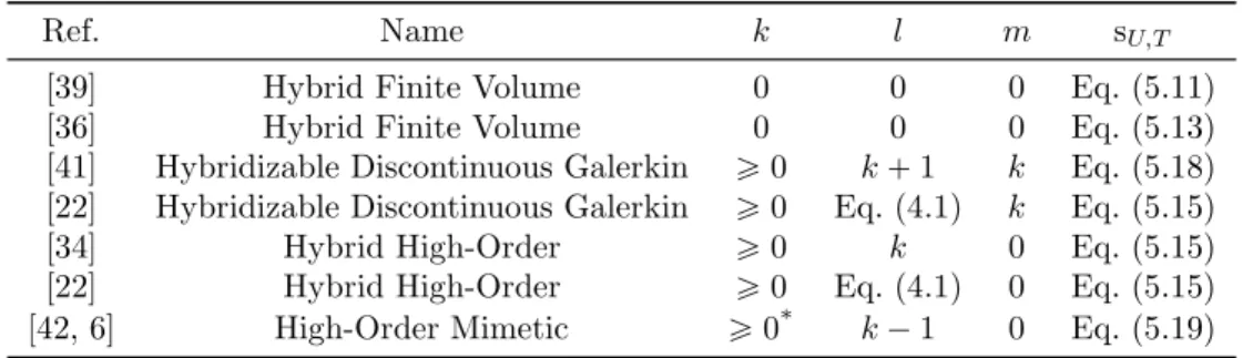
Ref. Name k l m sU,T
[39] Hybrid Finite Volume 0 0 0 Eq. (5.11) [36] Hybrid Finite Volume 0 0 0 Eq. (5.13) [41] Hybridizable Discontinuous Galerkin ě 0 k` 1 k Eq. (5.18) [22] Hybridizable Discontinuous Galerkin ě 0 Eq. (4.1) k Eq. (5.15) [34] Hybrid High-Order ě 0 k 0 Eq. (5.15) [22] Hybrid High-Order ě 0 Eq. (4.1) 0 Eq. (5.15) [42, 6] High-Order Mimetic ě 0* k´ 1 0 Eq. (5.19)
Table 2: Examples of methods originally introduced in primal formulation. * The High-Order
Mimetic method enters the present framework only for kě 1.
5.5
Examples
We collect in this section a few examples of discontinuous skeletal methods originally introduced in a primal formulation which can be traced back to (5.9). Each method is uniquely defined by prescribing the three polynomial degrees k, l, and m (in accordance with (4.1)) and the expression of the local stabilization bilinear form sU,T for a generic mesh element T P Th. A synopsis is
provided in Table 2.
Example 11 (The Hybrid Finite Volume method of [39] and its generalization of [36]). The Hybrid Finite Volume method of [39, Section 2.1] corresponds to k“ l “ m “ 0. In this case, an explicit expression for the gradient operator G0T defined by (5.4) is available: For all vT P U
0,0 T , G0TvT “ 1 |T |d ÿ FPFT |F |d´1vFnT F. (5.10)
For every element T P Th, the stabilization bilinear form is such that
sU,TpuT, vTq “ ÿ FPFT |F |d´1 η hT F δ0T FuTδ 0 T FvT, (5.11)
where ηą 0 is a user-dependent stabilization parameter, hT F as in Example 5 and the face-based
residual operator δ0 T F : U
0,0
T Ñ P0pF q is such that, denoting by xF the barycenter of F and by
xT an arbitrary point associated with T which may or may not belong to T ,
δ0T FvT :“ vT ` G0TvT¨pxF´ xTq ´ vF. (5.12)
In [36, Section 2.2], the following generalization of (5.11) is proposed: For a given positive definite matrix BT “ pBT F F1qF,F1PF T, sU,TpuT, vTq “ ÿ FPFT ÿ F1PF T δ0T FuTB T F F1δT F0 1vT. (5.13)
Example 12 (The Hybrid High-Order method of [34] and the variants of [22]). The original Hybrid High-Order method of [34] corresponds to the choice l“ k and m “ 0. In [22], variants corresponding to l“ k ´ 1 (when k ě 1) and l “ k ` 1 have also been proposed. Let an element T P Th be fixed, and define the potential reconstruction operator pkT`1 : Uk,lT Ñ Pk`1pT q such
that, for all vT P U k,l T , ∇pkT`1vT “ G k TvT and pp k`1 T vT ´ vT,1qT “ 0. (5.14)
Note that the first condition makes sense since, having supposed m “ 0, GkTvT P G l T. The
stabilization bilinear form is defined as follows: sU,TpuT, vTq “ ÿ FPFT h´1F pδ k T FuT, δT Fk vTqF, (5.15)
where, for all F P FT, the face-based residual operator δkT F : U k,l T Ñ P
kpF q is such that, for all
vT P U k,l T , δT Fk vT “ πFk ` pkT`1vT ´ vF´ πlTpp k`1 T vT´ vTq ˘ . (5.16)
As already observed in [34, Section 2.5], in the lowest-order case k “ 0 the face-based residuals defined by (5.12) and (5.16) coincide, and the stabilization (5.15) can be recovered from (5.13) selecting BT “ diagph´1F |F |d´1qFPFT (the only difference with respect to (5.11) is the change of
local scaling hT F Ð hF).
Example 13(The Crouzeix–Raviart finite element). Let T be an element belonging to a matching simplicial mesh Thwith barycenter xT, and consider the Crouzeix–Raviart element NCpT q of [25].
We study the solution of problem (5.9) using the Hybrid Finite Volume method of Example 11 (or, equivalently, the Hybrid High-Order method of Example 12 with k “ l “ m “ 0) but with right-hand side discretized as ÿ
TPTh
pf, p1TvTqT, (5.17)
where the potential reconstruction p1
T is defined according to (5.14) but with average value on T
set to 1 d`1
ř
FPFT vF (here, hT F is the orthogonal distance of xT from F ). We start by noticing
that it holds π0
Fp1TvT “ p1TvTpxFq “ vF for all vT P U k,l
T and all F P FT with xF barycenter of
F. As a consequence, for the face-based residual operator (5.12) it holds for all vT P U 0,0 T that
δ0T FvT “ ´π0Tpp1TvT ´ vTq “ vT´ p1TvTpxTq.
Then, observing that element-based DOFs do not contribute to the consistency term in (5.6) nor to the right-hand side, we infer that the stabilization term is actually enforcing the condition p1
TvTpxTq “ vT for all T P Th. As a result, denoting by uh P U 0,0
h,0 the solution of problem (5.9)
with right-hand side modified as in (5.17), the piecewise affine field equal to p1
TuT inside each
mesh element T P Thcoincides with the Crouzeix–Raviart solution (3.4).
Example 14(The Hybridizable Discontinuous Galerkin method of [41] and the variants of [22]). The Hybridizable Discontinuous Galerkin originally proposed in [41, Remark 1.2.4] corresponds to the case l“ k ` 1 and m “ k and stabilization
sU,TpuT, vTq “
ÿ
FPFT
h´1F pπk
FpuT ´ uFq, πFkpvT ´ vFqqF. (5.18)
As pointed out in [22, Remark 2], this stabilization coincides with (5.15) when l“ k ` 1. Moti-vated by this remark, variants corresponding to the choices l“ k ´ 1 (when k ě 1) and l “ k and m“ k are proposed therein. It is worth noting here that the original Hybridizable Discontinuous Galerkin method of [20, 23] does not fit in the present framework since the corresponding stabi-lization bilinear form is only polynomially consistent up to degree k, i.e., it does not satisfy (S21).
Correspondingly, the orders of convergence are reduced (cf. [22, Table 1] for further details). Example 15 (The High-Order Mimetic method of [42, 6]). The High-Order Mimetic method of [42] (subsequently referred to as Nonconforming Virtual Element method in [6]) provides a high-order generalization of the concepts underlying Mimetic Difference Methods (cf., e.g., [13]). Its lowest-order version, corresponding to the case k“ 0 and l “ ´1, violates (4.1), and therefore does not enter our unified framework. For kě 1, on the other hand, it corresponds to the choices l“ k ´ 1 and m “ 0. To write the corresponding bilinear form, define the finite-dimensional local virtual space
UkpT q :“ vT P H1pT q | △vT P Pk´1pT q and p∇vTq|F¨nT F P PkpF q for all F P FT
( . Clearly, Pk`1pT q Ă UkpT q, and it can be proved that Ik,k´1
U,T defines an isomorphism from U kpT q
to UTk,k´1. Denote by ShomT : U
canonical basis of UkpT q is spectrally equivalent to the unit matrix. The stabilization bilinear
form is obtained setting, for all uT, vT P U k,l T ,
sU,TpuT, vTq :“ hd´2T S hom
T ppk`1T uT´ uT,pk`1T vT´ vTq, (5.19)
where uT and vT are the unique functions in UkpT q such that uT “ I k,k´1
U,T uT and vT “ I k,k´1 U,T vT,
while the operator pkT`1is defined by (5.14). The stabilization (5.19) essentially corresponds to
pe-nalizing in a least-square sense the high-order differences πl
Tppk`1T vT ´ vTq and πFkppk`1T vT´ vFq,
F P FT, with scaling factor choosen so that the uniform equivalence in (S11) holds.
6
From mixed to primal methods
In this section we obtain from (4.18) an equivalent primal problem by hybridization. The pri-mal hybrid problem is then shown to belong to the family (5.9) of pripri-mal discontinuous skeletal methods.
6.1
Mixed hybrid formulation of mixed methods
We define the bilinear form bh: qΣ k,l,m h ˆ U k,l h Ñ R (with spaces qΣ k,l,m h and U k,l h defined by (4.14)
and (5.7), respectively) such that, for allpτh, vhq P qΣ k,l,m h ˆ U k,l h , bhpτh, vhq :“ ÿ TPTh bTpτT, vTq, bTpτT, vTq :“ pD l TτT, vTqT ´ ÿ FPFT pτT F, vFqF. (6.1)
For further use, we note that it holds for all T P Th, all τT P Σ k,l,m T , and all vT P U k,l T , bTpτT, vTq “ ´pτG,T, ∇vTqT ` ÿ FPFT pτT F, vT ´ vFqF, (6.2)
as can be easily checked replacing Dl
T by its definition (4.6) and accounting for Remark 1. Hence,
using the Cauchy–Schwarz inequality and recalling the definitions (4.4) and (5.2) of }¨}Σ,T and
}¨}U,T, we infer the following boundedness result for bT:
|bTpτT, vTq| ď }τT}Σ,T}vT}U,T. (6.3)
Problem 3 (Mixed hybrid problem). Find pσh, uhq P qΣ k,l,m h ˆ U k,l h,0 such that, @T P Th, mTpσT, τTq ` bTpτT, uTq “ 0 @τT P Σ k,l,m T , (6.4a) ´bhpσh, vhq “ pf, vhq @vhP U k,l h,0. (6.4b)
Compared to the mixed problem (4.18), the single-valuedness of interface flux unknowns is enforced here by Lagrange multipliers (corresponding to the skeletal DOFs in Uk,lh,0) instead of being embedded in the discrete space. Equation (6.4a) defines a set of local constitutive relations connecting flux to potential DOFs inside each mesh element. Equation (6.4b), on the other hand, expresses local balances and a global transmission condition. In what follows, we will eliminate flux unknowns by locally inverting (6.4a), ending up with a problem in the hybrid potential unknowns only.
6.2
Mixed-to-primal potential-to-flux operator
For all T P Th, we define the local mixed-to-primal potential-to-flux operator ςk,l,mT : U k,l T Ñ Σ
k,l,m T
such that, for all vT P U k,l T ,
mTpςk,l,mT vT, τTq “ ´bTpτT, vTq @τT P Σ k,l,m
Recalling the reformulation (6.2) of bT, (6.5) equivalently rewrites mTpςk,l,mT vT, τTq “ p∇vT, τG,TqT ` ÿ FPFT pvF ´ vT, τT FqF @τT P Σ k,l,m T . (6.6)
We next state some useful properties for the potential-to-flux operator.
Lemma 16 (Properties of the mixed-to-primal potential-to-flux operator). Let a mesh element T P Th be given and let sΣ,T be a bilinear form satisfying Assumption 1. Then, the corresponding
potential-to-flux operator ςk,l,mT given by (6.5) is well defined and has the following properties:
1) Stability and continuity. For all vT P U k,l
T , it holds
}ςk,l,mT vT}Σ,T « }vT}U,T, (6.7)
with norms }¨}Σ,T and}¨}U,T defined by (4.4) and (5.2), respectively.
2) Commuting property. For all wP Pk`1pT q, we have
ςk,l,mT I k,l U,Tw“ I
k,l,m
Σ,T ∇w. (6.8)
3) Link with the discrete gradient operator. It holds, with operators GkT and S k
T defined by (5.4)
and (4.8), respectively, that
GkT :“ Sk T ˝ ς
k,l,m
T . (6.9)
Proof. Problem (6.5) is well-posed owing to assumption (S1) expressing the coercivity of mT. As
a result, ςk,l,mT is well defined.
1) Stability and continuity. Using (S1) followed by the definition (6.5) of ςk,l,mT and the
bound-edness (6.3) of bT, we infer, for all vT P U k,l T , }ςk,l,mT vT}2Σ,T À }ς k,l,m T vT}2m,T “ ´bTpς k,l,m T vT, vTq ď }ς k,l,m T vT}Σ,T}vT}U,T. (6.10)
To prove the converse inequality, let τT P Σ k,l,m
T in (6.6) be such that τT “ ∇vT and τT F “
h´1F pvF ´ vTq for all F P FT, and observe that
}vT}2U,T “ mTpςk,l,mT vT, τTq À }ς k,l,m
T vT}Σ,T}τT}Σ,T “ }ςTk,l,mvT}Σ,T}vT}U,T, (6.11)
where we have used the Cauchy–Schwarz inequality together with (S1) to bound mT and the
definitions (4.4) of}¨}Σ,T and (5.8) of}¨}U,T to infer}τT}Σ,T “ }vT}U,T and conclude.
2) Commuting property. Let w P Pk`1pT q. Using the definition (6.5) of ςk,l,m
T with vT “ I k,l U,Tw
and recalling (6.1), we infer, for all τT P Σ k,l,m T , mTpςk,l,mT I k,l U,Tw, τTq “ ´pπ l Tw,DlTτTqT` ÿ FPFT pπk Fw, τT FqF “ ´pw, Dl TτTqT` ÿ FPFT pw, τT FqF “ p∇w, PkTτTqT, (6.12)
where we have used the definitions (2.1) of πl
T and πFk to pass to the second line and the
defini-tion (4.7) of PkT to conclude. On the other hand, using the definition (4.13a) of mT followed by
the polynomial consistency (4.12) of SkT together with (S2), for all τT P Σ k,l,m T we have that mTpIk,l,mΣ,T ∇w, τTq “ pS k TI k,l,m Σ,T ∇w, S k TτTqT ` sΣ,TpIk,l,mΣ,T ∇w, τTq “ p∇w, SkTτTqT “ p∇w, PkTτTqT, (6.13)
where the last equality follows from the definition (4.8) of SkT together with the orthogonal
de-composition (2.2). Subtracting (6.13) from (6.12), we infer, for all τT P Σ k,l,m T , mTpςk,l,mT I k,l U,Tw´ I k,l,m Σ,T ∇w, τTq “ 0,
3) Link with the discrete gradient operator. Let vT P U k,l T , τ P S k,m T , and set τT :“ I k,l,m Σ,T τ.
Recalling the definition (4.13a) of mT, and using the polynomial consistency (4.12) of SkT together
with (S2), it is readily inferred that
mTpςk,l,mT vT, τTq “ ppS k T ˝ ς
k,l,m
T qvT, τqT. (6.14)
On the other hand, recalling the definitions (4.3) of Ik,l,mΣ,T and (6.1) of bT, we get
bTpτT, vTq “ pvT,DlTτTqT´ ÿ FPFT pvF, τT FqF “ pvT, πTlpdiv τ qqT ´ ÿ FPFT pvF, πFkpτ ¨nT FqqF “ pvT,div τqT ´ ÿ FPFT pvF, τ¨nT FqF “ ´pGkTvh, τqT, (6.15)
where we have used the commuting property (4.9) of Dl
T in the second line and the definition (2.1)
of πl
T and πFk and (5.4) of G k
T in the third. To conclude, plug (6.14) and (6.15) into the
defini-tion (6.5) of ςk,l,mT .
6.3
Equivalent primal formulations of mixed methods
We start by showing a link among problems (4.18), (6.4), and the following Problem 4 (Primal hybrid problem). Findpσh, uhq P qΣ
k,l,m h ˆ U k,l h,0 such that σT “ ς k,l,m T uT @T P Th, (6.16a)
with potential-to-flux operator ςk,l,mT defined by (6.5) and uh solution of
ahpuh, vhq “ pf, vhq @vhP U k,l
h,0, (6.16b)
where the bilinear form ah on Uk,lh ˆ U k,l h is such that ahpuh, vhq :“ ÿ TPTh aTpuT, vTq, aTpuT, vTq :“ mTpς k,l,m T uT, ς k,l,m T vTq. (6.17)
The well-posedness of (6.16b) is an immediate consequence of point 1) in Theorem 18 below. Theorem 17(Link among the mixed, mixed hybrid and primal hybrid problems). For all T P Th,
let sΣ,T satisfy Assumption 1. Letpσh, uhq P qΣ k,l,m h ˆU
k,l
h,0, and let uhP Uhl be such that uh|T “ uT
for all T P Th. Then, the following statements are equivalent:
(i) pσh, uhq solves the mixed hybrid problem (6.4);
(ii) σhP Σ k,l,m
h andpσh, uhq solves the mixed problem (4.18);
(iii) pσh, uhq solves the primal hybrid problem (6.16).
Proof. The equivalence (i) ðñ (ii) classically follows from the theory of Lagrange multipliers. Let us prove the equivalence (i) ðñ (iii). We first show that if pσh, uhq solves the mixed hybrid
problem (6.4), then it solves the primal hybrid problem (6.16). Equation (6.16a) immediately follows from (6.4a) recalling the definition (6.5) of the potential-to-flux operator. As a consequence, it holds for all T P Th and all vT P U
k,l T ,
´bTpσT, vTq “ ´bTpςk,l,mT uT, vTq “ mTpςk,l,mT uT, ς k,l,m
where we have used the definition (6.5) of the potential-to-flux operator together with the sym-metry of mT in the second equality and the definition (6.17) of the bilinear form aT to conclude.
This implies that (6.4b) is equivalent to (6.16b). By similar arguments, we can prove that if pσh, uhq solves the primal hybrid problem (6.16), then it solves the mixed hybrid problem (6.4),
thus concluding the proof.
We close this section with our main result, viz. the existence of a primal method belonging to the family (5.9) whose solution coincides with that of the mixed method (4.18) for given stabilization bilinear forms satisfying Assumption 1. In the light of Theorem 17, it suffices to state the equivalence with respect to the corresponding mixed hybrid formulation (6.4).
Theorem 18 (Link with the family of primal discontinuous skeletal methods). For all T P Th,
let sΣ,T satisfy Assumption 1 and set with ςk,l,mT defined by (6.5):
sU,TpuT, vTq :“ sΣ,Tpςk,l,mT uT, ς k,l,m
T vTq. (6.18)
Then,
1) Properties of sU,T. The stabilization bilinear forms sU,T, T P Th, satisfy Assumption 2;
2) Link with primal methods. uh P U k,l
h,0 solves the primal problem (5.9) with stabilization as
in (6.18) if and only ifpσh, uhq P qΣ k,l,m h ˆ U
k,l
h,0with σhsuch that σT “ ς k,l,m
T uT for all T P Th
solves the mixed hybrid problem (6.4).
Proof. 1) Properties of sU,T. Let T P Th. The bilinear form sU,T is clearly symmetric and
positive semi-definite. It then suffices to prove conditions (S11) and (S21). To prove (S11), observe
that for all vT P U k,l
T we have
}vT}a,T “ }ςk,l,mT vT}m,T« }ςk,l,mT vT}Σ,T « }vT}U,T,
where we have used the definition (6.17) of aT, (S1), and the stability and continuity (6.7) of
ςk,l,mT . Let us prove (S21). Letting wP P
k`1pT q, for all v T P U k,l T we have sU,TpI k,l U,Tw, vTq “ sΣ,Tpς k,l,m T I k,l U,Tw, ς k,l,m T vTq “ sΣ,TpI k,l,m Σ,T ∇w, ς k,l,m T vTq “ 0,
where we have used the definition (6.18) of sU,T, the commuting property (6.8), and (S2).
2) Link with primal methods. Compare the primal hybrid formulation (6.16) with the primal formulation (5.9) and recall the equivalence with the mixed hybrid formulation (6.4) stated in Theorem 17.
7
From primal to mixed methods
In this section we show that the primal discontinuous skeletal methods of Section 5 with m“ 0 can be recast into the mixed formulation introduced in Section 4. This enables us to close the circle and show a precise equivalence relation between the family (4.18) of mixed discontinuous skeletal methods and the family (5.9) of primal discontinuous skeletal methods.
7.1
Primal-to-mixed potential-to-flux operator
We assume from this point on that, for a given integer kě 0, l is as in (4.1) and m“ 0.
The crucial ingredient is the primal-to-mixed potential-to-flux operator ςk,lT : U k,l T Ñ Σ
k,l,0 T such
that, for all wT P U k,l T , ς k,l T wT solves ´ bTpςk,lT wT, vTq “ aTpwT, vTq @vT P U k,l T . (7.1)
The use of a similar notation as for the mixed-to-primal potential-to-flux operator is motivated by the fact that these two operators share the same properties (compare Lemmas 16 and 19) and play very much the same role.
Lemma 19 (Properties of the primal-to-mixed potential-to-flux operator). Let a mesh element T P Th be given and let sU,T be a bilinear form satisfying Assumption 2. Then, the corresponding
potential-to-flux operator ςk,lT given by (6.5) is well defined and has the following properties:
1) Stability and continuity. For all vT P U k,l
T , it holds with norms }¨}Σ,T and }¨}U,T defined
by (4.4) and (5.2), respectively,
}ςk,lT vT}Σ,T « }vT}U,T. (7.2)
2) Commuting property. For all wP Pk`1pT q, we have
ςk,lT Ik,lU,Tw“ Ik,l,0Σ,T∇w. (7.3)
3) Link with the discrete gradient operator. It holds, with operators GkT, P k
T, and S k
T defined
by (5.4), (4.7), and (4.8), respectively, that
GkT “ PkT ˝ ς k,l T “ S k T ˝ ς k,l T . (7.4)
Additionally, ςk,lT defines an isomorphism from U k,l
T,˚ (cf. (5.3)) to Σ k,l,0 T .
Proof. Let T P Th. To show that ςk,lT is well defined we prove the following inf-sup condition: For
all τT P Σ k,l,0 T , }τT}Σ,T ď S :“ sup vTPUk,lT ,˚zt0U,Tu bTpτT, vTq }vT}U,T . (7.5) Let vτ,T P U k,l
T be such that ∇vτ,T “ τT and vτ,F ´ vτ,T “ hFτT F (vτ,T is defined up to an
element of Ik,lU,TP0pT q, coeherently with the fact that we write U k,l
T,˚ in the supremum). It can be
checked that }vτ,T}U,T “ }τT}Σ,T and it holds, recalling the reformulation (6.2) of the bilinear
form bT,
}τT}2Σ,T “ ´bTpτT, vτ,Tq ď S}vτ,T}U,T “ S}τT}Σ,T,
which proves (7.5). To prove the well-posedness of problem (7.1) it only remains to observe that, for all vT P I
k,l
U,TP0pT q, equation (7.1) becomes the trivial identity 0 “ 0, which can be intepreted
as a compatibility condition. Finally, the fact that ςk,lT defines an isomorphism from Uk,lT,˚to Σk,l,0T follows observing that ςk,lT is injective as a result of (7.5) and dimpU
k,l
T,˚q “ dimpΣ k,l,0 T q.
1) Stability and continuity. Combining the inf-sup condition (7.5) with the definition (7.1) of ςk,lT , and using the Cauchy–Schwarz inequality followed by (S1), we get for all vT P U
k,l T that }ςk,lT vT}Σ,T ď sup wTPUk,lT ,˚zt0U,Tu bTpς k,l T vT, wTq }wT}U,T “ sup wTPUk,lT ,˚zt0U,Tu aTpvT, wTq }wT}U,T À }vT}U,T.
On the other hand, (S1) followed by the definition (7.1) of ςk,lT and the boundedness (6.3) of the
bilinear form bT yields
}vT}2U,T À aTpvT, vTq “ ´bTpς k,l
T vT, vTq ď }ς k,l
T vT}Σ,T}vT}U,T,
2) Commuting property. Let wP Pk`1pT q. For all v T P U k,l T it holds ´bTpςk,lT Ik,lU,Tw, vTq “ aTpIk,lU,Tw, vTq “ p∇w, G k TvTqT “ ´bTpIk,l,0Σ,T∇w, vTq,
where we have used the definition (7.1) of ςk,lT in the first equality, the definition (5.6) of aTtogether
with (S21) in the second equality, and concluded recalling the definitions (5.4) of Gk
T, (4.3) of I k,l,0 Σ,T, and (6.1) of bT. As a consequence, bTpIk,l,0Σ,T∇w´ ς k,l T I k,l U,Tw, vTq “ 0 @vT P U k,l T ,
which, accounting for the inf-sup condition (7.5), implies (7.4). 3) Link with the discrete gradient operator. Let vT P U
k,l
T and w P Pk`1pT q. Recalling the
definitions (6.1) of bT and (5.1) of I k,l
U,T, we infer that
´bTpςk,lT vT, I k,l U,Twq “ ´pD l Tς k,l T vT, π l TwqT ` ÿ FPFT ppςk,lT vTqT F, πkFwqF “ ´pDl Tς k,l T vT, wqT ` ÿ FPFT ppςk,lT vTqT F, wqF “ ppPkT ˝ ς k,l T qvT, ∇wqT,
where we have used the definition (2.1) of πl T and π
k
F to pass to the second line and the
defini-tion (4.7) of PkT to conclude. On the other hand, by the definition (5.6) of aT together with the
polynomial consistency of GkT (a consequence of (5.5)) and (S21), we have
aTpvT, I k,l
U,Twq “ pG k
TvT, ∇wqT.
Substituting the above relations into the definition (7.1) of ςk,lT we infer that G k TvT “ P k T ˝ ς k,l T .
Additionally, since we have supposed m“ 0, we also have SkT “ P k
T, thus concluding the proof.
7.2
Equivalent mixed formulation of primal methods
We close this section by showing the existence of a mixed method belonging to the family (4.18) whose solution coincides with that of the primal problem (5.9). In the light of Theorem 17, we state the equivalence result in terms of the corresponding mixed hybrid formulation (6.4). Theorem 20(Link with the family of mixed discontinuous skeletal methods). For all T P Th, let
sU,T satisfy Assumption 2 and set, for all σT, τT P Σ k,l,0 T ,
sΣ,TpσT, τTq :“ sU,Tppςk,lT q´1σT,pς k,l
T q´1τTq, (7.6)
where it is understood thatpςk,lT q´1τT andpς k,l
T q´1σT are defined up to an element of I k,l U,TP0pT q.
Then,
1) Properties of sΣ,T. The stabilization bilinear forms sΣ,T, T P Th satisfy Assumption 1;
2) Link with mixed methods. pσh, uhq P qΣ k,l,0 h ˆ U
k,l
h,0 solves the mixed hybrid problem (6.4) with
stabilization as in (7.6) if and only if uh solves the primal problem (5.9) and, for all T P Th,
σT “ ς k,l
T uT with ς k,l
T defined by (7.1).
Proof. 1) Properties of sΣ,T. Let T P Th. The bilinear form sΣ,T is clearly symmetric and
positive semi-definite. It then suffices to prove conditions (S1) and (S2). Let us start by (S1). Recalling the definition (4.13a) of the bilinear form mT, property (7.4) for the potential-to-flux
operator ςk,lT defined by (7.1), and (7.6), we infer for all wT, vT P U k,l T that
mTpςk,lT wT, ς k,l
Let now τT P Σ k,l,0 T be such that τT “ ς k,l T vT with vT P U k,l
T (the existence of such vT, defined
up to an element of Ik,lU,TP0pT q, follows from Lemma 19). We have that
}τT}Σ,T « }vT}U,T « }vT}a,T “ }τT}m,T,
where the first norm equivalence follows from (7.2), the second from (S21), and the last one
from (7.7). Property (S1) follows.
Let us now prove (S2). Let χP GkT be such that χ“ ∇w with w P Pk`1pT q. For all vT P U k,l T it holds, sΣ,TpIk,l,0Σ,Tχ, ς k,l T vTq “ sU,Tppς k,l T q´1I k,l,0 Σ,Tχ, vTq “ sU,TpI k,l U,Tw, vTq “ 0,
where we have used the definition (7.6) of sΣ,T, the commuting property (7.3), and concluded
using (S21).
2) Link with mixed methods. We let pσh, uhq P qΣ k,l,0 h ˆ U
k,l
h,0 solve the mixed hybrid
prob-lem (6.4) with sΣ,T given by (7.6), and we show that uh solves (5.9) and σT “ ς k,l T uT for all T P Th. Making τT “ ς k,l T vT with vT P U k,l T in (6.4a), it is inferred 0“ mTpσT, ς k,l T vTq ` bTpςk,lT vT, uTq “ mTpσT ´ ς k,l T uT, ς k,l T vTq. Since Σk,l,0T “ ς k,l T U k,l
T as a result of Lemma 19 and vT is arbitrary in U k,l
T , this means that
σT “ ς k,l
T uT @T P Th. (7.8)
Plugging this relation into (6.4b), and recalling the definition (7.1) of ςk,lT , we infer that it holds
for all vhP U k,l h,0, pf, vhq “ ´ ÿ TPTh bTpσT, vTq “ ´ ÿ TPTh bTpςk,lT uT, vTq “ ahpuh, vhq,
which shows that uh solves the primal problem (5.9). Following a similar reasoning one can prove
that, if uhsolves (5.9), then pσh, uhq with σT “ ς k,l
T uT for all T P Th solves (6.4).
8
Analysis
In this section we carry out a unified convergence analysis encompassing both mixed and primal discontinuous skeletal methods. Recalling Theorems 17, 18, and 20, we focus on the mixed hybrid problem (6.4). Let three integers kě 0 and l, m as in (4.1) be fixed, set Xk,l,mh :“ qΣ
k,l,m h ˆ U
k,l h,0,
and define the bilinear form Ah: Xk,l,mh ˆ X k,l,m
h Ñ R such that
Ahppσh, uhq, pτh, vhqq :“ mhpσh, τhq ` bhpτh, uhq ´ bhpσh, vhq. (8.1)
Problem (6.4) admits the following equivalent reformulation: Findpσh, uhq P qΣ k,l,m h ˆ U k,l h,0 such that, Ahppσh, uhq, pτh, vhqq “ pf, vhq @pτh, vhq P qΣk,l,mh ˆ U k,l h,0. (8.2)
8.1
Stability and well-posedness
We equip the space Xk,l,mh with the norm}¨}X,hsuch that, for allpτh, vhq P X k,l,m h , }pτh, vhq} 2 X,h:“ }τh} 2 Σ,h` }vh} 2 U,h, with norms}¨}Σ,h on qΣ k,l,m
Lemma 21 (Well-posedness). For all pχh, whq P X k,l,m h it holds }pχh, whq}X,hÀ sup pτh,vhqPX k,l,m h zt0X,hu Ahppχh, whq, pτh, vhqq }pτh, vhq}X,h . (8.3)
Consequently, problem (8.2) is well-posed.
Proof. We start by proving the following inf-sup condition for bh: For all vhP U k,l h,0, }vh}U,hÀ sup τ hP qΣ k,l,m h zt0Σ,hu bhpτh, vhq }τh}Σ,h . (8.4) Fix an element vh P U k,l h,0, and let τv,h P qΣ k,l,m
h be such that, for all T P Th, τv,T “ ∇vT and
τv,T F “ h´1F pvF ´ vTq. Denoting by S the supremum in (8.4) from (6.2) it is inferred that
}vh}2U,h“ bhpτv,h, vhq ď S}τv,h}Σ,h,
and (8.4) readily follows observing that, by the definitions (4.4) and (5.2) of the local norms, }τv,T}Σ,T “ }vT}U,T. The inf-sup condition (8.3) on Ah and the well-posedness of problem (6.4)
are then classical consequences of the }¨}Σ,h-coercivity of mh (itself a consequence of (S1)) and
the inf-sup condition (8.4) on bh; cf., e.g., [14].
8.2
Energy error estimate
We estimate the error defined as the difference between the solution of the mixed hybrid prob-lem (6.4) and the projectionpσph,puhq P qΣ
k,l,m h ˆ U
k,l
h,0 of the exact solution defined as follows:
p σh:“ I k,l,m Σ,h ∇hquh @T P Th, puh:“ I k,l U,hu,
where quh P Pk`1pThq is such that, for all T P Th, quT :“ quh|T is the local elliptic projection of u
satisfying
∇uqT “ πkG,T∇u and pquT ´ u, 1qT “ 0, (8.5)
while Ik,l,mΣ,h is the global flux reduction map on qΣ k,l,m
h whose restriction to every mesh elements T P
Th coincides with Ik,l,mΣ,T defined by (4.3). Optimal approximation properties for quhon admissible
mesh sequence are proved in [34, Lemma 3] and, in a more general framework, in [29]. Theorem 22 (Energy error estimate). Let uP H1
0pΩq be the weak solution of problem (1.1), and
assume the additional regularity uP Hk`2pΩq. Then, it holds
}pσh´σph, uh´ puhq}X,hÀ hk`1}u}Hk`2pΩq. (8.6)
Proof. The following error equation descends from (8.2): For allpτh, vhq P qΣ k,l,m h ˆ U
k,l h,0,
Ahppσh´σph, uh´ puhq, pτh, vhqq “ Ehpτh, vhq,
with consistency error
Ehpτh, vhq :“ pf, vhq ` bhpσph, vhq ´ mhpσph, τhq ´ bhpτh,puhq. (8.7)
Recalling the inf-sup condition (8.3), we then have that
}pσh´σph, uh´ puhq}X,hÀ sup pτh,vhqPX k,l,m h zt0X,hu Ehpτh, vhq }pτh, vhq}X,h . (8.8)