Custom and interactive environments in StarLogo Nova for computational modeling

(1)

Custom and Interactive Environments in StarLogo Nova

for Computational Modeling

by Malcolm X. Wetzstein

B.S., Computer Science and Engineering,

Massachusetts Institute of Technology (2019)

Submitted to the

Department of Electrical Engineering and Computer Science

in Partial Fulfillment of the Requirements for the Degree of

Master of Engineering in Electrical Engineering and Computer Science

at the

Massachusetts Institute of Technology

August 2019

© Massachusetts Institute of Technology 2019. All rights reserved.

Author: ____________________________________________________________________ Department of Electrical Engineering and Computer Science

August 23rd_{, 2019}

Certified by: ____________________________________________________________________ Eric Klopfer, Professor, Thesis Supervisor

August 23rd_{, 2019}

Accepted by: ____________________________________________________________________ Katrina LaCurts, Chair, Master of Engineering Thesis Committee

(2)

(3)

3

Custom and Interactive Environments in StarLogo Nova

for Computational Modeling

by Malcolm X. Wetzstein

August 23

rd

_{, 2019}

In partial Fulfillment of the Requirements for the

Degree of Master of Engineering in

Electrical Engineering and Computer Science

Abstract

StarLogo Nova is an agent-based simulation and game programming application geared towards

classroom learning. In many cases, StarLogo Nova can be an effective computational modeling tool, allowing students to apply their knowledge and gain a greater understanding of scientific concepts. However, there are many computational models that are difficult to implement in StarLogo Nova or cannot be implemented. This can be partly attributed to the fact that agents are the only programmable and customizable entity in StarLogo Nova and are limited to interactions with other agents. We expand the set of computational models possible within StarLogo Nova by adding new features and capabilities; namely an editable and programmable 3D environment for agents to interact with. We add the

capability for users to program real-time interactions between agents and their environment. A dynamic and custom environment opens up the possibility for new computational models and simplifies the implementation of others.

Thesis Supervisor: Eric Klopfer

Title: Professor

(4)

(5)

5

List of Figures

Figure 1: Top: StarLogo Nova viewport and workspace. ... 10

Figure 2: A program in StarLogo Nova described graphically using blocks. ... 12

Figure 3: Editable terrain from StarLogo Nova’s predecessor, StarLogo TNG. ... 16

Figure 4: Previous terrain in StarLogo Nova. ... 17

Figure 5: An example of a triangle mesh. ... 18

Figure 6: Location of points in a floor patch. ……….. 21

Figure 7: Wall patches. ……… 22

Figure 8: Selection in the Terrain Editor. ……… 24

Figure 9: The raise command. ……… 25

Figure 10: The mound command. ……… 26

Figure 11: The level command. ………. 29

Figure 12: The close seams command. ……… 30

Figure 13: The ramp command. ……… 31

Figure 14: Diagram of ramp algorithm for computing linear transitions. ……… 32

Figure 15: Agent terrain traversal and altitude. ……… 38

Figure 16: Definition of terrain height. ……… 39

Figure 17: The yank grid command. ……….. 41

Figure 18: Template for yank grid weights. ………. 42

Figure 19: Correspondence between floor patch points and underlying triangle vertices. ……… 55

(8)

8

1 Introduction

StarLogo Nova is an agent-based simulation and game programming application geared towards

classroom learning. In many cases, StarLogo Nova can be an effective computational modeling tool, allowing students to apply their knowledge and gain a greater understanding of scientific concepts. However, there are many computational models that are difficult to implement in StarLogo Nova or cannot be implemented. This can be partly attributed to the fact that agents are the only programmable and customizable entity in StarLogo Nova and are limited to interactions with other agents. We expand the set of computational models possible within StarLogo Nova by adding new features and capabilities; namely an editable and programmable 3D environment for agents to interact with. We add the

capability for users to program real-time interactions between agents and their environment. A dynamic and custom environment opens up the possibility for new computational models and simplifies the implementation of others.

Section 1 provides more background information on what the StarLogo Nova application is, the intended purposes of the application, and how it is used. Section 2 elaborates on StarLogo Nova’s previous representation of the environment and the role that it plays in a simulation. More importantly, Section 2 explains how the work of this thesis changes the representation of the environment so that new features can be added. Sections 3 and 4 explain the new features added by the work of this thesis, with Section 3 focusing on the new features for editing the environment and Section 4 focusing on the new features that allow programmable interactions between agents and the environment. Section 5 sheds light on how the software that implements the new features is organized and explains the interface that it exposes to the rest of StarLogo Nova that make the new features possible. Section 5 also explains some key implementation details. Section 6 provides an example of a concrete use case for the new features we propose. Section 7 summarizes how the new features fulfill the purpose of this

(9)

9

thesis. Section 8 provides several starting points for future work to either extend or improve the work of this thesis.

1.1 Purpose of StarLogo Nova

StarLogo Nova is a flexible tool that can be used to create many kinds of simulations, including

games. However, StarLogo Nova is primarily a tool for creating computational models. A computational model is a computer simulation used to study the behavior of a system. The design of StarLogo Nova is particularly geared towards creating models of complex systems, systems with many components that interact with one another to produce complex behavior [Melnik 2015]. An example of a complex system is the relationship between populations of a predator species and their prey. The relationship between the two populations can be modeled in a computer simulation. The computer simulation can then be studied to better understand how the size of one population affects the other.

The target audiences of StarLogo Nova are secondary school students and educators. As stated previously, StarLogo Nova is a powerful tool for teaching scientific concepts to students. By having students create computational models of a scientific phenomenon, they gain greater understanding of that phenomenon and dispel misconceptions. Working in StarLogo Nova also allows students to start developing computational thinking skills, the ability to express problems in a way that computers can solve, earlier in their education [Lee et al. 2014].

1.2 What is StarLogo Nova?

In this section we explain the nature of the StarLogo Nova application; what platform the application is on, the user interface of the application, and how a user uses the application. StarLogo

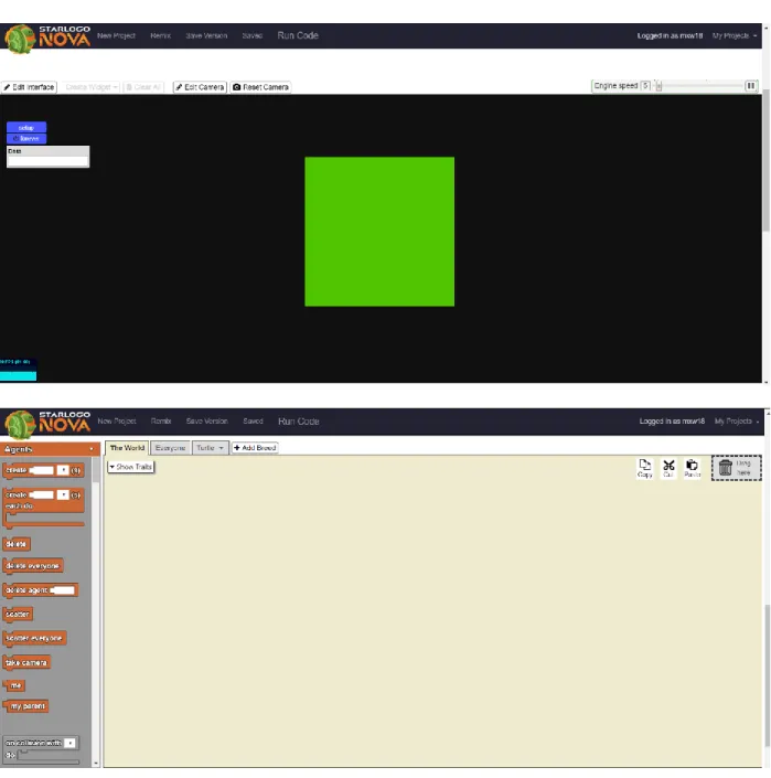
Nova is a web-based application that can be reached at slnova.org. It is used to program 3D simulations. After a user creates an account on StarLogo Nova, they can create a 3D simulation by making a project. Once a project is opened, a user interface containing a viewport and a workspace is presented to the

(10)

10

user [Figure 1]. These are the two main components of StarLogo Nova that a user engages with.

Figure 1: Top: StarLogo Nova viewport. Bottom: StarLogo Nova workspace.

The viewport is a window showing a 3D visualization of the current state of the simulation. The 3D visualization itself is called Spaceland. The viewport has several tools for interacting with Spaceland and providing user input to the underlying simulation. Among these tools are camera controls to manipulate the view of Spaceland and explore the 3D environment of the simulation.

(11)

11

The workspace is the area where a user programs the behavior of their simulation. Here, a program that defines the behavior of the simulation is constructed using blocks, components used to produce a graphical representation of a program, which we discuss further in Section 1.1.3. Users can compile and execute this program by pressing the “run code” button at the top of the web-page. Once the program in the workspace has been compiled and is running, the user can interact with the

simulation through the viewport.

To learn more about how to use the StarLogo Nova application, we suggest that the reader explore the resources page of the slnova.org website.

1.2.1 Agent-Based Simulation

Simulations in StarLogo Nova are agent-based. Agents are entities that possess several traits, including a position in 3D space. Users can add custom traits to an agent in addition to the existing traits built into StarLogo Nova. Agents are organized into breeds; a breed is similar to classes in other

programming languages. When a user creates a program in StarLogo Nova, they program the behavior of each breed, so that all agents of the same breed follow the same behavior. Users can create as many breeds as they desire, as well as any number of agents from each breed. The behavior of a breed can be programmed to alter the traits of other agents upon certain events, allowing agents to interact with one another. Breeds can even be programmed to create or destroy other agents upon certain events as well. The agent-based design of StarLogo Nova is what makes it well suited for computational modeling of complex systems. Agents are the individual components that make up a complex system.

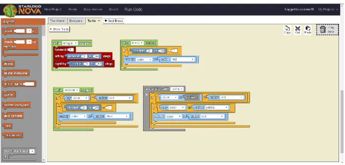
1.2.2 Block-Based Programming

StarLogo Nova does not make use of a written programming language or syntax. Instead,

programs are designed using a graphical representation in the workspace. The elements used to construct this graphical representation are called blocks. Control statements, intrinsic functions,

(12)

12

operators, event callbacks, and other elements commonly found in written programming languages are instead represented by individual blocks. A syntax exists dictating how blocks can be connected together or socketed inside one another in order to define a procedure [Figure 2]. The procedures constructed from blocks determine the behavior of agents, instantiate agents, and can respond to user input from the viewport, among other things. For more information on what blocks are available in StarLogo Nova and what they can do, we suggest that the reader visit the resources page of the slnova.org website.

Figure 2: A program in StarLogo Nova described graphically using blocks.

Using a block-based programming language gives StarLogo Nova several advantages over using a written programming language that are ideal for its intended target audience. Students using StarLogo

Nova in secondary school are novices when it comes to computer programming. Novices learning to

programming in a written programming language have to learn both the general concepts behind designing computer programs, such as computational thinking skills, and the syntax of the new language they are using to program. Having to remember the proper syntax used to write code leaves novices open to make mistakes that prevent their code from even compiling. With a block-based language, the blocks provide a graphical representation of the language’s syntax and enforce that syntax when a user

(13)

13

tries to connect blocks to form a program. Syntax errors cannot be made in block-based languages, and the user must recognize the syntax of the language rather than memorize it, which increases the learnability of the language by allowing novices to focus on learning programming concepts [Bau et al. 2017]. This increased learnability makes StarLogo Nova easier for novices to approach and allows them to spend more time learning computational thinking skills rather than the syntax of a particular

language, making StarLogo Nova more ideal for use in classroom settings.

1.3 Need for Additional Functionality

Although the agent-based design of StarLogo Nova is well suited for creating computational models, there are still limitations to the kinds of computational models that can be created. The agent-based design alone is not enough to implement models of some complex systems, may not provide enough capabilities to produce accurate models, or does not provide enough capabilities to make the implementation of the models feasible for secondary school students.

1.3.1 Computational Models That Are Difficult to Implement in StarLogo Nova

A thorough analysis of what kinds of complex systems are difficult to model in StarLogo Nova could be the research topic of an entire thesis, so we only discuss the kinds of complex systems that are difficult to model in StarLogo Nova that the work of this thesis makes possible to model with relative ease.

A complex system can be modeled in more than one way, depending upon what simplifications are made. Usually models of real-world complex systems must make simplifications because, in many cases, the components of a complex system can itself be seen as complex systems. For example, the predator-prey model discussed in Section 1.1.1uses individual predator and prey animals as the components of the complex system. However, an animal itself is a complex system comprised of cells,

(14)

14

and each cell is a complex system of biomolecules, and so forth. To say individual animals are the basic components of a predator-prey complex system is a simplification of the model.

A common case where simplifications are necessary are complex systems that involve modeling large environments. For example, if we want to model the erosion of a mountain due to runoff,

modeling the mountain with individual dirt particles as the components of the system would not be feasible. The choice of simplification is not obvious however. The mountain must be broken down into simpler components of some kind. The common approach to making a simplification of an environment is to section the environment into discrete parts that become basic components of the system. The mountain’s surface can be sectioned into separate parts in our example, and erosion can take place at individual parts of the surface, with neighboring parts possibly influencing one another. A basic

component that can be represented by an agent, for example, a rain drop that becomes runoff, can now interact with the simplified model of the mountain, and the mountain can update the section of surface area where the interaction took place. A solely agent-based design has difficultly implementing this kind of model. Using individual agents to model the sections of the mountain’s surface would be difficult because the surface agent would not only have to know how to interact with agents modeling the runoff, but also which agents are its neighboring surface sections which it influences. There is no straightforward way in an agent-based design to program an agent to interact with specific instances of other agents. If a user wants to make changes to the environment in a model to change the starting conditions of their simulation, this is also hard to do if the environment is comprised of agents, as a procedure must be created with blocks in order to produce a new arrangement of agents. Also, computational models in StarLogo Nova are visualized by depicting individual agents in 3D space, so there is also the question of how an environment such as the mountain can be properly visualized by a collection of individual agents. An adequate visualization might prove harder to implement than the model itself, especially for a secondary school student with limited knowledge and experience. A

(15)

15

different representation than agents must also be available to model large environments, one that is comprised of components that are spatially aware of one another, is configurable by the user, and has a visualization that is already suitable for its purpose.

A set of features to expand StarLogo Nova to support computational models involving large environments should provide an environment representation capable of interacting with agents in in a generalized way that can be used to model a wide variety of complex systems. It should also provide an adequate visualization of the environment, and should allow a user to configure the environment to meet the needs of their model and to change starting conditions. We will demonstrate how the work of this thesis meets these requirements revisiting the erosion complex system later in Section 6, showing how the new features we present in this thesis can be used to create several models for the complex system that can be implemented with ease.

1.3.2 Solutions in Previous Iterations of StarLogo

The predecessor to StarLogo Nova is StarLogo TNG, a desktop application. StarLogo Nova is very similar to StarLogo TNG and brings much of the same features to a web-based platform. StarLogo TNG addressed the issue of computational models that require a different representation of the environment aside from agents. In StarLogo TNG, an object called the Terrain represents the ground and is sub-divided into square sections called patches. These patches could be manipulated by both agents through blocks and by the user through an editor in order to change the shape of the Terrain [Figure 3]. The work of this thesis used the Terrain representation in StarLogo TNG as an inspiration and starting point to develop the Terrain representation that is now a part of StarLogo Nova. For those familiar with

StarLogo TNG, there are several features contributed by the work of this thesis that were not present in StarLogo TNG. The purpose of this thesis is not necessarily related to the goals that the designers of StarLogo TNG had, and so many design choices are made differently in the work of this thesis regarding

(16)

16

the Terrain. That being said, the work of this thesis does bring StarLogo Nova closer to the wider set of features and capabilities that its predecessor, StarLogo TNG, had.

Figure 3: Editable terrain from StarLogo Nova’s predecessor, StarLogo TNG.

2 Environment Representation

The environment in which StarLogo Nova simulations take place is a 3-dimensionsal space called The World. The World is a rectangular region bounded on six sides; agents in a simulation stay within this bounded region at all times. The positive z-axis is the up direction, with movement in the x and y axes being sideways. The World possesses a standard unit of measure, which we refer to as the world unit in later sections.

Aside from agents, The World contains one special object called the Terrain. Previously in

StarLogo Nova, the Terrain was a flat plane that served as a visualization for ground level [Figure 4].

(17)

17

move in the xy-plane. Agents could interact with the Terrain by drawing on it, changing its color locally underneath the agent.

The work of this thesis is to expand upon the functionality of the Terrain, making the Terrain a feature of the environment that agents can interact with and in turn can interact with the agents. Users should also be able to make changes to the Terrain themselves in order to setup a unique environment for agents to interact with that can serve their own purposes.

Figure 4: Previous terrain in StarLogo Nova; a simple visualization of the ground that has no impact on the simulation.

2.1 Terrain

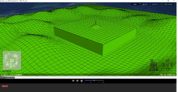
The Terrain is an object within The World that serves as a visualization for ground level in

StarLogo Nova simulations. However, ground level is no longer restricted to the z equals zero plane, as it

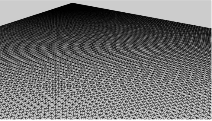
was in previous versions of StarLogo Nova. Instead of a plane, the Terrain is now visualized by a triangle mesh.

A triangle mesh is an open or closed geometric surface approximated by a collection of triangles. These triangles are connected by sharing edges; an arbitrary shape is assembled from triangles by

(18)

18

connecting them in this manner [Figure 5]. For a more detailed explanation of triangle meshes, we refer the reader to [Foley 1994]. By using a triangle mesh, the terrain can be morphed from a plane into an arbitrary surface, allowing the height of the terrain at any point to vary in the z-dimension. Ground level can therefore change locally as an agent moves over the Terrain. The shape of the Terrain is

manipulated by manipulating the geometry of the individual triangles that comprise the Terrain, which can be done either by an agent or a user.

Figure 5: An example of a triangle mesh.

The Terrain now also serves as a spatial data store. Numerical data can be stored at discrete locations spread over the Terrain in the pattern of a regular grid. Data is stored under a name in a lookup table, allowing more than one numerical value to be stored at each grid point.

The Terrain can now be manipulated by agents in two ways, changing the geometry or shape by editing the underlying triangles in the triangle mesh, and writing data to the Terrain at the grid points. The Terrain in turn can manipulate the agents; agents walking along ground level follow the height of

(19)

19

the Terrain. Changing the height of the Terrain therefore affects how agents move about The World. Agents may also be programmed to act differently depending upon what data they read from the grid points on the Terrain, so the Terrain’s data store can directly affect the behavior of the agents. These features provide a mechanism for agents and their environment to interact with and influence one another.

2.2 Patches

Users and agents don’t interact with the entire Terrain. Instead, they interact with a local region. Patches are an organizational structure for subdividing the Terrain into discrete units that can be

manipulated by a user or agent. When an agent interacts with the Terrain, they only interact with a single patch. Similarly, when a user makes edits to the Terrain, they select patches to edit, with a single patch being the smallest element they can edit. Patches also serve as the grid points at which data is stored; each patch has a data store that an agent can read from and write to. Triangles within the Terrain’s triangle mesh are arranged such that they are contained within a unique patch. Triangles are assigned to the patch that they are contained in. When a patch’s geometry is manipulated, it is responsible for updating its triangles accordingly. Section 5 discusses more the relationship between patches and their underlying triangles, but for now we can think of patches as being the objects that are geometrically manipulated by agents and users.

The patches which the Terrain is subdivided into can be distinguished into one of two types, floor patches and wall patches. We discuss the difference between these two types in the following subsections.

2.2.1 Floor Patches

Floor patches are the patches that agents walk over when they traverse the Terrain. Any patch that has a visible cross section when looking down the z-axis is a floor patch. Floor patches are directly

(20)

20

manipulated by the user or by agents. Agents can read data from and store data at a floor patch. Both users and agents can directly manipulate the geometry of a floor patch as well.

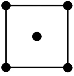
The Terrain is divided into floor patches such that when the Terrain is planar, the floor patches form a square grid. Each floor patch has four corner points and a center point. These five points serve as handles to manipulate the geometry of the floor patch [Figure 6]. To maintain an aligned grid of floor patches and preserve the location of the center of each floor patch, the corner and center points of each floor patch remain fixed in the x and y dimensions. This helps to preserve the boundaries of the The World, which typically match up with the outer edges of the Terrain. This also helps to maintain a sense of distance and makes floor patches a reliable unit of measure. Moving 20 patches left and then 20 patches right should bring you back to the same location, even if the Terrain changed shape during the movement. The center point of a floor patch also determines the spatial location of its data store from the perspective of the agents. Data stored at a particular location should not migrate to a new location due to Terrain changing shape. When a user or agent manipulates the geometry of a floor patch, only the z dimension is affected. By changing the z coordinate of the corner and the center points of one or more floor patches, the Terrain can be molded into a wide variety of shapes.

(21)

21

Figure 6: The location of the five points on a floor patch that serve as handles for manipulating the underlying triangle mesh.

2.2.2 Wall Patches

Manipulating the geometry of floor patches can result in discontinuities in the Terrain that appear as holes when viewed from the side. These discontinuities occur when a floor patch is

manipulated in such a way that one of its edges does not match up with the edge of an adjacent floor patch. A second type of patch exists to cover up these holes called wall patches. Wall patches cannot be directly manipulated by the user or by agents. They also do not possess the data stores that floor patches have. Instead, wall patches are manipulated indirectly. Wall patches automatically update to cover holes created by discontinuities and are hidden when discontinuities are not present [Figure 7]. Because the corners of each floor patch are fixed in the x and y dimensions, wall patches, as well as the discontinuities that they cover, do not have a visible cross section when looking down the z-axis. Therefore, any patch that does not have a visible cross section when looking down the z-axis is a wall patch. There is no interaction between agents and wall patches. Wall patches exist only for the purpose

(22)

22

of visualization so that the Terrain appears to be one solid entity without gaps.

Figure 7: The vertical sections are wall patches that adjust in order to cover up discontinuities that arise when the edges of neighboring floor patches do not agree.

2.3 Commands

Patches are manipulated by agents and by the user via commands. The geometric properties of patches (the underlying triangles) are not directly exposed to users or to agents. Instead, a set of commands exist that manipulate the geometry of one or more patches according to a procedure that acts on the corner and center points of floor patches. Individually, these commands make simple changes to the geometry of the Terrain, but when used together can result in complex results and can be a very expressive tool. Section 3 discusses the commands that are available to the user and Section 4 discusses the commands available to agents.

2.3.1 Undo/Redo

Most commands are recorded into a log of commands. By referencing this log, commands that manipulate the Terrain can be undone and redone via two special commands called undo and redo.

(23)

23

These function similarly to the undo and redo as found in many other software applications that provide an editor interface.

3 Terrain Editor

The Terrain Editor is a new system within StarLogo Nova that exposes a set of commands to the user that affect the geometry of the Terrain. The Terrain Editor is available to the user both during and outside of simulation, so that the user can make changes to the Terrain ahead of time or on the fly. In this section we discuss the user interface of the Terrain Editor and describe the commands that it exposes.

3.1 User Interface

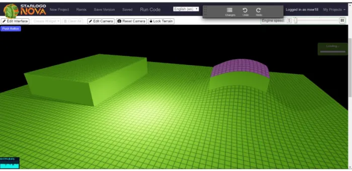
Here we only explain the key features of the user interface. Additional minor features can be found in the Appendix. The Terrain Editor can be activated in StarLogo Nova by pressing the “Edit Terrain” button located above Spaceland. Clicking “Lock Terrain” deactivates the Terrain Editor. When the Terrain Editor is active, black gridlines appear over the Terrain. These gridlines show the boundaries between individual floor patches. The Terrain Editor makes use of StarLogo Nova’s current camera control system in order to move around the user’s perspective and view the Terrain from different angles, which can be helpful during editing. The camera controls can be found in the Appendix.

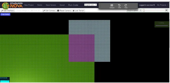
3.1.1 Selection

Commands can only be performed by the user on floor patches that are currently selected. Selecting floor patches is done using the left mouse button. By clicking with the left mouse button on an individual floor patch and then dragging, the user can select a rectangular region of floor patches. Releasing the left mouse button completes the selection. Selected patches appear highlighted in purple. The next command that is performed by the user will operate on the floor patches highlighted purple

(24)

24

within the selection. The selected region can extend past the edges of the Terrain, in which case virtual patches within the selection appear in cyan [Figure 8]. How selecting virtual patches affects the

command done by the user depends on which command was used.

Figure 8: A selection performed by the user in the terrain editor. Cyan patches are “virtual patches” outside of the terrain bounds.

3.2 Tools and Terrain Modification

Tools in the Terrain Editor allow the user to execute commands on the floor patches that they have selected. To distinguish between a tool and a command, a command is a procedure that operates on floor patches. A tool invokes a command with the proper arguments based on the user’s input. When a command takes an argument for elevating the height of the Terrain, tools provide those arguments in World units. In the following subsections, we give a qualitative description of the effect of each

command available to the user and give a high-level description of the algorithm used to provide that effect. We then explain the user interface controls of the corresponding tool that is used to execute the command. Tools make use of the mouse wheel and right mouse button, leaving the left mouse button available to use for selection.

(25)

25

3.2.1 Raise

Raise is a command that elevates every floor patch within a selection. Features of the Terrain within the selection are preserved, and a discontinuity is created around the edges of the selection that results in the formation of wall patches [Figure 9].

Figure 9: The raise command performed on both a flat and a curved region.

The algorithm for raise is simple. Raise iterates over each floor patch and increments the height of each point in the patches by a constant value, where the height value is given as an argument. Raise is additive, meaning that performing raise multiple times on the same selection is equivalent to

performing raise once with the sum of the height arguments.

The tool for raise makes use of the mouse wheel. Scrolling up repeatedly invokes raise, causing the selection to move up by one world unit with each scroll. Scrolling down also invokes raise, but with a negative height argument, causing the selection to move down one world unit with each scroll. If part of

(26)

26

the selection includes virtual patches, the virtual patches are ignored. The raise tool is activated by pressing ‘1’ on the keyboard.

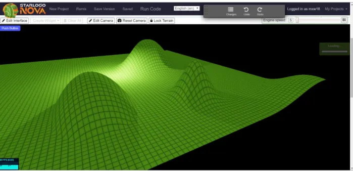
3.2.2 Mound

Mound is a command that elevates every floor patch within a selection, but does not create discontinuities and therefore does not result in the creation of wall patches. The floor patches are not elevated uniformly; instead each point in a floor patch is elevated based on its distance from the center of the selection. When applied to a flat region of the Terrain, this results in the formation of rounded geometry that resembles a hill. If the region is not flat, features of the Terrain within the selection are distorted by the curvature of the mound, and any wall patches that were previously visible will persist [Figure 10]. The curvature of the mound can be adjusted wider or skinnier.

Figure 10: The mound command. The width and tapering of the mound can be adjusted. The rear mound features default width and tapering.

The algorithm for mound uses a special height function to compute the height that each point in each floor patch should be elevated.

(27)

27 ∆𝑧 = 𝐴 cos (𝜋(𝑥 − 𝑥0) 𝑤 ) cos ( 𝜋(𝑦 − 𝑦0) ℎ ) [𝑚𝑎𝑥(1 − 𝛼, 0) + max(𝛼, 0) exp (−3 ( (𝑥 − 𝑥0)2 𝑤 + (𝑦 − 𝑦0)2 ℎ ))] 𝛼 = (2√(𝑥 − 𝑥0) 2 𝑤2 + (𝑦 − 𝑦0)2 ℎ2 ) 𝑝

The variables x and y are the coordinates of a point within a floor patch. The variables x0 and y0 are the

coordinates of the center of the selection. Variables w and h are the width and height of the selection. Variable A is the elevation that would occur at the center of the selection, the highest elevation output by the function. Variable p is an attenuation parameter that controls how quickly the elevation tapers off toward zero, effectively making the mound wider or skinnier.

The height function used by mound is an interpolation between a cosine term and a hybrid gaussian-cosine term. This can be seen by factoring in the cosine term and noting the α function to be the interpolation factor. The α function creates an elliptical interpolation between the two functions. The level sets of the α function are ellipses, where the center of the selection is the α=1 level set and the α=0 level set is inscribed in the boundaries of the selection. The max function ensures that the

interpolation factor does not go below zero in the area between the α=0 level set and the boundaries of the selection. This interpolation ensures a smooth transition between the cosine term near the center of the selection and the hybrid gaussian-cosine term near the boundaries.

There are two reasons for choosing this complicated height function over a simpler a cosine, gaussian, or hybrid gaussian-cosine function. Firstly, the shape of the cosine function creates a more well-rounded shape than either the gaussian function or the hybrid function but does not taper off at the edges of the selection. The gaussian function does taper off, and can be truncated to zero at the boundary without any noticeable visual artifacts. The hybrid function also successfully tapes off at the boundaries. An interpolation between the cosine and hybrid function produces a function that retains

(28)

28

the pleasing shape of the cosine function while also tapering off just in time near the selection

boundaries with minimal visual artifacts. The second reason for the use of the interpolation factor is that is gives us a degree of control over the shape of the mound that is easy to use. By introducing the attenuation parameter p, we can control how quickly the function transitions from cosine to the hybrid, effectively controlling how wide or skinny the mound is. We can even reproduce the shape of either the cosine or the hybrid by using a very large p or a p close to zero respectively.

The function above is computed at and added to the z coordinate of each corner point within each floor patch. For the center points, they are set to the average height of the corner points. This is done to prevent visual artifacts and to ensure that the result of the mound command is a smooth surface. Mound is additive, meaning that performing mound multiple times on the same selection is equivalent to performing mound once with the sum of the height arguments.

The tool for mound makes use of the mouse wheel and the right mouse button. Scrolling up with the mouse wheel repeatedly invokes mound, causing the selection to move up by one world unit at the center of the selection with each scroll. Scrolling down also invokes mound, but with a negative height argument, causing the selection to move down one world unit at the center of the selection with each scroll. By holding down the right mouse button and dragging left or right, the user can adjust the attenuation parameter p of the height function and adjust the shape produced by mound to be wider or skinnier. If the selection includes virtual patches, the virtual patches are taken into consideration when determining the value of the parameters x0, y0, w, and h of the height function, allowing for the creation

of partial mounds that do not taper off before reaching the edge of the Terrain. The mound tool is activated by pressing ‘2’ on the keyboard.

(29)

29

3.2.3 Level

Level is a command that sets the height of every point in every floor patch within the selection to the same value. It produces a flat plane within the selection and eliminates wall patches within the selection as well. It can also result in the creation of wall patches around the edges of the selection [Figure 11].

Figure 11: The level command. The top of the curved mound was made flat again and level with the raised structure on the left.

The algorithm for level is simple. Level iterates over each floor patch and sets the height of each point in the patches to the same constant value, where the height value is given as an argument. Level is not additive; performing level again on a selection completely overwrites the previous level command and produces a result equivalent to only the last level command executed.

The tool for level makes use of both the right click and the mouse wheel. Once a selection is made, right clicking on any floor patch will invoke level, passing the height of the minimum point within the right-clicked patch as the height argument. This results in every floor patch within the selection becoming level with the minimum point within the right-clicked floor patch. Scrolling the mouse wheel

(30)

30

up invokes level with one plus the height of the minimum point within the selection, allowing the user to adjust the height of a leveled region after the first invocation of level. Scrolling down similarly invokes level with the height of the minimum point minus one to lower the selection. If part of the selection includes virtual patches, the virtual patches are ignored. The level tool is activated by pressing ‘3’ on the keyboard.

3.2.4 Close Seams

Close seams is a command that removes all wall patches visible within and around the boundaries of a selection. Only the points along discontinuities in the Terrain are adjusted so that the minimal possible work is done to remove the wall patches [Figure 12].

Figure 12: Close seams command. Discontinuities between the mound and the level region on top of it are removed, forming a curved lip.

The algorithm for close seams iterates over all of the corner points within the selection. Because floor patches are aligned on a regular grid, each corner point overlaps with three other corner points from neighboring floor patches. The average height of the corner point and its three neighboring corner points is computed and the corner point is set to the average. A discontinuity exists if and only if

(31)

31

overlapping corner points do not share the same height, so this algorithm only modifies the selection where wall patches are visible.

The tool for close seams is simple. Once a selection is made, the user can right click anywhere in order to execute the command. Close seams is not additive; executing close seams again on a selection that no longer has visible wall patches results in no change. If part of the selection includes virtual patches, the virtual patches are ignored. The close seams tool is activated by pressing ‘4’ on the keyboard.

3.2.5 Ramp

Ramp is a command that creates a smooth, linear transition between the points along opposite edges of a selection. The transition is created in either the direction of the x-axis from left to right, or the direction of the y-axis from top to bottom [Figure 13]. Ramp is useful for joining regions of the Terrain at different heights.

Figure 13: The ramp command used to make connections between raised structures and the ground. Rightmost ramp created with the help of virtual patches.

(32)

32

The algorithm for ramp takes an argument that indicates whether the linear transition should be made in the direction of the x or the y axis. If in the x-axis direction, the algorithm loops over rows of floor patches within the selection that are aligned in the x direction. If in the y-axis direction, the algorithm loops over columns of floor patches within the selection that are aligned in the y dimension. In the case of transition in the direction of the x-axis, for each row of floor patches, the corner points just outside of the selection on the left and right side are linearly interpolated from left to right. This is done twice, separately for both the corner points along the bottom of the row and along the top [Figure 14]. Center points are set to the average z position of the four corner points around them. The

procedure is analogous for the y-axis direction.

Figure 14: An illustration of a horizontal linear transition computed over corner points by ramp. The bold patches are the floor patches inside the selection. The light patches are neighboring floor patches just outside the selection

The tool for ramp makes use of the right mouse button. Once a selection has been made, the user can right click anywhere to the left or to the right of the selection to create a linear transition in the direction of the x-axis from left to right. Clicking above or below the selection creates a linear transition in the direction of the y-axis from top to bottom. If part of the selection includes virtual patches and the virtual patches extend in the direction of the linear transition, then the linear transition transitions to

(33)

33

zero at the outermost edge of the virtual patches. The ramp tool is activated by pressing ‘5’ on the keyboard.

3.2.6 Copy

Copy is a command that replicates the geometry of the Terrain inside the selection at another location. It functions similarly to copy-and-paste as found in many other software applications that provide an editor interface.

The algorithm behind copy is simple. For every floor patch in the selection, the height of each point is written into a temporary buffer. The contents of the temporary buffer are then written to floor patches at a location specified as an argument.

The tool for copy makes use of the right mouse button. After a selection is made, right clicking on any floor patch makes that floor patch a starting reference. Once the starting reference is chosen, the selection changes into an orange placement guide. Moving the mouse moves the placement guide; the placement guide follows the same displacement from the original selection as the displacement of the mouse from the starting reference. Right clicking again copies the contents of the selection to the current location of the placement guide. If part of the selection includes virtual patches, then the value of zero is copied from the virtual patches. The copy tool is activated by pressing ‘6’ on the keyboard.

3.2.7 Move

Move is a command that is similar to copy. Move replicates the geometry of the Terrain inside the selection at another location and resets the original geometry to zero. It functions similarly to cut-and-paste as found in many other software applications that provide an editor interface.

The algorithm behind move is similar to copy as well. For every floor patch in the selection, the height of each point is written into a temporary buffer. The z position of every point in the floor patches

(34)

34

are then set to zero. Finally, contents of the temporary buffer are then written to floor patches at a location specified as an argument.

The tool for move functions exactly the same as the tool for copy. After a selection is made, right clicking on any floor patch makes that floor patch a starting reference. Once the starting reference is chosen, the selection changes into an orange placement guide. Moving the mouse moves the

placement guide; the placement guide follows the same displacement from the original selection as the displacement of the mouse from the starting reference. Right clicking again moves the contents of the selection to the current location of the placement guide. If part of the selection includes virtual patches, then the value of zero is copied from the virtual patches. The move tool is activated by pressing ‘7’ on the keyboard.

3.2.8 Stretch

Stretch is a command that scales the size of all patches uniformly. The Terrain becomes larger as a result of the scaling. It should be noted that, although the size of a floor patch becomes larger, world units remain the same. By default, floor patches are 1 world unit by 1 world unit. Stretch is used to change floor patches to an arbitrary size. Stretch is used to increase the size of the simulation

environment without increasing the number of patches in the Terrain. For example, if the size of a floor patch is currently 1x1 world units, and the stretch command is used to double the size of the Terrain, then the size of a floor patch will become 2x2 world units and an agent now has to move twice as far to cover the same number of floor patches. Stretch only affects the x and y dimensions of the patches, the z dimension is unaffected. This is because tools operate in the z dimension in terms of World units.

The algorithm for stretch takes a scale argument. The geometry of the entire Terrain is first written into a temporary buffer. Instead of multiplying the x and y positions of the points in every patch by a multiplicative factor, the position of each patch are computed from the scale argument in the same

(35)

35

manner as the initialization of patch position data. This is to prevent accumulation of numerical error and ensure that patches always have the exact same floating-point position when the same scale argument is passed. After scaling, the z positions of the geometry from the temporary buffer is written to the Terrain ensuring that the z dimension is not affected by stretch.

The tool for stretch makes use of the right mouse button. Because stretch targets all patches in the Terrain, the user cannot make a selection while the stretch tool is active. Holding down the right mouse button hides the Terrain and brings up an orange square guide indicating the overall scale of the Terrain. Dragging away from the center of the guide increases the scale of the Terrain, while dragging toward the center decreases the scale. Releasing the right mouse button invokes the stretch command to resize the Terrain to match the size of the guide. The stretch tool is activated by pressing ‘8’ on the keyboard.

3.2.9 Grow

Grow is a command that increases or decreases the number of patches in the Terrain. This results in the Terrain becoming larger or smaller. Grow adds to or takes away from the perimeter of the Terrain so that the Terrain maintains a square perimeter. By itself, grow can be used to make space for more Terrain content. Grow can also be used in combination with stretch to change the density of patches within the Terrain, allowing the user to create more detailed features or to increase the resolution of simulations where agents interact with the Terrain by increasing the density of the Terrain’s spatial data store and allowing agents to modify the geometry of a denser set of patches. When the Terrain is enlarged using grow, the Terrain’s current geometry is maintained at the center, and the new patches added to the perimeter are set uniformly to height zero. If the Terrain is made smaller, geometry at the perimeter of the Terrain is lost, while the rest of the geometry remains intact.

(36)

36

The algorithm for grow takes a width and height argument for new width and height of the Terrain in floor patches. Similar to stretch, the algorithm first copies the geometry of the Terrain into a temporary buffer, then frees up memory for the current Terrain patches and initializes the required amount for the new Terrain dimensions. The geometry in the temporary buffer is then written back to the center of the Terrain, with any geometry lying outside the new Terrain dimensions being lost. The width and height arguments determine how many patches are created and how they are arranged to form the new Terrain.

In practice, the same value is always used for both width and height to maintain a square Terrain. This limitation is enforced because it is not clear how certain other systems in StarLogo Nova should be updated to work with a non-square Terrain, such as the painting system that allows agents to draw on the Terrain. Design choices regarding such systems and their implementation are beyond the scope of this thesis, and non-square Terrain dimensions using grow is ready to be supported once those design choices have been addressed.

The tool for grow makes use of the right mouse button. Because grow affects the entire Terrain, the user cannot make a selection while the grow tool is active. Holding down the right mouse button hides the Terrain and brings up an orange grid indicating the size and patch resolution of the Terrain. Dragging away from the center of the grid increases the patch resolution of the Terrain, while dragging toward the center decreases the patch resolution. Releasing the right mouse button invokes the grow command to resize the Terrain to match the patch count of the grid. The grow tool is activated by pressing ‘9’ on the keyboard.

4 Agent-Terrain Interaction

Agents and the Terrain interact with one another in one of two ways. The first way is through agent movement. When an agent moves, its movement is influenced by the geometry of the Terrain.

(37)

37

The second way is through commands. There are commands available to agents that enable them to manipulate the geometry of the Terrain, which in turn influences their movement, and also commands that enable agents to exchange information with the Terrain. This section discusses these interactions in more detail.

4.1 Terrain Traversal

Agents in StarLogo Nova can move about The World using movement blocks. The movement blocks available to agents include the forward, backward, up, and down. The up and down blocks move the agent in the z dimension, while the forward and backward blocks move the agent in the x and y dimensions based on the agent’s heading, a property of the agent that determines which way it is facing in the xy-plane. In previous versions of StarLogo Nova, agents can move freely through The World with no influence from the environment. Moving an agent forwards or backwards would leave the agent at the same height. We introduce a new movement system to StarLogo Nova where moving forward or backwards moves the agent not only in the x and y dimensions, but in the z dimension as well. Movement in the z dimension is determined by the change in the height of the Terrain as the agent moves over it.

To implement this new movement system, we introduce a new property of the agent called altitude. Altitude represents the agent’s height above the surface of the Terrain. As an agent moves over the Terrain using the forward or backward block, its altitude remains the same, but its z position may change depending on the height of the Terrain beneath its current position [Figure 15]. A positive altitude means the agent is above the Terrain, while a negative altitude means the agent is below the Terrain. An altitude of zero means the agent is just on top of the Terrain. Moving with the up or down

(38)

38 blocks adjusts the altitude of the agent up or down.

Figure 15: The bear and the helicopter are in the same xy-position, following the slope of a mound as they move forward. The bear is at altitude zero, and the helicopter at a positive altitude above the terrain.

In order to define the altitude of an agent, we must define the height of the Terrain for any xy-position. In previous sections, we have mentioned that floor patches possess handles for manipulating their geometry called points. Points have a z coordinate value that determines the height of the floor patch at that point. However, we have not defined the height of a floor patch continuously in the areas between points. The height of the Terrain at any arbitrary xy-position is determined by the triangle mesh of the Terrain. We define it formally in the following way. For a position (x, y), the height of the Terrain at (x, y) is the z coordinate of the intersection between the triangle mesh and a line that passes through the coordinate (x, y, 0) perpendicular to the xy-plane [Figure 16]. The height of the Terrain is a piecewise linear function due to this definition.

(39)

39

Figure 16: An illustration of a ray perpendicular to the z=0 plane intersecting a triangle within a floor patch. The z coordinate of the point of intersection is the height of the Terrain at that location.

4.2 Terrain Modification

Several commands are available to agents to manipulate the geometry of the Terrain. Unlike the commands available to the user through the Terrain Editor, these commands target patches within a small, local area based on the agent’s xy-position. These commands are made available to agents through blocks.

In the following subsections we give a qualitative description of the effect of each command and give a high-level description of the algorithm used to provide that effect. In each of the following

subsections, the phrase “floor patch beneath the agent” refers to the floor patch directly beneath the agent’s position when looking down the negative z-axis; the agent’s position falls between the four borders of the floor patch when projected to the xy-plane. The phrase “volume preserving” means that a command, when given the same arguments, always adds the same amount of signed volume to the Terrain. For a volume preserving command, the signed volume added to the Terrain is also directly proportional to one or more of the command’s arguments. Neither the location of the agent, nor the

(40)

40

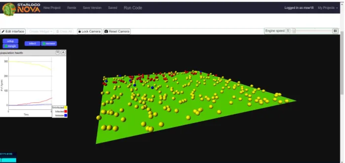
geometry of the Terrain affect the signed volume added by the command. The signed volume of the Terrain can be thought of as the volume between the triangle mesh of the Terrain and the z=0 plane, where the volume counts as positive where the Terrain’s height is positive and negative where the Terrain’s height is negative. This volume preserving property can be useful for simulations that require conservation of mass. Section 6 gives an example of such a simulation.

4.2.1 Build / Dig

Build is a command that takes a height argument and elevates the floor patch beneath the agent uniformly by that height. Build can create discontinuities in the Terrain that result in wall patches

becoming visible. Build is also volume preserving. It is similar to raise in its behavior.

The algorithm for build is simple. Each point of the floor patch beneath the agent is elevated by the height argument.

Dig is a counterpart command to build. It is equivalent to invoking build with a height argument multiplied by -1.

4.2.2 Yank / Stomp Grid

Yank grid is a command that takes a height argument and elevates the floor patch beneath the agent as well as the neighboring floor patches in a three by three grid [Figure 17]. Yank grid elevates the floor patches in a way so as not to create wall patches. Yank grid is volume preserving, adding the most volume to the floor patch beneath the agent and adding volume to the surrounding floor patches

(41)

41 following a discrete gaussian distribution.

Figure 17: An agent executing the yank grid command.

The algorithm for yank grid uses precalculated values from a template in order to determine the height that should be added to each point within the three by three grid affected by yank grid [Figure 18]. These template values are scaled by a height argument. The choice of template values ensures that wall patches do not get created by assigning the same value to overlapping corner points. The template values also ensure that the total signed volume added by yank grid is distributed in a discrete gaussian distribution. One fourth of the volume is distributed to the center floor patch, one eighth to the directly

(42)

42

adjacent floor patches, and one sixteenth to the corner floor patches.

Figure 18: The left illustration shows the template used for elevating each point within the 3x3 grid of floor patches. The decimals near each point are the fraction of the height argument that should be added to that point. The right illustration shows the breakdown of the signed volume distributed to each floor patch, a normalized, discrete gaussian kernel.

Stomp grid is a counterpart command to yank grid. It is equivalent to invoking yank grid with a height argument multiplied by -1.

4.2.3 Yank / Stomp

Yank is a command that takes a height argument and elevates the floor patches in the vicinity of the agent. The size of the vicinity is determined by a second width argument. Unlike yank grid, the peak of the elevation is not aligned with the center of any floor patch. It is aligned with the xy-position of the agent instead. Yank is a continuous version of yank grid. Like yank grid, yank does not result in the creation of wall patches. Yank is not volume preserving, the signed volume added to the Terrain is dependent on where the xy-position of the agent lies within the floor patch beneath the agent. As a compromise, yank does preserve the total height added to points in the Terrain and distributes that height in a gaussian distribution over the vicinity determined by the width argument. Height

(43)

43

preservation can be thought of as a discrete analog of volume preservation, with the points within a floor patch acting as the discrete sampling positions.

The algorithm for yank first computes the boundaries of a square region around the xy-position of the agent. The width of the square region is determined by the width parameter. A gaussian kernel function then computes a height displacement at every point that falls within the square region. The gaussian kernel is centered on the xy-position of the agent, and the standard deviation of the gaussian kernel is one third the width argument. After the height displacements have been computed by the gaussian kernel, they are reweighted so that their sum equals the height argument. This enforces the height preservation discussed in the previous paragraph.

4.3 Patch Data

Several commands are available to agents for reading from and writing to the data stores at each floor patch of the Terrain. These commands are made available to agents through blocks. Because these commands do not alter the geometry of the Terrain, they are not recorded by the undo/redo system. The following subsections use the phrase “floor patch beneath the agent” as described previously in Section 4.2.

4.3.1 Get / Set Attribute

Set attribute is a command for writing a numerical value to the data store of the floor patch beneath the agent. Set attribute takes a string argument in addition to the numerical value. The data store behaves similarly to a dictionary, so that if the string is not present in the data store, the numerical value is associated with the string. If the string is already present in the data store, then the numerical value overwrites the value that was previously associated with that string.

Get attribute is a command for reading a numerical value from the data store of the floor patch beneath the agent. Get attribute takes a string argument. As mentioned previously, the data store

(44)

44

behaves like a dictionary. If the string is present in the data store, then the last value associated with that string by set attribute is returned. If the string is not present in the data store, then zero is returned.

4.3.2 Interpolate Attribute

It is a common task to have to interpolate values between elements in a spatial data structure. Interpolate attribute is a command that provides this functionality. Interpolate attribute performs bilinear interpolation between the data stores of the four floor patches closest to the xy-position of the agent. The data stores are located at the center point of their respective floor patch. Interpolation is performed based on where the xy-position of the agent falls between the xy-positions of the center points of the four nearest floor patches. For those unfamiliar with bilinear interpolation, we refer the reader to [Press 1992].

5 Software Design and Implementation Details

The previous sections have described the new features provided by the work of this thesis as they appear to a StarLogo Nova user. In this section we discuss the software representation of the Terrain and the interface that it exposes to the rest of the StarLogo Nova application that make the new features possible. We also discuss the data representation of the Terrain’s state and the data structures used to organize and maintain that state. We also shed some light on how the Terrain’s state goes from data to the visualization seen by users on screen, and how users and agents are able to interact with that data.

5.1 Terrain Class

Following an object-oriented design pattern, the Terrain is represented by a class implemented in Javascript. In this section, we describe the key methods of the Terrain class and how they are used. By creating an instance of the Terrain class and making calls to the following methods, StarLogo Nova is

(45)

45

able to provide the features that have been described in Section 3 and Section 4. We also explain in this section the implementation of features that are managed internally by the Terrain class, namely the undo/redo system.

Some methods of the Terrain class make use of a different coordinate system than The World that uses the width of a patch as the unit of measure. We refer to the coordinate system of the Terrain as patch coordinates and the coordinate system of The World as world coordinates from now on. Patch coordinates are a two-dimensional coordinates system only defined in the xy-plane, unlike the three-dimensional world coordinates that are defined anywhere in space. Integral patch coordinates align with the at the center points of every floor patch. The bottom, leftmost floor patch is located at (0, 0), with the x patch coordinate increasing from left to right and the y patch coordinate increasing from bottom upwards.

5.1.1 Methods and Interface

Public Interface:

toggleEditMode (enable)

enable: True to enable, false to disable. Enables or disables the Terrain Editor.

setMouseCommand (command)

command: Bitwise OR of flags representing different commands.

Activates the tools indicated by the command argument and disables all other tools. setWheelSpeed (sensitivity)

sensitivity: New sensitivity of the mouse wheel.

Changes the sensitivity of the mouse wheel for tools in proportion to the sensitivity argument. select (left, bottom, right, top)

left: Left boundary of a selection, inclusive. Integer patch coordinate.

bottom: Bottom boundary of a selection, inclusive. Integer patch coordinate. right: Right boundary of a selection, inclusive. Integer patch coordinate. top: Top boundary of a selection, inclusive. Integer patch coordinate.

(46)

46

Marks a rectangular region of floor patches the selection to be manipulated by the next command from the user in the Terrain Editor.

clearSelection ()

Sets a null selection in the Terrain Editor. patchToWorld (patch_x, patch_y)

patch_x: Horizontal coordinate in patch coordinate space. Floating point. patch_y: Vertical coordinate in patch coordinate space. Floating point.

Converts patch coordinates to world coordinates and returns them as a length two array. worldToPatch (world_x, world_y)

world_x: Horizontal coordinate in world coordinate space. Floating point. world_y: Vertical coordinate in world coordinate space. Floating point.

Converts world coordinates to patch coordinates and returns them as a length two array. getHeightAt (x, y)

x: Horizontal coordinate in patch coordinate space. Floating point. y: Vertical coordinate in patch coordinate space. Floating point.

Computes the height of the Terrain at an arbitrary point using barycentric interpolation. raise (height, x, y, right, top, logHistory)

height: Distance to elevate in world units.

x: Left boundary of a selection, inclusive. Integer patch coordinate. y: Bottom boundary of a selection, inclusive. Integer patch coordinate. right: Right boundary of a selection, inclusive. Integer patch coordinate. top: Top boundary of a selection, inclusive. Integer patch coordinate. logHistory: True to log command with the undo/redo system. False to omit.

Performs the raise command on the region defined by x, y, right, and top. If right or top is null, perform the command on the patch specified by x, y. If x or y is null, perform the command on the current selection.

mound (amplitude, attenuation, x, y, right, top, logHistory) amplitude: Distance to elevate in world units.

Performs the mound command on the region defined by x, y, right, and top. If right or top is null, perform the command on the patch specified by x, y. If x or y is null, perform the command on the current selection.

(47)

47 level (x, y, right, top, logHistory)

Performs the level command on the region defined by x, y, right, and top. If right or top is null, perform the command on the patch specified by x, y. If x or y is null, perform the command on the current selection.

closeSeams (method, x, y, right, top, logHistory)

method: A constant indicating what method should be used to remove wall patches, joining floor patches at the minimum, maximum, or average of their overlapping points.

Performs the close seams command on the region defined by x, y, right, and top using the method indicated by the method argument to seal seams. If right or top is null, perform the command on the patch specified by x, y. If x or y is null, perform the command on the current selection.

ramp (direction, x, y, right, top, logHistory)

direction: A constant indicating whether the direction of the ramp should be left to right or top to bottom.

Performs the ramp command on the region defined by x, y, right, and top in the direction indicated by the direction argument. If right or top is null, perform the command on the patch specified by x, y. If x or y is null, perform the command on the current selection.

copy (dst_x, dst_y, x, y, right, top, logHistory)

dst_x: Horizontal coordinate in patch coordinate space. Integer. dst_y: Vertical coordinate in patch coordinate space. Integer. x: Left boundary of a selection, inclusive. Integer patch coordinate. y: Bottom boundary of a selection, inclusive. Integer patch coordinate. right: Right boundary of a selection, inclusive. Integer patch coordinate. top: Top boundary of a selection, inclusive. Integer patch coordinate. logHistory: True to log command with the undo/redo system. False to omit.

Custom and interactive environments in StarLogo Nova for computational modeling

Custom and Interactive Environments in StarLogo Nova

for Computational Modeling

by Malcolm X. Wetzstein

B.S., Computer Science and Engineering,

Massachusetts Institute of Technology (2019)

Submitted to the

Department of Electrical Engineering and Computer Science

in Partial Fulfillment of the Requirements for the Degree of

Master of Engineering in Electrical Engineering and Computer Science

at the

Massachusetts Institute of Technology

August 2019

© Massachusetts Institute of Technology 2019. All rights reserved.

Custom and Interactive Environments in StarLogo Nova

for Computational Modeling

by Malcolm X. Wetzstein

August 23

, 2019

In partial Fulfillment of the Requirements for the

Degree of Master of Engineering in

Electrical Engineering and Computer Science

Abstract

Thesis Supervisor: Eric Klopfer

Title: Professor

Table of Contents

List of Figures

1

Introduction

1.1

Purpose of StarLogo Nova

1.2

What is StarLogo Nova?

1.2.1 Agent-Based Simulation

1.2.2 Block-Based Programming

1.3

Need for Additional Functionality

1.3.1 Computational Models That Are Difficult to Implement in StarLogo Nova

1.3.2 Solutions in Previous Iterations of StarLogo

2

Environment Representation

2.1

Terrain

2.2

Patches

2.2.1 Floor Patches

2.2.2 Wall Patches

2.3

Commands

2.3.1 Undo/Redo

3

Terrain Editor

3.1

User Interface

3.1.1 Selection

3.2

Tools and Terrain Modification

3.2.1 Raise

3.2.2 Mound

3.2.3 Level

3.2.4 Close Seams

3.2.5 Ramp

3.2.6 Copy

3.2.7 Move

3.2.8 Stretch

3.2.9 Grow

4

Agent-Terrain Interaction

4.1

Terrain Traversal

4.2

Terrain Modification

4.2.1 Build / Dig

4.2.2 Yank / Stomp Grid

4.2.3 Yank / Stomp

4.3

Patch Data

4.3.1 Get / Set Attribute

4.3.2 Interpolate Attribute

5

_{, 2019}