Coverage optimization using a single satellite orbital figure-of-merit

Coverage Optimization Using a Single Satellite Orbital Figure-of-Merit by

John L. Young III B.S. Aerospace Engineering United States Naval Academy, 2001

SUBMITTED TO THE DEPARTMENT OF AERONAUTICS AND ASTRONAUTICS IN PARTIAL FULFILLMENT OF THE REQUIREMENTS OF THE DEGREE OF

MASTER OF SCIENCE IN AERONAUTICS AND ASTRONAUTICS

AT THE MASSACHUSETTS _INSTITUTE

MASSACHUSETTS INSTITUTE OF TECHNOLOGY OF TECHNOLOGY

June 2003 NL 0 52

J

@ 2003 John L. Young III. All Rights Reserved LIBRARIES The author hereby grants to MIT permission to reproduce and distribute publicly paper

and electronic copies of this thesis document in whole or in part.

Signature of Author

Department of Aeronautics and Astronautics May 23, 2003 Certified by

David W. Carter Technical Staff, The Charles Stark Draper Laboratory Thesis Supervisor Certified by_

John E. Draim Captain, USN (ret) Thesis Advisor Certified by

Paul J. Cefola Technicistaff, The MIT Lincoln Laboratory Lecturer, Department of Aeronautics and Astronautics Thesis Advisor

Accepted by E

H.N. Slater Professor of Aeronautics and Astronautics Chair, Committee on Graduate Students

MILbraries

DISCLAIMER NOTICE

The accompanying media item for this thesis is available in the MIT Libraries or Institute Archives.

Coverage Optimization Using a Single Satellite Orbital Figure-of-Merit By

John L. Young III

Submitted to the Department of Aeronautics and Astronautics on May 23, 2003, in partial fulfillment of the requirements for the

Degree of Master of Science In Aeronautics and Astronautics Abstract

A figure-of-merit for measuring the cost-effectiveness of satellite orbits is introduced and applied to various critically inclined daily repeat ground track orbits. The figure-of-merit measures orbit performance through the coverage time provided over a specified point or region on the ground. This thesis primarily focuses on coverage to a ground station, however coverage to a region is briefly examined. The selected repeat ground track orbits are optimized to maximize the coverage provided by varying the orbit's argument of perigee and longitude of ascending node. Several known orbits were reproduced as a result of this coverage optimization. The figure-of-merit measures the cost of the orbit by the launch cost in AV to attain the mission orbit. The launch AV is calculated using a series of analytic formulas.

Trends in the figure-of-merit are investigated with respect to repeat ground track pattern, ground station location, orbit eccentricity, and minimum elevation angle. Using the proposed figure-of-merit, various repeat ground track orbits are examined and compared to draw conclusions on the cost-effectiveness of each orbit. This figure-of-merit has potential for use by satellite system designers to compare the cost-effectiveness of different orbits to determine the optimal orbit for a single satellite and by extension, a constellation of satellites.

Technical Supervisor: Dr. David W. Carter

Title: Member of the Technical Staff, C.S. Draper Laboratory, Inc. Thesis Advisor: Dr. Paul J. Cefola

Title: Member of the Technical Staff, MIT Lincoln Laboratory Thesis Advisor: Captain John E. Draim, USN (ret)

ACKNOWLEDGEMENTS May 23, 2003

I would first like to thank the Charles Stark Draper Laboratory for the opportunity and funding to pursue my Masters Degree these past two years. I would also like to thank my thesis advisor, Dr. David Carter, for taking me on as a student. If it were not for him, I would probably still be searching for a research topic. I gained a wealth of knowledge from our numerous meetings and discussions. It was also a pleasure working with Dr. Paul Cefola, from whom I have learned a great deal. He was right when he told me that I was going to be playing with the 'big dogs,' and I am happy that I had to opportunity to do so. The insight from Captain John Draim, USN (ret) was also instrumental in this thesis. It is always great working with another Annapolis grad. Hopefully I will be able accomplish some of the great things that he has done in his career, both in and out of the Navy. This thesis would not have been possible without the help from all three of my advisors. Countless hours were spent on the phone with them reviewing both my work and my writing. I am also grateful for their support in writing the AAS Paper this past February. It was an extremely valuable experience and I can't complain about Puerto Rico.

Thanks also goes to Jeff Cipolloni of Draper Laboratory for his time with all of my computer questions and problems.

I would also like to thank the Draper Fellows I have worked with my time here. Eric, we first met as roommates 2/c year in Annapolis. Who would have thought that we'd end up working down the hall from each other two years later? Thanks for all your help these past two years and I wish you and Emily the best of luck in the future. Andrew, what can I say? We've had a lot of fun here, both in the office and out of it. Thanks (I think) for introducing me to the addicting habit we call golf. We've had some good times on the course- in the snow, pouring rain, and sweltering heat. It's a good thing there was another crazy person to go play when no one else would. Good luck at Power School and I'm sorry I won't be down there to enjoy it with you. Stephen, what are we going to do without the great state of Massachusetts? I know you thought I was crazy and didn't think I'd be able to go NFO, but thanks for humoring me for over a year. It is too bad I won't be able to hang out with both you and Andrew down in Charleston. To the rest of the Fellows, Chris G., Hon-Fai, Stuart, Ed, Barry, Luke, Corbin, Chris J., Daryl, and Keith, thanks for all of the interesting lunch time discussions. Ed, I'll see you down in Pensacola in a year.

Finally I would like to thank my family for their support throughout the years. Without it, I would have never gotten this far. Thank you.

This thesis was prepared at The Charles Stark Draper Laboratory, Inc., under internal Independent Research and Development Project 0305043.

Publication of this thesis does not constitute approval by Draper or the sponsoring agency of the findings or conclusions contained herein. It is publikhed for the exchange and stimulation of ideas.

Table of Contents

1 Introdu ction ...

15

1.1 Thesis Objective ... 15

1.2 Figure-of-M erit...15

1.3 Thesis Sum m ary ... 17

2 B ackground ...

19

2.1 Chapter Overview ... 19

2.2 Cost-Effectiveness M etrics... 19

2.2.1 Cost Per Billable M inute... 19

2.2.2 Cost Per Billable TI M inute... 20

2.3 Satellite Constellation Perform ance ... 21

2.3.1 Revisit Tim e ... 21

2.3.2 Coverage Tim e ... 22

2.4 Constellation D esign... 22

2.4.1 R .D . LU ders... 22

2.4.2 R . L. Easton and R. Brescia... 23

2.4.3 John W alker...24 2.4.4 D avid Beste...24 2.4.5 A rthur Ballard... 25 2.4.6 John Draim ... 27 2.4.7 Thom as Lang ... 30 2.4.8 John H anson ... 30

3 M ethodology ...

31

3.2 Repeat Ground Track Orbits ... 31

3.3 Repeat Ground Track Orbit Calculation ... 34

3.4 Coverage Function ... 36

3.4.1 CoverageTim e.m ... 37

3.4.2 COEUpdate.m ... 37

3.4.3 CalcD eltaElA ngle.m ... 38

3.4.4 COEtoPosition.m ... 40

3.5 Function Testing ... 41

3.6 Coverage Plots...41

3.7 N onlinear Optim ization / M atlab "fm incon" function ... 43

3.8 Delta-V Calculation... 43

3.9 Figure-of-M erit Calculation ... 47

4 R esults ...

49

4.1 Chapter Overview ... 49

4.2.1 Orbits Examined... 49 4.2.2 Contour Plots ... 50 4.2.3 Optimal Orbits ... 55 4.2.3.1 Tundra/Sirius Orbit... 55 4.2.3.2 M olniya Orbit ... 58 4.2.3.3 COBRA Orbit ... 61 4.2.3.4 Ellipso-Borealis Orbit... 63 4.3 Delta-V Results...66 4.4 FOM Results...67 4.4.1 Contour Plots ... 67

4.4.2 Repeat Ground Track Comparisons ... 73

5 Conclusions...

77

6 Future W ork...

81

References ...

85

Appendix A: Figure-of-Merit Analysis Code ...

93

Appendix B: Coverage, Delta-V and Figure-of-Merit Results...99

Appendix C: Figure-of-M erit Contour Plots...

113

Appendix D: Repeat Ground Track Pattern Comparison ...

127

Appendix E: Coverage to a Region ...

135

E. 1 M ethodology ... 135

E .2 R esu lts ... 137

E.2.1 Coverage Plots ... 137

E.2.2 Figure-of-M erit Results...151

E.2.3 Repeat Ground Track Comparison...152

E.3 M atlab Code ... 154

List of Figures

Figure 2.1: Latitude Bounded Regions Examined by LUders ... 23

Figure 2.2: Earth-Centered Half-Cone-Angle [35] ... 25

Figure 2.3: "Rosette" Constellation as Viewed From the North Pole [36] ... 26

Figure 2.4: Ground Track and Coverage Plot for Draim's Three Satellite Constellation [38]...28

Figure 2.5: Draim COBRA "Teardrop" Array [42]... 29

Figure 3.1: Coverage Function Subroutines... 36

Figure 3.2: Geometry in the Elevation Angle Calculation ... 40

Figure 4.1: Contour Plot of Coverage, Low Latitude Ground Station ... 51

Figure 4.2: 3-D Contour Plot of Coverage, Low Latitude Ground Station ... 52

Figure 4.3: Ground Track Corresponding to Optimized Orbit for Coverage ... 53

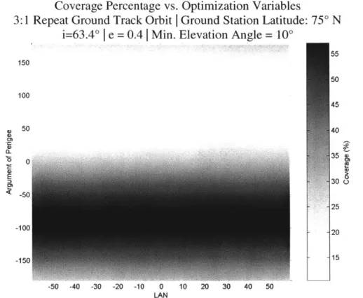
Figure 4.4: Contour Plot of Coverage- High Latitude Ground Station ... 54

Figure 4.5: 3-D Contour Plot of Coverage- High Latitude Ground Station ... 54

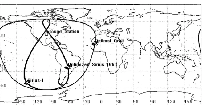
Figure 4.6: STK Ground Track Comparison for Sirius-I Orbit and Optimized Orbit ... 56

Figure 4.7: Leaning Soviet Molniya Ground Tracks [72]... 59

Figure 4.8: STK Ground Track Comparison for a Typical Molniya Orbit and Optimized Orbit...60

Figure 4.9: C ontour Plot of C overage ... 61

Figure 4.10: STK Ground Track Comparison for a Typical COBRA Orbit and Optimized Orbit ... 62

Figure 4.11: C ontour Plot of C overage ... 63

Figure 4.12: STK Ground Track Comparison for a Typical Ellipso-Borealis Orbit and Optimized Orbit ... 64

Figure 4.13: C ontour Plot of C overage ... 65

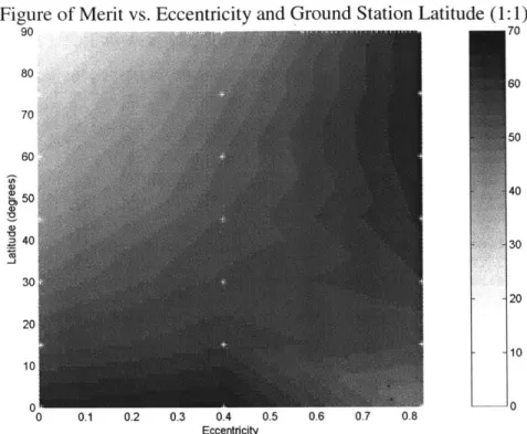
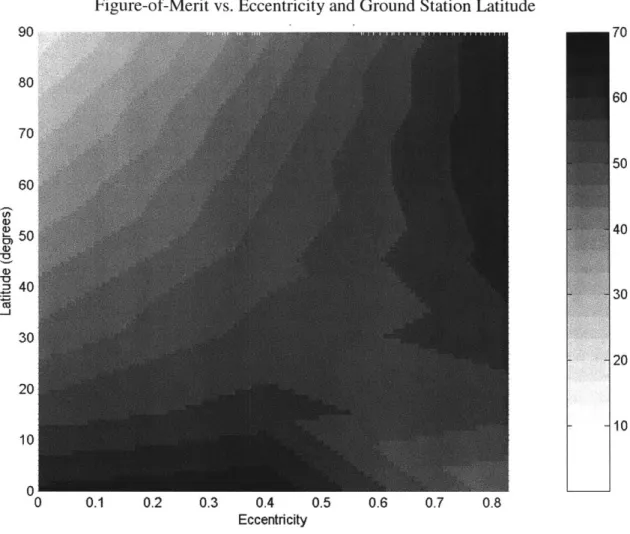
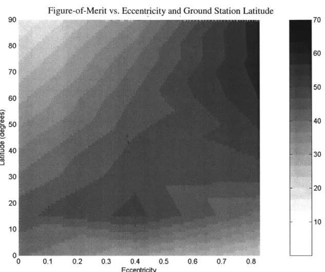
Figure 4.14: Figure-of-M erit Contour Plot ... 69

Figure 4.15: Figure-of-M erit Contour Plot ... 69

Figure 4.16: Figure-of-M erit Contour Plot ... 70

Figure 4.17: Figure-of-M erit Contour Plot ... 70

Figure 4.18: Figure-of-Merit Contour Plot (21 Data Points) ... 72

Figure 4.19: Figure-of-Merit Contour Plot (35 Data Points) ... 72

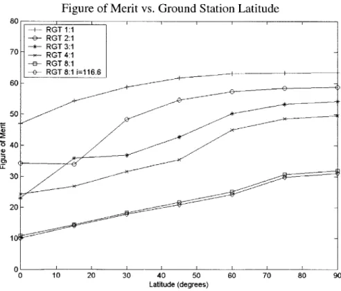
Figure 4.20: Figure-of-Merit Comparison for Varying Repeat Ground Track Patterns (e=0)...74

Figure 4.21: Figure-of-Merit Comparison for Varying Repeat Ground Track Patterns (e=0.4)...75

Figure 4.22: Figure-of-Merit Comparison for Varying Repeat Ground Track Patterns (e = max)... 75

Figure A .1: M atlab C ode Flow C hart...95

Figure C.1: Figure-of-Merit Contour Plot- 1:1 Repeat Ground Track Orbit, Minimum Elevation Angle: 10 . 114 Figure C.2: Figure-of-Merit Contour Plot- 1:1 Repeat Ground Track Orbit, Minimum Elevation Angle: 300. 115 Figure C.3: Figure-of-Merit Contour Plot- 2:1 Repeat Ground Track Orbit, Minimum Elevation Angle: 100 116

Figure C.4: Figure-of-Merit Contour Plot- 2:1 Repeat Ground Track Orbit, Minimum Elevation Angle: 300 .117 Figure C.5: Figure-of-Merit Contour Plot- 3:1 Repeat Ground Track Orbit, Minimum Elevation Angle: 10 .118 Figure C.6: Figure-of-Merit Contour Plot- 3:1 Repeat Ground Track Orbit, Minimum Elevation Angle: 300 .119 Figure C.7: Figure-of-Merit Contour Plot- 4:1 Repeat Ground Track Orbit, Minimum Elevation Angle: 100 .120 Figure C.8: Figure-of-Merit Contour Plot- 4:1 Repeat Ground Track Orbit, Minimum Elevation Angle: 300 .121 Figure C.9: Figure-of-Merit Contour Plot- 8:1 Repeat Ground Track Orbit, Minimum Elevation Angle: 10 .122

Figure C. 10: Figure-of-Merit Contour Plot- 8:1 Repeat Ground Track Orbit, Minimum Elevation Angle: 300 123 Figure C. 11: Figure-of-Merit Contour Plot- 8:1 Repeat Ground Track Orbit, i= 116.60, Minimum Elevation A n g le : 10 . ... 12 4 Figure C. 12: Figure-of-Merit Contour Plot- 8:1 Repeat Ground Track Orbit, i=116.60, Minimum Elevation A n g le : 30 ... 12 5

Figure D. 1: Figure-of-Merit Comparison for Varying Repeat Ground Track Patterns (e=0, Min. Elevation Angle = 100 ) ... 12 8 Figure D.2: Figure-of-Merit Comparison for Varying Repeat Ground Track Patterns (e=0, Min. Elevation Angle

= 3 00 ) ... 12 9 Figure D.3: Figure-of-Merit Comparison for Varying Repeat Ground Track Patterns (e=0.4, Min. Elevation A n g le = 10 0)... 13 0 Figure D.4: Figure-of-Merit Comparison for Varying Repeat Ground Track Patterns (e=0.4, Min. Elevation A n g le = 3 00 )... 13 1 Figure D.5: Figure-of-Merit Comparison for Varying Repeat Ground Track Patterns (e=max, Min. Elevation A n g le = 100)... 13 2 Figure D.6: Figure-of-Merit Comparison for Varying Repeat Ground Track Patterns (e=max, Min. Elevation A ng le = 300 )... 13 3

Figure E. 1: Geometry of Satellite Coverage ... 136

Figure E. 2: Selected Points on Boundary of Region (Continental U.S.)... 137

Figure E.3: Regional Coverage Contour Plot... 139

Figure E.4: Regional Coverage Contour Plot... 139

Figure E.5: Regional Coverage Contour Plot... 140

Figure E.6: Regional Coverage Contour Plot... 140

Figure E.7: Regional Coverage Contour Plot... 141

Figure E.8: Regional Coverage Contour Plot... 141

Figure E.9: Regional Coverage Contour Plot... 142

Figure E.10: Regional Coverage Contour Plot... 142

Figure E. 11: Regional Coverage Contour Plot... 143

Figure E.13: Regional Coverage Contour Plot... 144

Figure E. 14: Regional Coverage Contour Plot... 144

Figure E. 15: Regional Coverage Contour Plot... 145

Figure E. 16: Regional Coverage Contour Plot... 145

Figure E.17: Regional Coverage Contour Plot... 146

Figure E.18: Regional Coverage Contour Plot... 146

Figure E. 19: Regional Coverage Contour Plot... 147

Figure E. 20: Regional Coverage Contour Plot... 147

Figure E.21: Regional Coverage Contour Plot... 148

Figure E.22: Regional Coverage Contour Plot... 148

Figure E.23: Regional Coverage Contour Plot... 149

Figure E.24: Regional Coverage Contour Plot... 149

Figure E.25: Regional Coverage Contour Plot... 150

Figure E.26: Regional Coverage Contour Plot... 150

Figure E.27: Repeat Ground Track Orbit Comparison (100 Minimum Elevation Angle) ... 153

List of Tables

Table 2.1: Orbital Elements in a Draim Constellation [37]... 27

Table 3.1 Coverage Function Test Cases (Epoch: 01 January 2000)...41

Table 3.2 Comparison of Calculated Delta-V Values with Delta-V Examples ... 46

Table 4.1: Orbital Elem ents for Optim ized Orbit... 53

Table 4.2: Orbit Elements for Sirius-I and Optimized Orbits for a Ground Station at (36.5' N, 96.5' W, 0 km), M inim um E levation A ngle: 10 ... 56

Table 4.3: Comparison of Sirius and Optimal Orbit Coverage Times Based on Minimum Elevation Angle...57

Table 4.4: 1:1 Repeat Ground Track Orbit Optimizations, e = 0.8297 ... 57

Table 4.5: 1:1 Repeat Ground Track Orbit Optimizations: e = 0.2635...58

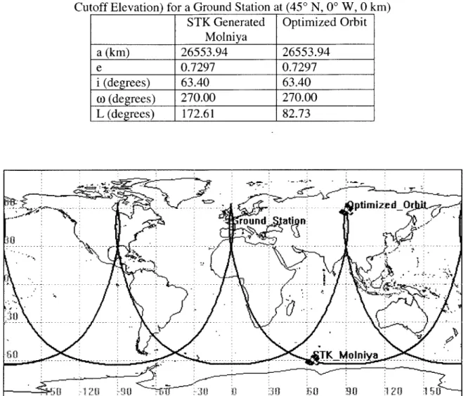
Table 4.6: Orbit Elements for an STK Generated Molniya Orbit and Optimized Orbit (100 Cutoff Elevation) for a Ground Station at (45 N, 0 W, 0 km)... 60

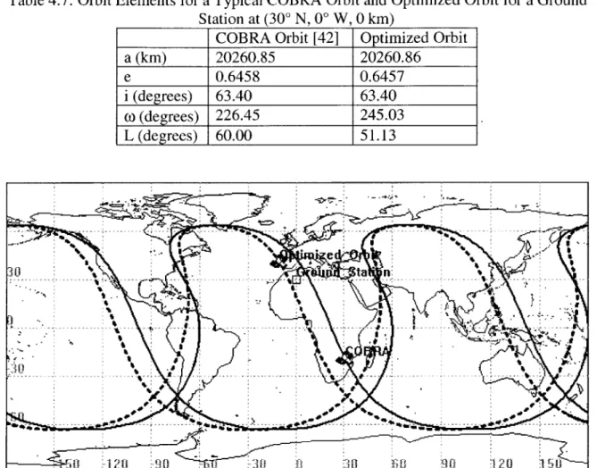
Table 4.7: Orbit Elements for a Typical COBRA Orbit and Optimized Orbit for a Ground Station at (300 N, 00 W , O k m ) ... ... 6 2 Table 4.8: Orbit Elements for a Typical Ellipso-Borealis Orbit and Optimized Orbit For a Ground Station at (30 N , 0 W , O km )... 64

Table 4.9: Coverage Time Per Day (%) vs. Ground Station Latitude ... 66

T able 4.10: A V C alculations (m /s)...67

Table B. 1: 1:1 Repeat Ground Track Orbit Results (Minimum Elevation Angle: 100, i=63.40_{)... 100}

Table B.2: 1:1 Repeat Ground Track Orbit Results (Minimum Elevation Angle: 300, i=63.40)... 101

Table B.3: 2:1 Repeat Ground Track Orbit Results (Minimum Elevation Angle: 10', i=63.40)... 102

Table B.4: 2:1 Repeat Ground Track Orbit Results (Minimum Elevation Angle: 30', i=63.40)... 103

Table B.5: 3:1 Repeat Ground Track Orbit Results (Minimum Elevation Angle: 10', i=63.40) ... 104

Table B.6: 3:1 Repeat Ground Track Orbit Results (Minimum Elevation Angle: 300, i=63.40)... 105

Table B.7: 4:1 Repeat Ground Track Orbit Results (Minimum Elevation Angle: 100, i=63.40)... 106

Table B.8: 4:1 Repeat Ground Track Orbit Results (Minimum Elevation Angle: 300, i=63.40_{) ... 107}

Table B.9: 8:1 Repeat Ground Track Orbit Results (Minimum Elevation Angle: 100, i=63.40)... 108

Table B. 10: 8:1 Repeat Ground Track Orbit Results (Minimum Elevation Angle: 300, i=63.40)... 109

Table B. 11: 8:1 Repeat Ground Track Orbit Results (Minimum Elevation Angle: 100, i=1 16.60)... 110

Table B.12: 8:1 Repeat Ground Track Orbit Results (Minimum Elevation Angle: 30', i= 116.60)... I11 Table E.1: Coverage, Delta-V and Figure-of-Merit Results (Min. Elevation Angle 10')... 151

1 Introduction

1.1 Thesis Objective

Satellites in Geostationary orbit (GEO) are extremely useful by providing 24 hour coverage to large regions of the Earth. Cost-effective alternatives to the GEO satellite are desirable due to high satellite and launch costs, as well as limited space in the Geostationary Belt. Constellations of satellites in low-Earth orbit (LEO), medium-Earth orbit (MEO) or

highly elliptical orbit (HEO) can be used effectively in communications systems and have

potential for providing excellent performance with lower cost than Geostationary satellites.

A metric that can be used by satellite designers to compare the cost-effectiveness of

different orbits would provide a valuable way to determine the optimal orbit for a single satellite and by extension, a constellation. This thesis investigates and expands the of-merit for single-satellite orbits proposed by Captain John Draim, USN (ret) [1]. The figure-of-merit examines the cost-effectiveness of the satellite's orbit applied from the standpoint of coverage, coupled with the launch cost of the satellite. The figure-of-merit was initially developed to apply to communications satellite systems, however it can be tailored to suit other applications. Orbits examined in this study are restricted to daily repeat ground track orbits which are critically inclined at either 63.4' or 116.6'.

1.2 Figure-of-Merit

The non-dimensional orbital figure-of-merit, J, examines the coverage time versus the launch cost in AV. The premise behind this metric is that in general, one can achieve better coverage for satellites placed in higher orbits, but the cost in AV also increases. For example, a satellite in Geostationary orbit will provide continuous coverage to the ground, but the launch cost in AV to attain the orbit is high. Therefore, a lower orbit with less coverage, but also a lower AV might offer an acceptable alternative.

In this thesis, the figure-of-merit is defined as:

T(a,e,i,Q,w,M)

where T is a measure of the average coverage time per day in seconds over the interval [to, t] where t - to is the repeat period. The orbit elements a, e, i, d, CO, and M correspond to time to. The quantity AV is the velocity increment in m/s required to attain the satellite's mission orbit from a launch beginning at the Earth's surface. The constant g is the acceleration due to gravity on the Earth's surface (9.81 m/s2 ) and is used to non-dimensionalize the figure-of-merit. It is important to note that the figure-of-merit yields the same value regardless of the unit system used.

The coverage, T, which is shown as a function of orbit elements, will generally depend on additional- parameters. This study focuses on coverage provided to a given location on Earth; thus T depends implicitly on latitude, longitude, and on a minimum elevation parameter.

To first order, the AV can be written as a function of the orbit's semimajor axis, eccentricity, and inclination. The remaining orbital elements, the right ascension of the ascending node, argument of perigee, and mean anomaly, can be adjusted without significant costs in AV. However, variations in these elements (D, co, and M ) can significantly affect the orbit's coverage time. If a repeat ground track orbit is specified, the semimajor axis, eccentricity, and inclination must be fixed. The coverage can be maximized over the orbital elements d, co, and M while maintaining the specified repeat ground track characteristics. Thus, in this thesis the figure-of-merit is considered to be a function of the three orbital elements a, e, and i, which define the repeat ground track orbit as well as the ground station location.

The launch AV can be used as a measure of launch cost by examining the rocket equation. The rocket equation,

AV =g-I -In (1.2)

sp m

shows that AV is a function of the specific impulse, Is, and the ratio of the initial mass (mi) to the final mass (m1) of the launch vehicle. The acceleration due to gravity, g, plays a

similar role in Equation 1.2 as it does in the figure-of-merit equation. In the rocket equation, g is used to ensure that the units for the calculated velocity are correct while in the figure-of-merit expression, g is used to non-dimensionalize the term. In the rocket equation, both g

and Ih are assumed to be constant. Although the function is logarithmic, in the ranges we are examining the AV can be assumed to vary linearly with the mass ratio. In particular, this assumption is true in cases of multi-staged vehicles. Thus, a higher AV results in a higher mass ratio, yielding a larger launch vehicle. The size of the launch vehicle can be assumed to be directly related to the dollar cost for a satellite launch.

1.3 Thesis Summary

Chapter 2 introduces previous work conducted in the orbital design aspects of analyzing satellite systems. Early work in satellite constellation design is also examined in this chapter. Chapter 3 introduces properties of repeat ground track orbits and describes the algorithm used to calculate them. The calculation of the coverage time per day, AV, and the figure-of-merit are described in detail. Chapter 4 presents results from the coverage optimization and trends found in the AV. The figure-of-merit is used to compare different daily repeat ground track orbits with each other. Trends within each repeat ground track type are also noted. Chapter 5 draws conclusions of the figure-of-merit, while Chapter 6 presents proposals for potential future work with the orbital figure-of-merit. Appendix A describes the code developed in the figure-of-merit calculation. The code is divided into three sections: (1) Coverage Calculation and Optimization, (2) Figure-of-Merit calculation, and (3) Supporting Functions. Appendix B lists results from the coverage optimization, AV calculation, and figure-of-merit analysis. The results are organized into tables based on the repeat ground track pattern and the specified minimum elevation angle. Within each table, the optimized argument of perigee and longitude of ascending node, maximum coverage time, AV, and figure-of-merit for each orbit / ground station combination are given. Appendix C presents merit contour plots which demonstrate how the figure-of-merit varies with orbit eccentricity and ground station location. Appendix D presents plots where the repeat ground track orbits considered in this thesis are compared with each other based on their figure-of-merit. Finally, Appendix E briefly investigates determining the coverage over a region rather than a single ground station. The methodology for calculating the coverage is explored and implemented. A figure-of-merit analysis for the six repeat ground track patterns is performed using the continental United States as the region of interest. A CD-ROM accompanies this thesis as Appendix F. The contents include the

Matlab code and additional coverage contour plots. A color version of this thesis is included to allow the reader to gain a better insight into some of the contour plots created.

2 Background

2.1 Chapter Overview

Significant research in satellite constellation design has been done dating back to the 1960s. A brief summary of this work is presented in this chapter. Several existing constellation performance metrics are examined.

2.2 Cost-Effectiveness Metrics

This section examines two metrics to compare the cost-effectiveness of different satellite systems that have been developed and used in previous studies. Extensive work has been done in comparing different satellite systems by Violet and Gumbert, and Shaw. Violet and Gumbert focused on analyzing mobile satellite phone systems by employing a cost per billable minute metric to compare the different systems. The cost per billable TI minute metric has been used for satellite broadband applications.

2.2.1 Cost Per Billable Minute

The cost per billable minute metric is used to measure the cost-effectiveness of satellite based mobile phone networks with respect to an expected market. The cost per billable minute represents what a company must charge its consumers to recover costs associated with designing, launching, operating and maintaining the system, given a specified internal rate of return. The system with the lowest cost per billable minute represents the option that is most cost-effective and has the highest chances of returning a profit. Michael Violet [2] and Cary Gumbert [3] examined different satellite constellations using the cost per billable minute metric with an internal rate of return of 30%.

Both Violet and Gumbert used this metric to compare five proposed satellite communications systems. These systems included a GEO, two MEO, and two LEO satellite constellations. Three of the systems were models of the FCC licensed systems: Iridium [4], Globalstar [5], and Odyssey [6, 7]. The remaining two were systems proposed by the Hughes Space and Communications Company [8] and by students in an MIT space systems engineering course [9]. In their analysis, they found that a 48 satellite LEO constellation

modeled after the Globalstar system provided the best cost per billable minute of the five systems analyzed. The system with the highest cost per billable minute is another LEO system modeled after the Iridium mobile communication system with 66 satellites. In a later analysis [10], they included the Ellipso constellation [11], a system proposed by Mobile Communications Holdings Inc. (MCHI) where elliptical orbits are used. The cost per billable minute for this system given a 30% market penetration level is approximately 60 cents versus 75 cents for the 48 satellite LEO constellation previously examined. The cost per billable minute for the other systems examined ranged from approximately $1.00 to

$1.75 for a 30% market penetration level. In their work, Violet and Gumbert model the

mobile communications market and define the market penetration level as the fraction of customers in the modeled market that subscribe to the communications system.

2.2.2 Cost Per Billable T1 Minute

The cost per billable TI minute is similar to the cost per billable minute used in mobile communications systems. This metric applies to satellite based broadband systems intended to provide users with the capability for high speed data transmission. The T1 data rate (1.544 Mbps) is used as a benchmark to compare the data transfer among the different systems. By using five satellite systems as models, Kelic [12] presents a detailed development of the modified metric. The systems modeled were the Spaceway [13], Astrolink [14], CyberStar [15], Voicespan [16], and Teledesic [17] constellations. All of these systems are GEO constellations except for Teledesic, which was assumed to be a LEO network.

Both Shaw [18] and Kashitani [19] apply the cost per billable TI minute metric in system analysis methods they formulated. Shaw develops a comprehensive methodology to analyze distributed satellite systems called the Generalized Information Network Analysis (GINA). In the GINA methodology, a "Cost per Function" (CPF) metric is defined based on the system's mission. He applies his methodology to three different types of systems, the NAVSTAR Global Positioning System [20, 21], broadband satellite communications systems, and a space based radar system. In his case study of broadband networks, he uses the cost per billable T1 minute metric developed by Kelic as the CPF metric. In his

investigation, he compares three Ka-band systems using GINA. These networks are two GEO systems, Spaceway and Cyberstar, and the LEO Teledesic system.

Kashitani develops an analysis methodology specifically aimed at broadband satellite communications systems. He adopts the cost per billable TI minute metric and analyzes five proposed Ku-band systems: HughesLink [22], HughesNet [23], SkyBridge [24,25], Virgo [26, 27], and a Boeing [28] proposal. These systems include two LEO systems, two MEO systems, and a HEO design. He concluded that the performance of the systems he analyzed varied based on the number of customers available to the system. For example, a MEO system has a better cost per billable TI minute than a LEO system for a small number of customers, but as the number of customers increases, the LEO system becomes superior. His study also resulted in the creation of computer software to quickly analyze the cost per billable T1 minute given specified design variables [29].

2.3 Satellite Constellation Performance

Metrics also exist to measure the performance of satellite constellations. This thesis uses the average coverage time per day to measure satellite performance, however a metric that is often used is the revisit time.

2.3.1 Revisit Time

Revisit time is one metric commonly used to measure satellite constellation performance where continuous global coverage is not achieved. Revisit time is defined as the time a region or point on the ground is not in view of a satellite in the constellation. These coverage gaps can be averaged to determine the average revisit time. Another way of using the revisit time is by measuring the longest period that the desired region or point does not have satellite coverage. This is known as the maximum revisit time. Both of these performance measurements are useful, however Williams, Crossley, and Lang [30] note that when using conventional optimization methods, if one metric is minimized, the other is not. In their study they used a multiobjective genetic algorithm which attempted to minimize both average and maximum revisit time.

2.3.2 Coverage Time

While the revisit time measures the gaps between coverage, the coverage time metric measures the duration a specified point or region is in view of the satellite. This thesis makes use of the average coverage time per day to measure the satellite's performance for use in the figure-of-merit, where the average coverage time per day is maximized for a given orbit. This thesis examines only daily repeat ground track orbits and therefore the average coverage time per day is equal to the total coverage time per day. If repeat ground track orbits with repeat periods greater than one day are considered, the coverage time would be divided by the repeat period to yield the average coverage time per day.

2.4 Constellation Design

Global communication systems are one of the major satellite applications dependent on constellations to provide continuous worldwide coverage. Though continuous global coverage is often desirable, partial coverage constellations are useful in a variety of missions. Among the major contributors in the field of constellation design are LUders, Easton, Brescia, Walker, Beste, Ballard, Draim, Lang, and Hanson. Their work attempts to minimize the number of satellites needed to attain specified coverage parameters.

2.4.1 R.D. Luders

LtIders [31] investigated continuous coverage constellations to regions bounded by specified latitudes. He examined two different cases as seen by the shaded regions in Figure 2.1. The region on the left is bounded by a minimum latitude and the poles while the region on the right is bounded by the equator and a maximum latitude. For the first case he examined, minimum latitude bounds of 0', 300, and 60' were used. The 0' minimum latitude case represents constellations that provide continuous global coverage. In the second case examined, maximum latitude bounds at 300, 60', and 90' were used.

Minimum'~ Equator ~K

Latitude

\

Latitude

Figure 2.1: Latitude Bounded Regions Examined by Lilders

His study looked at constellations restricted to circular orbits and satellites that were uniformly spaced in each orbital plane. In addition, the ascending nodes of the orbits were evenly distributed. LUders determines the number of satellites required for full coverage of the regions based on their altitudes. He makes plots of the number of satellites as a function of their altitudes where the altitudes varied from less than 200 nm to 2000 nm. For complete global coverage, the constellation altitudes ranged from approximately 300 nm with 60 satellites to 2000 nm with approximately 14 satellites. A final observation made was that for continuous global coverage, orbits with inclinations of 900 performed better than inclined orbits.

2.4.2 R. L. Easton and R. Brescia

Some of the first work in minimizing the number of satellites to provide continuous worldwide coverage was carried out by Easton and Brescia [32]. Their analysis was limited to evenly spaced satellites in two orbital planes. The orbital configurations considered were an equatorial orbit and a polar orbit (i = 900) or two polar orbits (i = 90'). They concluded

that at least three satellites per plane were required for continuous coverage. In addition, they examined how an elevation angle requirement affected the altitude of the constellation's orbit. For coverage with no constraints on the elevation angle, they concluded that the minimum altitude for a continuous coverage constellation was 6320 nm. Included in their analysis was minimum elevation angles of 50, 100, and 15', where the altitudes of the

2.4.3 John Walker

By placing satellites in five different orbital planes, Walker [33] was able to improve upon Easton and Brescia's work. He found that only five satellites in constellation of circular orbits with altitudes of approximately 10924 nm (12 hour period) or 19365 nm (24 hour period) are necessary for continuous global coverage. His study also determined that the minimum number of satellites needed in constellations requiring double coverage is seven, where the orbits have 24 hour periods.

In later work, he defines a method to describe satellite constellations, known as the Walker delta pattern [34]. These Walker delta patterns continue to be used by designers of multi-satellite arrays. Three integer parameters T, P, and F, can fully define the Walker constellation by the total number of satellites (T), the number of orbital planes (P), and the relative spacing between satellites in adjacent planes (F) . The phasing of the satellites in the constellation is determined by both T and F. When a satellite in a given plane is at the ascending node, the satellite in the adjacent plane to the east is located at an angle of 360'*F/T from the ascending node. All satellites are evenly spaced within each orbital plane in a Walker constellation. An example of a Walker delta pattern is a constellation described by 5/5/1 where there are five satellites in five orbital planes. The relative spacing of the satellites between the orbital planes becomes 72' (360*1/5).

2.4.4 David Beste

Beste [35] looked at constellations designed to provide either continuous global coverage or continuous coverage limited to polar or high latitude regions. His analysis was aimed at communications applications and can be extended to Earth observation missions. For polar regions, he defines the number of satellites needed based on the Earth-centered half-cone-angle and a cutoff latitude limit where coverage is provided to regions above the specified latitude. The Earth-centered half-cone-angle is defined as the angle between the subsatellite point and the edge of the circle of coverage measured from the Earth's center as shown in Figure 2.2. The circle of coverage is a function of the sensor's maximum scan angle (ous) and the sensor's range (Rs). If there are no constraints on the sensor, the circle of coverage and thus the Earth-centered half-cone-angle become a function of the satellite's

altitude. Beste examines the effects of the sensor's maximum scan angle and maximum range on the number of satellites required for coverage. He also investigates continuous triple coverage of the Earth, but does not develop an analytical expression for the number of satellites needed. Instead he uses an iterative approach to determine the number of satellites required for a triple coverage based a specified Earth-centered half-cone-angle.

SATELLITE

SATELLITE -- MAXIMUM SCAN ANGLE

- SENSOR RANGE

EARTH-CENTERED HALF-CONE-ANGLE

Figure 2.2: Earth-Centered Half-Cone-Angle [35]

2.4.5 Arthur Ballard

In his work, Ballard [36] examines the minimum number of satellites required for continuous worldwide coverage based on the number of satellites required to be in view. This can be applied to both communications missions as well as navigation applications such as the Global Positioning System constellation. He confirms Walker's work that the minimum number of satellites in circular orbits is five assuming that only single satellite visibility is required. He included an additional constraint where a 100 minimum elevation angle was required for viewing and he discovered that the constellation of five satellites would have to have an altitude of approximately 19365 nm resulting in a 24 hour orbital period. He also looks at constellations where two, three, and four satellites must be

observable at a particular time. Ballard shows that constellations in "rosette" patterns provided better results than other patterns. He describes the "rosette" as uniformly distributed orbital planes containing satellites with common period circular orbits. Thus, when observing the traces of the orbits from the North Pole, the pattern resembles petals of a flower as seen in Figure 2.3. This example shows a rosette pattern with six satellites in six orbital planes with the ascending nodes that are separated by 600. While this rosette pattern shows only one satellite per plane, Ballard examines constellations with multiple satellites in an orbital plane. The orbital inclination in each constellation is the same for all satellites and the satellites are phased such that their locations are proportional to the right ascension of the orbital plane.

Ballard's rosette patterns are similar to Walker's delta patterns, however Ballard defines the phasing differently than Walker. Ballard replaces F, the relative spacing between satellites in adjacent planes, with a harmonic factor m, where m is not limited to integer values. A constellation with multiple satellites per plane is defined if the harmonic factor is a fraction. To determine the initial position of satellites in the constellation, the harmonic factor is multiplied by the right ascension of the ascending node (ai shown in Figure 2.3) of the orbital plane, yielding the initial angle between the satellite and the ascending node.

e4 _al

3

2

2.4.6 John Draim

While most constellation designers studied patterns of circular orbits, Draim has examined the use of elliptical orbits to achieve global coverage. The work of Walker and Ballard indicate that the minimum number of satellites for complete Earth coverage is five. Draim introduces a four satellite common period elliptical orbit constellation that exhibits continuous global coverage [37]. This constellation is composed of satellites in super-synchronous orbits with periods of 26.49 hours that are inclined at 31.3'. Each orbit is moderately eccentric with an eccentricity of 0.263. Two of the orbits have apogees in the northern hemisphere, while the other two have apogees in the southern hemisphere. The orbital planes are each separated by 900 and the satellites are phased so that in orbits with the same argument of perigee, one satellite is at the apogee and the other is at perigee. The other two satellites are placed between the apogee and perigee with mean anomalies of 90' and 270'. A summary of the orbital elements in the Draim constellation is shown in Table 2.1.

Table 2.1: Orbital Elements in a Draim Constellation [37]

Satellite a (km) i e c0 Q M

1 45033 31.3 0.263 -90 0 0

2 45033 31.3 0.263 90 90 270

3 45033 31.3 0.263 -90 180 180

4 45033 31.3 0.263 90 270 90

Draim also describes a three satellite constellation to provide continuous hemispheric coverage [38]. He uses satellites with 24 hour periods that are inclined at 30' with an eccentricity of 0.28. While he notes that orbits with periods as low as 16.1 hours can provide continuous coverage to the northern hemisphere, by using well placed 24 hour period orbits, continuous coverage to the major landmasses in the southern hemisphere is also provided. The ground track and 24 hour coverage plot, shown in Figure 2.4, is taken from Draim's

work on the three satellite constellation. The shaded region in the plot indicates that all

major landmasses except for Antarctica and the tip of South America receive continuous coverage using Draim's proposed constellation.

Figure 2.4: Ground Track and Coverage Plot for Draim's Three Satellite Constellation [38] Yet another constellation that Draim has designed is the Ellipso Mobile Satellite System [39, 40] for Mobile Communications Holdings, Inc. The Ellipso system is a hybrid constellation designed to provide continuous coverage to all areas north of 500 S latitude by using satellites in two sub-constellations: Ellipso-Borealis and Ellipso-Concordia. Concordia is composed of eight satellites in a circular equatorial orbit at an altitude of 8050 km. This constellation is designed to provide continuous coverage from 500 S to 15' N. Coverage to the northern hemisphere (15' N to 90' N), where a majority of the mobile communications market lies, is provided by Borealis. The Borealis constellation is composed of two elliptical 8:1 repeat ground track orbits, each with five satellites. The orbit is inclined at 116.60 and is sun-synchronous to provide coverage that is favored during the daylight hours, a time when the system demand is the greatest. The coverage of the two sub-constellations overlap in the lower to mid-latitudes in the northern hemisphere where the mobile communications market is expected to be the largest.

Another important orbit proposed by Draim is the "Communications Orbiting Broadband Repeating Array" or COBRA orbit [41, 42] that has a period of 8 hours. Draim first introduced the idea of using an 8-hour orbit in 1992 [43]. The COBRA orbit can be used with six or more satellites, providing continuous coverage to virtually the entire northern hemisphere. Although continuous global coverage is not achieved with this constellation, from a broadband communications standpoint, regions with the largest concentration of potential consumers are covered: North America, Europe, and Asia. Leaning elliptical orbits similar to the COBRA orbit are also discussed by Maas [44]. COBRA orbits and their properties are discussed in greater detail in Chapter 4.

Using the COBRA orbit, Draim introduces the concept of the COBRA "Teardrop" array. By using both a left leaning and right leaning COBRA orbit, the two can be combined in such a way that to a viewer on the ground, it appears that a single satellite is orbiting overhead. An example of the teardrop array is shown in Figure 2.5, where a teardrop is located over eastern Asia, the U.S., and Europe. The advantage of the teardrop concept is that it allows an antenna to track the satellite continuously without having to execute a large maneuver to change the antenna's orientation.

2.4.7 Thomas Lang

While continuous global coverage is desirable, often it is not necessary for all applications. Lang has conducted extensive work in optimizing partial coverage satellite constellations. In his studies, he attempts to minimize revisit time for satellite constellations [30, 45, 46]. Other research was done to concentrate coverage to certain latitude regions rather than the entire globe [47]. His research also seeks to reduce satellite system costs by providing multiple options for continuous coverage constellations [48]. Lang asserts that the smallest number of satellites to provide global coverage might not be the best option for satellite system designers. By looking at alternatives, a constellation with more satellites could provide a low cost system.

2.4.8 John Hanson

Hanson [49] has focused on constellations that achieve near-continuous coverage. He analyzed satellite constellations to determine the optimum constellation design, where he defined optimum as the "minimum number of satellites at the minimum possible inclination with the smallest possible maximum time gap." Hanson develops a method to design optimal satellite constellations and he shows that his designs often exhibit better performance than Walker constellations. His work only considered circular orbits, yet he showed that repeat ground track orbits provided better coverage than non-repeat ground track orbits. While repeat ground track orbits with repeat periods greater than one day might provide

3 Methodology

3.1 Chapter Overview

This chapter examines the process used to calculate the orbital figure-of-merit. Repeat ground track orbits and the procedures for calculating them are described. The method used to calculate the coverage time per day over a point provided by a repeat ground track orbit is explained. Testing of the function designed to calculate the coverage is also given. A brief description of the optimization methods used to maximize the coverage time per day is presented. The method chosen to calculate the AV to attain the maximized orbit is examined. Finally, the algorithm used to combine the coverage time per day and the AV to form the figure-of-merit is discussed.

3.2 Repeat Ground Track Orbits

Repeat ground track orbits are used in a wide variety of applications and can be especially useful for communications satellites. This type of orbit is specifically designed to repeat the satellite ground trace in a desired period, T; thus there are a finite number of ascending equator crossing longitudes. The ground track is a closed curve and the latitude X, and longitude l, can be written as a periodic functions as seen in Equation 3.1. If an initial latitude/longitude point on the ground track (0, lo) is specified, the repeat period is defined as the time between two successive passes over the point (0, lo).

A(t) - A(t + T) _{for all values of t}

(3.1) 1(t) = l(t + T)

If the satellite is at an ascending node at time t = 0 where 1(0) = lo, based on the

relationships in Equation 3.1, then 1(T) = lo. The longitude of ascending node lo can be written as a function of the right ascension of the ascending node and the right ascension of Greenwich:

d(0) - aG(T) =10 (3.2)

We can equate Equation 3.2 and Equation 3.3 , to yield:

- Q(T) + aG(T) + Q(O) - aG(0) =0 (3.4)

The right ascension of the ascending node (D) and the right ascension of Greenwich

(aG) after one repeat period can be written as:

D(T) = d(0)+ Q -T mod 2n (3.5)

aG(T) aG ( + E) E mod 2n (3.6)

where

a

(cE -

a)T

The rate of change of the right ascension of the ascending node,

a

is approximately an integer multiple of a day, M is used to represent the approximate repeat period in days. Solving for the repeat period, the following expression is obtained:

T= (;r- (3.8)

The latitude is also a periodic function as shown in Equation 3.1. Therefore, both X(O) = 0 and k(7) = 0 are true. To ensure this holds, the repeat period must be an integer multiple of the satellite's nodal period To:

T = N -To for some integer N (3.9)

where the nodal period is defined as:

T2 = (3.10)

n +

a)

Repeat ground track orbits are typically defined by a repeat pattern ratio of N:M where M, shown in Equation 3.8, represents the approximate repeat period in days and N, shown in Equation 3.9, denotes the number of orbits in one repeat period. For example, a 3:1 repeat ground track orbit completes three revolutions in one day. With N and M defined, the following relationship is true for all repeat ground track orbits:

2x.M 2x.N

(M4 - ) (n+6d+MeO)

The rate of change of the right ascension of the ascending node (h) is caused primarily by the Earth's oblateness where a satellite's orbital plane precesses in inertial space. This thesis examines only the secular J2 effects on orbital elements, thus an analytic

expression can be written to determine the average rate of change for orbit elements affected by the Earth's shape [50, 51]. The rate of change of the right ascension of the ascending node is given by:

32n2

( 2 _cos(i)

(3.12) 2 -a2 .(I- _2)

where n is the satellite's mean motion, rE is the Earth's radius, a is the semimajor axis, e is the eccentricity, and i is the inclination. The mean motion term n is defined as the average angular rate of a satellite over one revolution [51]. The mean motion is a function of the Earth's gravitational parameter and the satellite's semimajor axis:

n = (3.13)

a

The time rate of change of the epoch mean anomaly, MO, is determined from the J2

perturbation theory and is expressed in the following equation:

n

=

4-a 2 _.(I-e 2

)

The time rate of change in the argument of perigee is the third orbital element affected by the J₂ perturbations and is shown in Equation 3.15. Similar to the equations for 2 and AlO, d) is a function of the mean motion, semimajor axis, Earth's radius, eccentricity, and inclination.

4-a 2

Once the ascending nodes are fixed to points on the ground, other conditions must be met to achieve a repeat ground track orbit. The eccentricity, inclination and argument of perigee must be held constant. Changes in these elements result in motion in the ground track. Since perturbations in this study are limited to J2 effects, the eccentricity and

inclination are assumed to be constant. To fix the argument of perigee, the orbits are critically inclined at 63.40 or 116.6'. Critical inclinations results from setting the bracketed term in Equation 3.15 to zero and solving for the inclination. If the inclination is set to the critical values, the rate of change of the argument of perigee is eliminated. Setting an orbit to one.of the critical inclinations is not the only method to fix the argument of perigee. Special "frozen" orbits can also be designed where both the argument of perigee and the eccentricity are held constant [52].

3.3 Repeat Ground Track Orbit Calculation

In the orbital figure-of-merit analysis, it was necessary to first determine the orbital elements for a specified repeat ground track orbit. Two methods were used to define repeat ground track orbits in this thesis. The first way to define the orbit is by specifying the repeat pattern (N:M), the eccentricity, and the inclination. With this information, the semimajor axis, perigee and apogee radii are determined. The second approach uses the repeat pattern (N:M), inclination, and perigee radius. This method results in the semimajor axis and eccentricity. With either of these methods, a repeat ground track orbit is defined where the semimajor axis, eccentricity and inclination are determined.

For both methods, the algorithm for calculating the orbit stems from the calculation of the semimajor axis. The semimajor axis must be determined so that the satellite's nodal period is calculated such that Equation 3.11 holds true.

As previously shown in Equation 3.10, the nodal period is a function of the mean motion, the epoch mean anomaly rate, and the argument of perigee rate. These three terms are functions of the semimajor axis along with several other constant terms. The repeat period, T, is a function of the Earth's rotation rate and the node rate. The node rate (Equation 3.12) is also a function of the semimajor axis and constants. With an initial estimate for the semimajor axis and a series of iterations, the repeat ground track orbit conditions can be satisfied.

The initial estimate for the semimajor axis (ao) is computed by using the mean motion (n) defined in Equation 3.13. By rearranging Equation 3.13, the estimate of the semimajor axis can be determined given an initial value of the mean motion (no), as shown in Equation 3.17. The approximate value for mean motion is calculated by making use of the desired repeat ground track pattern and the Earth's rotation rate:

N

no CO (3.16)

M

a 2=3 (3.17)

no0

The value of the semimajor axis is then refined through a series of iterations. This is done by differencing the two periods to find the term dT,. The goal is to drive dT9 to zero by making corrections to the semimajor axis.

T

dT = -To (3.18)

N

With the term in Equation 3.18 computed, a correction term of da can be defined. This equation is derived by taking the derivative of the Keplerian period with respect to the semimajor axis:

2 dTQ

da = - a a (3.19)

3 T

Once the correction term is found, it is then added to the initial semimajor axis and the process is repeated until convergence.

When the repeat pattern ratio, eccentricity, and inclination are specified, the process described above is used. The procedure for determining values of the semimajor axis and eccentricity given only the repeat pattern ratio, perigee radius, and inclination is similar. In order to determine the nodal rate, argument of perigee rate, and epoch mean anomaly rate, the eccentricity of the orbit must be given. By calculating the apogee radius from the specified perigee radius and the estimated semimajor axis, an approximation for the eccentricity can be computed. The orbital element rates are determined and the process

continues as in the first method where iterations are carried out until the semimajor axis converges.

3.4 Coverage Function

In order to calculate the figure-of-merit, the average coverage time per day is needed. Coverage is defined as the total time in seconds when the satellite is above a specified horizon when viewed from the ground station.

The repeat period for orbits examined in this thesis is approximately one day. The exact repeat period is defined by Equation 3.8 which depends on a, e, and i. The coverage time is calculated over this repeat period.

A Matlab function was written to calculate the coverage time per day over a specified ground station. This function uses the satellite's orbital elements, the ground station's location, and a minimum elevation angle parameter. Three major subroutines were used in writing the coverage function. These Matlab files can be found on the accompanying CD-ROM. The diagram in Figure 3.1 indicates how these subroutines are organized to calculate the coverage time. A detailed explanation of each subroutine and calculations used is given the following sections.

3.4.1 CoverageTime.m

The coverage time function is the main Matlab file used to calculate the coverage time per day over a ground station. The function begins by stepping forward in time and then propagating the orbital elements according to the time past the epoch. This is accomplished using the COEUpdate.m subroutine. The elevation angle relative to the minimum elevation angle parameter is calculated at the new time with the CalcDeltaElAngle.m function. The process continues until the satellite crosses the minimum elevation angle, which results in a sign change where the elevation below the minimum elevation angle is negative and positive when the elevation is above it. At this point, the routine makes use of the "fzero" function to determine the exact time of the beginning of a satellite pass. The Matlab "fzero" function numerically solves for a zero crossing given the function (CalcDeltaElAngle.m), an initial starting guess, and the fixed input parameters associated with the function. Once the starting time of the pass is found, the orbit is propagated forward to the point where the elevation crosses below the minimum elevation angle constraint. The "fzero" function is used again to locate the time that the pass ends. This process repeats until the time past the epoch exceeds the repeat period.

Special cases of coverage are taken into account in the coverage time calculation. Some of these cases are if there is 100% coverage or if the satellite is already above the minimum elevation angle constraint at the beginning of the coverage time calculation. Numerous test cases were conducted to ensure that accurate coverage times were being calculated.

To expedite the coverage calculation, the time step in the propagation was varied based on the elevation angle. As the elevation angle approached the minimum elevation angle constraint, the time step became smaller, with the smallest time step having a value of 30 seconds. As the elevation angle increased, the time step was also increased.

3.4.2 COEUpdate.m

This function propagates the mean orbital elements forward in time according to the J2secular perturbation theory. The semimajor axis, eccentricity, and inclination are assumed

to remain constant, while the argument of perigee, right ascension of the ascending node, and the mean anomaly are assumed to vary linearly with time as shown below.

Q(t) = DO +

a

c(t) = coo + d- At (3.21)

M(t) = MO +M0 *At +n -At (3.22)

D20, co, and MO are the values. of the orbital elements at the epoch, Q, &, and MO are the time rate of change of the elements, n is the satellite's mean motion, and At is the time past the epoch. The rates used in the three preceding equations are determined from Equations 3.12, 3.14, and 3.15 and are independent of time. Since in the J2 secular theory the

orbital element rates are assumed to be constant, they are only calculated once in an upper level routine.

3.4.3 CalcDeltaElAngle.m

The purpose of this subroutine is to calculate the elevation angle of the satellite with respect to the minimum elevation angle as a function of the time past the epoch. The elevation angle is defined as the angle between the local horizon and the range vector as shown in Figure 3.2. The range vector is the difference of the satellite's position vector and the site vector (,p = Fsa - rsie), also illustrated in Figure 3.2.

The satellite's position vector is written in the Earth-Centered Inertial (ECI) coordinate frame and is determined from the orbital elements at the given time. The COEtoPosition.m function described in the following section is used to carry out this transformation.

The site vector is determined using the epoch date, the ground station's altitude above the ellipsoidal Earth, geodetic latitude and longitude. The Matlab function ascAndDecl.m is used to compute the right ascension, declination, and radius of the ground station at epoch. The declination remains constant, but the right ascension of the ground station varies linearly with time. CalcDeltaElAngle.m propagates the ground station's right ascension forward in time from the epoch as shown below: