A dissipative wave packet approach for unified nonlinear acoustics

A DISSIPATIVE WAVE PACKET APPROACH

FOR UNIFIED NONLINEAR ACOUSTICS

by Kenneth D. Rolt

S.M., Ocean Engineering, M.I.T. (1991), B.S.M.E., Massachusetts at Amherst (1984), B.A., Journalism, Massachusetts at Amherst (1984).

A thesis submitted in partial fulfillment of the requirements for the

Philosophiae Doctor

degree at the

MASSACHVSEITS INSTITVTE of TECHNOLOGY

Cambridge, MA 02139, U.S.A. May, 1994.

© Kenneth D. Rolt, 1994; All rights reserved. The author grants M.I.T. and the C.S. Draper Laboratory permission to reprodue and/or distribute this thesis.

Author

v-

Department of Ocean Engineering -22~M~#ch 1994 Certified by

Professor n/4i chmidt Thes / upervisor Accepted by

GoSr Professor A. Douglas Carmichael

Chairman, Ocean Engineering Graduate Committee ARCHIVES

MASSACHiJSZT7S INSTITLTE

A Dissipative

Wave Packet Approach

for Unified Nonlinear Acoustics

by Kenneth D. Rolt

keywords: nonlinear acoustics, acoustic absorption,

parametric sonar, sound-sound thermal effects, shock waves.

ABSTRACT

Nonlinear acoustic waves are investigated from the viewpoint of a wavepacket. The wavepacket is defined as a portion of a wave that travels at an independent phase speed c = c + flu', where c is the sound speed, ]3 is a constant related to the propagation nonlinearity, and u' is the acoustic particle velocity. During travel the wave distorts during travel because of the nonlinearity, and undergoes absorption due to the effects of viscosity, heat conduction, and relaxation. Some of the most interesting phenomena associated with nonlinear acoustic waves are the result of the combined effects of nonlinear propagation (and the resulting distortion of the wave) and of absorption. These effects are especially at work in shock problems.

The mathematical approach begins with the notion of cumulative wave distortion, and its development from a nonlinear wave equation. Novel time domain expressions for acoustic absorption are then developed which are valid for both linear and nonlinear acoustic waves. These theoretical concepts, for nonlinear propagation and for absorption, are then combined into a propagation model which is then evaluated numerically in the spatial domain. Several specific and diverse examples are emphasized, including: pulse self-demodulation, oceanic parametric sonar, enhancement of ultrasound heating by sound-sound nonlinear interaction, and the formation and evolution of acoustic shoci:s without the need for the so-called equal-area rule in weak

shock theory. Experimental data are used to verify both the theory and the computational icsults.

Thesis Committee

Professor Henrik Schmidt, MIT, Department of Ocean Engineering. Dr. Yue Ping Guo, MIT, Department of Ocean Engineering.

Dr. Timothy Stanton, Woods Hole Oceanographic Institution, Department of Ocean Engineering. Mr. Kenneth Houston, Charles Stark Draper Laboratory.

ACKNOWLEDGEMENTS

Zhis work, and my Ph.D. education, probably wouldn't have happened without the generous support of the Charles Stark Draper Lab (CSDL), via my MIT Research Assistant staff support as a Draper Fellow. I gratefully thank the Lab as a whole, and in particular, I thank both present and one-time staff members: Mr, John W. Irza, Mr. Ken Houston, and Mr. John Furze. I especially thank them for the support on the Nonlinear Acoustics short course, at the Spring 1993 Acoustical Society of America meeting in Ottawa, Canada, which allowed me to associate with, and learn from, many of the major players in the nonlinear acoustics community.

The thesis itself was written at MIT and at my home, and the analysis and experiments were performed entirely at MIT in the Departments of Ocean and Mechanical Engineering. I acknowledge and thank the following people for contributing, in various ways, to my doctoral education at MIT:

At the MIT Hyperthermia Center and Laboratory for Medical Ultrasonics, Dept. of Mechanical Engineering: Dr. Padmakar P. Lele for allowing me the use of his lab, and for his patience with my unorthodox graduate student modus

operandi; and Dr. Brian Davis, Mr. Tony Pangan, and Mr. Charles Welch, respectively graduate students and engineer, all formerly of the Hyperthermia Center, for their assistance to me with the ultrasound

experiments;

The members of my Ph.D. committee, Dr. Timothy Stanton from the Woods Hole Oceanographic Institution, Dr. Yue Ping Guo from the MIT Dept. of Ocean Engineering, and Mr. Ken Houston of CSDL;

A number of students, too many to list, in my now-former office, 5-007, were instrumental in many seminars, discussions, and in reading/criticizing material that I wrote. There's no substitute for having people like them around to sanity-check my work, and I am very grateful for having been associated with them. Joo-Thiam Goh and Brian Tracey were the principal conspirators, and I especially thank them, and wish that their impending theses are written, edited, and finally MIT-certified with dispatch.

Since I just mentioned the benefits of editorial criticism, I have to now remind the reader that I went to great lengths to write this as clearly as possible, and then to edit for content, clarity, and smoothness. But self-editing is almost worthless because the same faulty process is used to edit as it was to write. Hence I thank George H. Rolt, my father, who returns for another stint as the ghost editor, critic, and technical sounding board. Parental scrutiny appears once again.

Professor Henrik Schmidt of the MIT Ocean Engineering Department, my faculty advisor and committee chairman, recognized early on that "hands-off advising" worked best for my loose-cannon approach to graduate study at MIT. I suspect that Schmidt was a take-charge type himself when he was a graduate student, and he soon recognized the same flaw in me. I can't thank him enough for giving me considerable academic freedom over the past five years. Now that this thesis is done and I'll graduate, my wife Christine Coughlin will really find out whether I'll live up to my "future potential" as I re-enter the working world. My gainful employment is her ultimate reward for, once again, putting up with me while I was at MIT. Thanks Christine!

"IN PIOUS MEMORY OF THE FAMOUS DEAD

WHOSE REMAINS LAY BURIED IN OLD ST.PAUL'S CATHEDRAL OR WHOSE MEMORIALS

PERISHED IN ITS DESTRUCTION

SIR PAYNE ROLT OF GUIENNE PRINCIPAL KING-AT-ARMS, FATHER-IN-LAW OF JOHN-OF-GAUNT, AND OF CHAUCER 14TH CENT."

- In the crypt of St. Paul's Cathedral, London.

Contents

Abstract

Acknow led gem en ts List of Figures List of Tables

Notation and List of Symbols

Abbreviations

1 Introduction

1.1 What is Nonlinear Acoustics 1.2 Prior Work in Nonlinear Acoustics

1.2.1 Prior Work in Nonlinear Acoustics at MIT 1.2.2 State-of-the-Art in Nonlinear Acoustics 1.3 Technical Approach

1.4 A Brief on the Wave Packet Approach (WPA) 1.5 Contributions Made in this Thesis

1.6 Thesis Organization

2 Nonlinear and Linear Acoustics 2.1 Introduction.

2.2 Mass Balance 2.3 Momentum Balance

2.4 Equation of State: a Pressure-Density Relation 2.5 The Wave Equation: Linear & Nonlinear Forms. 2.6 Justification for the Wave Packet Approach

3 Time 3.1 3.2 3.3 3.4 3.5 3.6 Domain Absorption Absorption due to Viscosity Absorption due to Relaxation Absorption due to Heat Conduction

Why the Absorption Coefficient is Always Negative . Absorption of Linear and Nonlinear Acoustic Waves. Absorption in Liquids, Solids, and Bio-Materials

2 4 8 9 10 13 15 17 19 20 21 24 25 28 30

32

48

4 Computational Approach 7 8

4.1 The Wave Packet Approach (WPA) . 79

4.2 Propagation Step Size per Linear Acoustic Absorption 81 4.3 Propagation Path Step Size per Shock Distance Method 84

4.4 Other Comments . . 87

5 Applications and Phenomena 88

5.1 Parametric Sonar . . 90

5.2 Pulse Self-Demodulation . 97

5.3 Medical Ultrasound Heating . 105

5.4 Shock Waves. .

....

6 Conclusions & Future Work 114

Appendices

A Ultrasound Heating Experiments: 1989 and 1990 . 121

B Exponential Decay of Acoustic Waves 151

C

E-27 Hydrophone data

.

.

.

155

List of Figures

Fig. 1-1 Linear versus nonlinear waves . . . 18

Fig. 1-2 Phenomenological Approach . . . 26

Fig. 2-1 Eulerian Mass Conservation . . . 34

Fig. 2-2 Eulerian Momentum Conservation . . 38

Fig. 3-1 Frozen acoustic waveform: p and v' . . . 52

Fig. 3-2 Relaxation illustration . . 58

Fig. 3-3

1

u

Fig. 3-4 Sine pressure wave and accompanying V2 u . . 70 Fig. 3-5 Sawtooth pressure wave and and accompanying V2u 70

Fig. 3-6 J.S. Mendousse's (1953) concept . . 71

Fig. 3-7 Pressure absorption coefficient vs. freq., fw and sw . 75 Fig. 3-8 Pressure absorption coefficient vs. freq., viscoelastic 76

Fig. 4-1 Shock distance development . . 83

Fig. 5-1 Computer startup parametric waveform. . 93 Fig. 5-2 Unfiltered and filtered parametric waveforms at 2.0 m 94 Fig. 5-3 Unfiltered and filtered parametric waveforms at 4.0 m 95 Fig. 5-4 Pulse self-demodulation example, per Moffett et al. (1970) 99 Fig. 5-5 Pulse self-demodulation example, per Moffett et al. (1979) 101 Fig. 5-6 Computer startup waveform for pulse self-demodulation 102 Fig. 5-7 Unfiltered and filtered waveform at 0.2 m. . 102

Fig. 5-8 Filtered waveform at 1.0 m . . . 103

Fig. 5-9 Startup computer waveform for shock study . 108 Fig. 5-10 Shock study waveform at 0.1 m . . . . 109

List of Tables

Table 5-1 Parametric Sonar, Boston Harbor Experiment . 91 Table 5-2 Shock thicknesses vs. distance . . . . 111

Notation and List of Symbols

Notation

symbols:

A first coefficient in a Taylor series for p(p).

A a point of acoustic particle velocity on a sine wave. Ao an arbitrary amplitude for a function.

Ac.v. control volume cross sectional area, m2_.

B second coefficient in a Taylor series for p(p). C third coefficient in a Taylor series for p(p).

co linear acoustics propagation speed (i.e. the sound speed), m/s.

Ceffective nonlinear acoustics effective propagation speed for a wave packet, m/s.

Cp specific heat at constant pressure, Joule/(kg.K). cT isothermal wave propagation speed, m/s.

Cv specific heat at constant volume, Joule/(kg-K).

C.V. control volume.

d distance along x where a shock forms, mn. e base of the Naperian log, e = 2.71828..

E a point of acoustic particle velocity on a sine wave.

f frequency, Hz.

f arbitrary function to solve the wave equation. F a point of acoustic particle velocity on a sine wave. g arbitrary function to solve the wave equation.

i V-I.

j node index for wave packet.

J Joule, or N-m.

k wavenumber, w/c.

k K kr ki M n p PI Po S Se t T u U1 0C UO v VI V' vow x xo

Greek

sy

Kelvin temperature (e.g. 273.16 K is 0.0 degrees Celsius). real part of k.

imaginary part of k. mass, kg.

an integer; e.g. 0, 1, 2 ...

total pressure, Po + p', Pascals (Pa) or N/m2. acoustic pressure, Pa.

ambient pressure, Pa.

condensation, where s - p'/P_o, dimensionless.

entropy, Joule/(kg-K). time, seconds (s).

temperature, degrees Kelvin. wave period, seconds.

acoustic particle velocity, m/s. Also see v'. acoustic particle velocity, m/s, in a local frame. a specific acoustic particle velocity at x, m/s. total particle velocity, v + v', m/s.

acoustic particle velocity, m/s. Also see u.

ambient particle velocity (i.e. the flow speed), m/s. axis, or position on axis, meters (m).

a specific position on the x-axis (m).

mbols:

dissipation work flux, W/m2. a time span, s.

work, J/m3.

thickness of a control volume slab along the x-axis, m. dissipationless distance to a shock on the x-axis, m. absorption coefficient, m' 1_.

coefficient of nonlinearity, 1 + B/(2A). a distance between two points on a wave, meters. Laplacian, a spatial derivative, units m- 1

V2 second-order spatial derivative, units m2. e dimensionless acoustic Mach number, e-- V/c.o E a shorthand parameter substitution used in Eq. (B.4). ' dimensionless ratio of specific heats, Cp/Cv.

K heat conduction coefficient, Watt/(m-K).

X wavelength, m.

1l shear viscosity, Pa.s.

'1 transducer efficiency.

lib bulk viscosity, Pa.s.

p total density, po + p', kg/m3. p' acoustic density, kg/m3. Po ambient density, kg/m3. :r relaxation time, s. xr pulse duration, s. co radian frequency, s'l.

Mathematical

and other symbols:

a/at partial derivative with respect to t. a/ax partial derivative with respect to x.

D/Dt a a/at + v.V. Material time derivative for a C.V. moving at speed v. <---> implies that.

Ix=a equation notation for function evaluation at x = a. I.-.I absolute value.

O(sn} remaining terms of s with order integer-n and arger. a: b a is compared to b, usually on an order of magnitude basis.

n

n2) short hand notation for 2! (n!

2! (n-2)!

Abbreviations

BW bandwidth.

broad a description of a signal where BW is not << fc, (e.g. BW > 0.1 fc). band

c. (Latin; circa ) "approximately." cc cubic centimeter, (cm)3.

c w continuous wave.

e.g. (L., exempli gratia) "for example."

et alia (L., et al.) "and others."

fc center frequency.

FM frequency modulation.

i.e. (L., id est ) "that is."

narrow a description of a signal where BW << fc. band

N.B. (L., Nota Bene ) "note well."

op. cit. (L., opere citato) "in the work cited" or "in the work previously cited".

PE polyethylene.

RTV a silicone rubber, RTV-615 from General Electric Co. w.r.t. with respect to.

Chapter I Introduction

Chapter

1

Introduction

Two independent but related experiments conducted during the 1989-1991 period provided the initial motivation for pursuing this Ph.D. thesis in nonlinear acoustics. The first experiment was conducted by John Halsema (1992) as part of his MIT Ocean Engineer's thesis work; the second was performed by me.

Halsema's work, in collaboration with John W. Irza of the Charles Stark Draper Laboratory [CSDL], involved echo ranging with an assortment of acoustic waveforms generated by the nonlinear mixing of two acoustic signals; that is, by the use of a parametric sonar. I had the opportunity to work with Halsema and Irza at the U.S.S. Constitution pier, Charlestown Navy Yard, Boston and occasionally on the fine waters of Boston Harbor, during much of the test program. Halsema's work is fully described in his thesis. One of the nagging items that I pondered over, while Halsema was working on the hardware and interpreting his data, was that it would be handy to have a computational model that could predict, with some accuracy, the type of acoustic waveforms that he observed in the harbor testing. Modeling of this sort would require the calculation of nonlinear distortion, waveform mixing, and the full range of absorption components. At the time, no such model existed either at MIT or at CSDL. Not only that, but computational means that could model non-CW pulsed nonlinear waveform mixing was not then available anywhere. As of early 1993, such tools are emerging in the literature, but with certain assumptions made on absorption and validity at, or near, the shock formation distance. The work contained in this thesis, and as implemented

Chapter I Introduction

computationally, meets the requirements of modeling nonlinear sound waves, without undue restrictions on absorption, and is valid before, during, and after shock formation.

The second experiment, which I led, concerned the enhancement of acoustically generated heating by nonlinear acoustic means. The original idea was the basis for the final project/paper (see Appendix A) written for MIT course 6.562, Ultrasound: Physics, Biophysics, and Technology, during the Fall semester, 1988; the course was instructed jointly by MIT Professors P.P. Lele and F. Morgenthaler. The paper then led to 1989 and 1990 experiments in Dr-Lele's MIT Hyperthermia Laboratory, where it was demonstrated that simultaneous insonification by two confocal MHz-based sound sources gave more focal heat generation than the thermal superposition of each source separately. The 1990 experiment was intended to reproduce and confirm the results of the 1989 experiment. Apart from the positive results of the experiments, the future initiatives suggested from these experiments were: (1) the concept should be modeled computationally to fully investigate why the extra heat generation occurred, and (2) a full scale of experimental tests should be performed over a wide range of test conditions and within media such as water, salt water (which is chemically close to the composition of living animals), and animal tissue (steak, e.g.). The first of these two initiatives is met in this thesis.

Meanwhile, during this period I was busy with the usual MIT graduate student activities: courses, qualifying exams, and research in synthetic aperture sonar [SAS] imaging for my master's degree and thesis (Rolt, 1990). After fully wringing out SAS in my S.M. thesis and in the related publications that followed, the only significant contribution that I could see to further that subject (at the time) was to field a simple, inexpensive, operational SAS system. I concluded that until someone demonstrated a SAS system of hardware and processing, and showed images of sunken vessels, submerged acoustic mines

etc., the technology of unclassified SAS would never become as useful and as

widespread as both SAR (synthetic aperture radar) and conventional sidescan sonar are today. The more I thought about this, the more I realized that the project would be almost entirely hardware-oriented, and therefore a hard-sell

Chapter 1 Introduction

to the MIT faculty for a Ph.D. topic. That's why this thesis is not about acoustic imaging with synthetic aperture sonar.

On the other hand, the substantial overlap of the computational model requirements between these two sets of experiments, an oceanic sonar one by Halsema, and a medical ultrasound-based one by me, offered a unique opportunity to pursue Ph.D. research in an acceptable area that would satisfy the needs of my sponsor [CSDL], fit into a category appropriate for my department at MIT [Ocean Engineering], and allow me to work on my own research area. That's how this research began.

1.1 What is Nonlinear Acoustics?

Nonlinear acoustics is most easily described by first defining linear acoustics. For the purposes of this thesis, linear acoustics supposes that the characteristic s h ap e of a sound wave does not change as it travels (or

propagates). During propagation, a dissipationless sound wave may have an amplitude that increases with distance (say in a convergent pipe, horn, or due to a converging acoustical lens), it may have a constant amplitude (a sound wave traveling inside a frictionless pipe), or it may have an amplitude which decays with distance due to geometrical divergent spreading. In all three cases, the amplitude of the wave may change, but the overall shape does not.

This assumes that the waves are of the form A .f(x ± cot), where A is the amplitude, f is the wave function shape (e.g. cosine), x is position, c is a constant sound speed and t is time. Sound waves having such characteristics are solutions to the linear dissipationless (i.e. lossless) wave equation.

Most simply put, and in the context of this thesis, lossless nonlinear waves have shapes which do change as the wave propagates. Lossless nonlinear acoustic waves are also sensitive to the initial amplitude of the wave. Hence, in contrast to the previous dissipation-free linear acoustic example, we now have a wave function f which is sensitive to amplitude, position, and time. In the linear case, the function f was independent of A , x, and t; in the nonlinear case, the function f depends precisely on these quantities. The shape-change

Chapter 1 Introduction

V'f

[iA

I

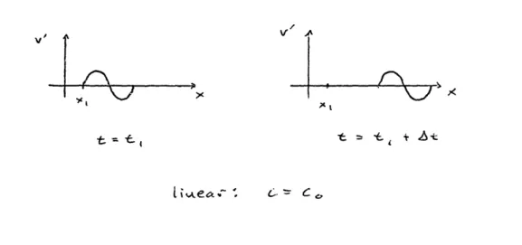
Fig. 1-1 Linear versus nonlinear waves. In the absence of dissipation, the linear wave never changes shape (except in an amplitude scale due to geometric spreading), while nonlinear waves always change shape as they travel.

V A'4

t -

, i+

.-t

Chapter 1 Introduction

character of a nonlinear acoustic wave is both a property of the material in which the wave propagates, as well as a result of the convective parts of the nonlinear wave equation. Schematic illustrations for linear waves which don't change shape, and nonlinear waves which do change shape, are shown in Fig. 1-1.

The introduction of acoustic dissipation also causes the wave shape to change in both the linear and nonlinear acoustic cases; that is why the dissipation-free case was used to mark the distinction between linear and nonlinear acoustic waves.

1.2 Prior Work in Nonlinear Acoustics

The nonlinear acoustics literature, up to the late 1950s and early 1960s, is quite sparse. The classic papers written on the subject range from the 1755 work of Euler up to the 1930's work by Fay and Fubini. Blackstock (1969) wrote a very complete review of the antique work in nonlinear acoustics from this period. I will not review the material among the papers described by Blackstock; rather, I refer the interested reader to his excellent paper and to the related paper that was an outgrowth of Blackstock's Ph.D. thesis (Blackstock, 1962). Though seldom mentioned in the literature, the mathematics considered and computationally used to model the focused explosive detonator for an atomic bomb, would have required substantial knowledge and understanding of many of the nonlinear acoustic principles brought to light much later on. It is entirely possible that considerable knowledge in nonlinear acoustics emerged from the Manhattan Project of World War II, especially considering the work by Bethe and Teller (1941), but only declassification of these documents will reveal the state of knowledge at the time.

Since the 1950s and 1960s, however, the field has expanded considerably, and the published literature in nonlinear acoustics since then is vast. The biannual meetings of the Acoustical Society of America have regular sessions devoted to various aspects of nonlinear acoustics. In addition, every two years or so, the International Symposium on Nonlinear Acoustics, or the ISNA

Chapter I Introduction

meetingl, is usually held at, or near, a center for nonlinear acoustics

research.

1.2.1 Prior Work in Nonlinear Acoustics at MIT

A number of papers in nonlinear acoustics have been produced at MIT, the first being a landmark paper by Professor R.D. Fay of the Electrical Engineering Dept. in 1931. Fay was later affiliated with the Underwater Acoustics Lab. of MIT during World War II. Fay renewed his interest in nonlinear and finite wave propagation in papers from 1956 and 1962. During the middle 1950s, K. Uno Ingard and his student D.C. Pridmore-Brown of the Physics Department studied the interaction and scattering of sound by sound (1955). This work was considered controversial; as recently as 1990, some of their results were still debated 2. L. Wallace Dean III (1962), from the Physics

Dept. and the Research Laboratory of Electronics, studied the interactions between sound waves. Dean also theoretically examined the problem Ingard had studied, for both beam-beam intersection, and beam-beam intersection in the presence of a hard object.

Two graduate students in the MIT Physics Department, L.N. Litzenberger (S.M. 1969, Ph.D. 1971) and L.P. Mix (Ph.D., 1971), studied linear and nonlinear ion acoustic waves within ionized plasmas and within magnetic fields, both students being directed by Prof. G. Bekefi. Ion acoustic waves are, in the words of Litzenberger, "... quite similar to ordinary sound waves in neutral gases except that long-range Coulomb interactions between charged particles rather than short-range collision forces between molecules dominate the

phenomenon."

S.W. Zavadil, an Ocean Engineering graduate student (O.E., 1976), created a computer code to model the nonlinear distortion of sinusoidal waves in viscous fluids, but he did not include relaxation nor heat conduction terms in the model, and his model was only valid for weak nonlinear waves; i.e. it would not handle shocks. He compared his model to that of Keck and Beyer (1960), and the agreement was very good.

Chapter 1 Introduction

Professor P.P. Lele of the Mechanical Engineering Dept, established a Laboratory for Medical Ultrasonics and Cancer Hyperthermia Center, and guided many graduate students throughout the last three decades. A number of the experiments done in the ultrasound/hyperthermia lab were related to nonlinear effects, principally including those by N. Senapati (1973) on cavitation and R. Handler (1976) on nonlinear sound absorption. Part of Handler's thesis was a section that estimated the harmonic generation for a focused sound beam using a model based on the work by Cook (1962). Handler was looking for an explanation for acoustically-induced thermal tissue damage. Handler concluded that the harmonic generation was an insufficient mechanism but cavitation might be sufficient.

J.A. Halsema's thesis (1992) and experiments, as mentioned at the beginning of this chapter, are both the most recent and apparently the first MIT-based foray into parametric sonar. Halsema used a .30-meter diameter piston transducer to radiate pulsed sound waves at roughly two frequencies: 184 kHz cw and a noise-like waveform in the range 169- to 179-kHz. By driving each of these frequency bands at large amplitude, he achieved nonlinear mixing of the two waves in the water, and created a difference frequency wave ranging from 5 to 15 kHz. These experiments were primarily performed in Boston Harbor, from the U.S.S. Constitution pier in Charlestown MA.

1.2.2 The State-of-the-Art in Nonlinear Acoustics

The state-of-the-art in nonlinear acoustics continues to unfold. As previously noted, every two or three years there is an International Symposium on Nonlinear Acoustics; the two most recent were hosted by the University of Texas, Austin (USA) in 1990 and the University of Bergen, Bergen (Norway) in 1593. The University of Texas/Applied Research Laboratory group in Austin, and the University of Bergen are recognized throughout the world as two of the principal research centers in nonlinear acoustics. In addition, nonlinear acoustics is playing a more important role in the use of ultrasound in medicine for therapeutic and diagnostic purposes, and it is intricately linked with the study of cavitation and sonoluminesence.

Chapter 1 Introduction

Today, there are principally four different approaches to the solution of nonlinear acoustics problems. The first, the oldest and most obvious, is the experimental approach. The second is the so-called phenomenological

approach (in this thesis, I instead use the term wave packet approach, or WPA). The third is based on the use of Burgers' equation (Burgers, 1939) which Blackstock (1964) fully covers. Trivett and Van Buren (1981) created a computational model based on Burgers' equation that used Fourier decomposition to solve the propagation problem entirely in the frequency domain. They compared the results for a single frequency 300 Hz cw plane wave example with a phenomenologically-based computer model by Van Buren (1975) for the spectral level of the fundamental and a number of the harmonics, and the agreement was superb. Their model was limited, however, to a single cw waveform input, and not to a plurality of pulsed waves at different frequencies. Both models, Trivett and Van Buren (1981) and Van Buren (1975) used an(,n) = al(wl)n 2 where n=2,3, ... etc. and a is the absorption coefficient for the fundamental frequency, to account for frequency-dependent absorption. This model accounts for sensible dissipation due to viscosity and heat conduction (in fresh water e.g.), but it does not account for relaxation absorption (in sea water or in air e.g.).

The fourth approach involves developing the wave equation in a parabolic form, and obtaining numerical solutions thereafter. This is the most popular computational method of record today, and is often the starting point for many papers authored by researchers at UTexas, Bergen and in the former Soviet Union (FUSSR). Presently there are at least two variants: one is a frequency-domain based method having origins in the FUSSR, and lately referred to as the KZK equation, initialed after the key theorists (Khokhlov, Zabolotskaya and Kuznetsov) who studied the problem during the late 1960s and early 1970s (see Zabolotskaya and Khokhlov, 1969; and Kuznetsov, 1971). The books by Beyer (1975), Rudenko and Soluyan (1977), and Novikov et al. (1987) each have sections which describe the mathematical development leading to the present form of the KZK equation. The other variant is the dissipationless Nonlinear Parabolic Equation, or NPE, of McDonald and Kuperman (1987) which is more amenable to time domain solutions. The NPE has the ability to model wave

Chapter I Introduction

propagation in the ocean in the presence of a sea surface, a seabed, and within a refracting water column. Thus it is useful for evaluation of broad propagation effects of linear and nonlinear waves as they are influenced by oceanic range- and depth-dependent features. What the NPE presently lacks, however, is a good absorption model. The NPE code includes an absorptive layer near the edges of the computational boundary to circumvent any numerical difficulties, but it does not include absorption (other than by weak shock theory, once shocks form) within the ocean waveguide itself3. This contrasts the statement made by Too and Ginsberg (1992)4 , who claimed the NPE uses dissipation both for numerical purposes, as well as for ordinary sound attenuation. The only attenuation included in the present form of the McDonald and Kuperman NPE for propagation is due to weak shock theory. The separate work by Too and Ginsberg, an adaptation of the NPE code for special purposes such as the near field study of nonlinear sound radiation from sound sources, included a first-order approximate dissipation term.

A brief summary of other techniques used in solving nonlinear acoustics problems appears in Physical Ultrasonics by Beyer and Letcher (1969), including: Fubini's method (1935); the perturbation analysis for the viscous case; the analytical methods of Fay (1931), Mendousse (1953), and Rudnick (1958); hybrid analytical-numerical methods by Fox and Wallace (1954), and Cook (1962); the use of Burgers' equation, particularly on a method by Blackstock (1964); and finally on Blackstock's (1966) bridging of the separate-region solutions of Fubini and Fay. One further attack on the problem of nonlinear acoustics was by Stepanishen and Koenigs (1987), where they used a time-dependent Green's function approach. They were able to obtain a closed-form expression for the radiated field which was proportional to the second spatial derivative of the square of the pressure envelope, in agreement with a result obtained by Berktay in the 1960's, but they needed to assume that the absorption was restricted to that of the primary wave in the pulse. Hence, it was a clever attack on the problem, it was useful for trendwise calculation of the radiated field both on- and off-axis, but it was not very useful for real problems.

Chapter 1 Introduction

1.3 Technical Approach

The technical approach used in this work is a form of the phenomenological

approach, a term borrowed from the work of Pestorius (1973), in modeling a sound wave which I refer to as a Wave Packet Approach (WPA). I refer to it as a Wave Packet Approach because it acts on small pieces of a wave pulse, wave packets, separately. This approach allows a locally valid wave equation to be

applied that includes absorption and nonlinear effects. I regard the term phenomenological approach somewhat cumbersome, not only because it is hard to say, but also because semantically it suggests the model is based strictly on a physical phenomenon rather than being grounded in mathematics. Related methods by Fox and Wallace (1954), Cook (1962), Pestorius (1973), Van Buren and Breazeale (1968a, 1968b), Van Buren (1975), and Handler (1976) all lacked a number of features which are included here. These features are a space/time-domain dissipation and a formal justification for using the phenomenological approach to show that it really does correctly model acoustic wave propagation from a theoretical basis. The WPA, by its use of space/time domain dissipation, allows wave propagation before, during, and after the shock-formed region, and in principle it does so without the use of weak shock theory. The fundamental reason for the presence or absence of weak shock theory in a computational model, and the consequent advantages and disadvantages, will be fully described in a section at the end of Chapter 5. A few of these key works are now described. Fox and Wallace (1954) used a graphical analysis, sans computer, as the starting point for their work. For a one-dimensional dissipationless medium, and starting with a pure tone sound wave, they divided the distance-to-shock into ten equal steps and proceeded to partially calculate the harmonic content (primary, plus first and second harmonics) of the wave, as it propagated from one step to the next. This allowed them to derive a growth factor for each harmonic, at each of the ten steps. An appropriate equivalent absorption factor (proportional to 2) was then introduced for each harmonic, at each step. The authors compared their model to experimental measurements made in water and in carbon tetrachloride, and the agreement was very good.

Chapter 1 Introduction

Cook (1962) used a similar procedure to that of Fox and Wallace, but used the Bessel-Fubini solution as the starting point, and did the modeling on a "high-speed computer." Blackstock has reviewed and showed the connection between the Fubini solution (before shock), and the solution of Fay's (saturated shock). Cook limited the numerical calculation to as many as 16 harmonics, assumed an 2 absorption dependence, and limited the propagation distance to 1/20-th of the shock formation distance. This sharply contrasted with the work of Fox and Wallace, who included only three harmonic terms, but made their calculations all the way to the dissipationless shock formation distance. Van Buren (1975) and Handler (1976) both used an approach based on the work by Cook.

Pestorius (1973) used the phenomenological approach as a basis for modeling high intensity noise-like waves propagating inside an air-filled tube, and he applied weak shock theory to account for the extinction of small wave perturbations by higher amplitude ones. A small dispersive component was added to the model to simulate the frictional interaction of the tube wall boundary with the pulse; this gave an absorption coefficient proportional to Vw, and also added a considerable dispersive feature. He then compared his computational results with those from in-air pulse tube experimental data, and

the agreement was very good, but it did slightly underestimate the absorption. An extension of Pestorius' work by Webster and Blackstock (1977) modeled the saturation of plane waves in air. Part of the work showed a comparison between experimental wave trace data and computed wave traces using the Pestorius algorithm.

1.4 A Brief on the Wave Packet Approach (WPA)

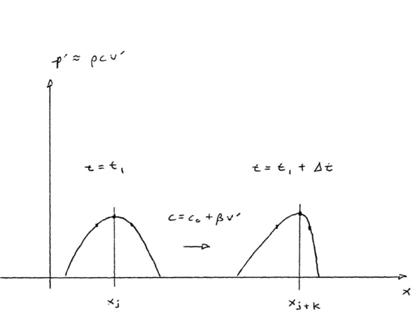
Starting with an initial acoustic wave pulse modeled at discrete x-node locations ... xj-l, xj, Xj+l, ... wave propagation is realized by mapping the acoustic pressure from a node location xj to a new node location Xj+k, as shown in Fig. 1-2. Hence, each small segment of the wave, herein called a wave

packet, moves to the j+k location on x at a speed c + /v' (this relation will be derived on the basis of a wave equation in Chapter 2), where v' is the acoustic

Chapter I Introduction

-I'"

ec

fi 1k

Fig. 1-2 Phenomenological Approach. In this approach, the wave is discretized by points, xj, and each point moves on the x-axis at a different propagation phase speed determined by cj = c + vj, where vj is the local acoustic particle velocity, is a constant related to the nonlinearity, and c is the sound speed for linear acoustics. In linear acoustics, all points xj travel at co.

Chapter I Introduction

particle velocity, and where k is the nodal step size (usually k >> j) which is equivalent to the distance traveled along x by the wave during a certain time interval. This wave model assumes forward propagation only, as in a one-way parabolic equation. This type of propagation algorithm is common to those previously used by Fox and Wallace (1954), Cook (1962), and others since.

The missing items from Pestorius' work were: a justification for using the phenomenological approach (via a wave equation); sound wave absorption that included viscous, relaxation, and heat conduction losses (Pestorius used a dissipation term that was valid for wall friction, but he intentionally did not include the losses for the propagating wave outside the wall boundary layer of the tube walls; hence his algorithm is incomplete for modeling unbounded waves in planar, cylindrical, or spherical propagation); and a general discussion for why weak shock theory was able to qualitatively represent the behavior of noise-like shock wave propagation modeled without the ever-present unbounded dissipation mechanisms of viscosity, heat conduction and

relaxation.

Other earlier uses of the phenomenological approach by Fox and Wallace (1954) and by Cook (1962) also lacked a rigorous wave equation justification. I originally planned to simply apply the phenomenological approach without worrying about whether it satisfied wave propagation notions including: conservation of mass, momentum, and energy (in the same manner as previous investigators). But as I progressed further, I decided that the lack of a formal justification would provide fertile ground for an officious professor attending the oral defense to ask a simple, yet hard-to-answer question. So I attempt to answer this question herein, and thus accomplish two things: to provide the justification absent from all previous phenomenological approaches, and to shortstop the question from being asked at my defense, by tackling it here.

The main distinction between the phenomenological approach used by others, and my so-called wave packet approach (WPA) is that space/time domain absorption, of the three significant dissipation types, is included. This contrasts with other means of solving the nonlinear wave equation by

Chapter 1 introduction

integro-differential methods, finite differences, or finite elements. These methods usually lump the dissipation into a thermoviscous term that is really only valid at a single frequency (often, the fundamental frequency in the problem under scrutiny). The precise details of the WPA used will be detailed in Chapter 4, after a case has been made for the nonlinear wave equation in Chapter 2, and after the dissipation terms for viscosity, relaxation and heat conduction have been derived in Chapter 3. These are the tools required before the WPA can be formally described.

1.5 Contributions Made by this Thesis

This thesis makes four significant contributions to the body of knowledge in nonlinear acoustics. The first is a computer-based time domain model for both linear and nonlinear acoustic waves. The central component in the code is a local nonlinear wave equation. This equation, written as a modification of the linear wave equation, provides the formal justification for using a wave packet approach (WPA).

The second major contribution is the formal development of time-domnain expressions for viscous, relaxation, and heat-conduction sound absorption coefficients. These expressions collapse into near-exact agreement with those in the existing literature under the special circumstance of pure tones. In the case of a sine wave exhibiting cumulative distortion, it can be clearly shown that the absorption at any point along the wave is uniquely related to the wave curvature in either p'-x (space) or p'-t (time) format. Hence, this theory provides a neat way to describe the absorption of a sound wave having arbitrarily complex shape, and provides a useful alternative to Fourier analysis as a means of explaining acoustic absorption. The computational model is sufficiently general to cover propagation in air, fresh water, sea water, glycerine, or a tissue/rubber model having a relaxation-dominated n

dependence.

The third major contribution is the investigation of the intersection and interaction of sound beams as a means of increasing thermal deposition in the sound-sound intersection region. This work was carried out in two ways: one

Chapter I Introduction

by laboratory experiments, and second by the use of the aforementioned computer code.

The fourth major contribution is an extention to the topic of shock theory, a special case of nonlinear acoustics. Traditional ways of approaching the development of weak shocks (where v' < c) have used the so-called equal-area rule to circumvent multi-valued solutions. This approach traditionally arrives from a dissipationless propagation model. When the shock occurs, and the wave becomes mathematically multivalued, the equal-area rule is imposed, whereby the multivalued part of the wave self-quenches. Hence, even though there was no dissipation used in the model, the equal-area rule provides attenuation even though it is unphysically realized. The mathematical development to attain the equal-area rule comes from conservation of certain sensible quantities (mass, momentum and energy), but nowhere are the ordinary attenuation means considered. The approach taken in this thesis retains all of the usual attenuation mechanisms completely up to the point where the wave would otherwise become multivalued. The key feature herein is that the attenuation mechanisms provide adequate means to prevent the

wave shape from becoming multivalued. The summary that can then be made is if no absorption is included in the propagation model, weak shock theory does a reasonable job of approximating the wave shape behavior and absorption at the shock. When absorption is correctly included in the propagation model, the strong second-order spatial gradient (from viscosity, relaxation, and heat conduction) at the shock location provides a doublet-like absorption function which attacks only the energy at the shock, and the need for weak shock theory disappears. There is, however, a strong reason related to computational time and resources, for simultaneously using both the space/time-domain absorption theory developed here and the equal-area rule. Other contributions in this thesis are comparatively minor in relation to the four mentioned above. They apply to the specific application examples shown later in Chapter 5.

Chapter I Introduction

1.6 Thesis Organization

This thesis is divided into six major parts beginning with Chapter 1, the Introduction, the one you have just read. Certain citations, listed at the end of the each chapter, include the author(s) name(s), year, and specific information such as page numbers or comments. The full citation, including paper or book title, is then included in the Bibliography at the end of the thesis.

The notion of the nonlinear and linear wave equations are derived in Chapter 2, as a means of formally justifying both he phenomenological and WPA approaches to wave propagation. Chapter 3 handles the three principal absorption mechanisms intrinsic to waves in fluids: viscosity, relaxation, and heat conduction. In Chapter 3 there is an occasional interchange of the terms

time-domain and spatial-domain. The main reason for the use of time-domain is to make the absorption used here distinct from the usual frequency-domain absorption universally used elsewhere. Absorption in a time-domain sense happens to be implemented here in a spatial-domain only because I use an label for the propagation axis rather than a time axis, and the choice of the x-labeling scheme is purely due to my preference for think of waves propagating in space rather than in time. Chapter 4 combines the ideas in Chapters 2 and 3 into a sensible computer model, and creates the WPA as a combination of the phenomenological approach and space/time absorption. Chapter 5 presents the reader with the most practical consequences of this thesis, and the most fun, because it covers a wide range of nonlinear propagation problems. Some of these problems, where experimental comparison is available, provide a degree of confirmation that the model is

correct.

Chapter 6 wraps up the thesis with discussion, conclusions, and some suggestions for future work. Several Appendices are included, followed by a full Bibliography for all the citations used in each chapter.

1see ISNA in the bibliography, various years.

2_{Westervelt, P.J. (1990). See this paper in Frontiers of Nonlinear Acoustics,}

Chapter I Introduction

3In the NPE User's Manual, from the subroutine damper: "there is no damping incorporated in the ocean itself nor is any icorporated in the sedimentary bottom; that is, no damping is incorporated from the 'nsurface' at the ocean surface down to the 'nsedbot', the bottom of the sediment."

4_{From the paper by Too and Ginsberg: "McDonald and Kuperman introduced a}

linear damping term in NPE for two reasons. Damping is needed to account for dissipation due to viscosity, heat transfer, and relaxation. In addition, it was intended to prevent the reflection of sound waves from the bottom of the simulation grid." See Too and Ginsberg (1992), p. 60, for this quote and for the first-order dissipation term.

Chapter 2 Nonlinear and Linear Acoustics

Chapter 2

Nonlinear and Linear Acoustics

This chapter discusses the notions of nonlinear and linear acoustics. The development of each is a spinoff of the combined equations of mass, momentum, and state for a fluid in a small control volume. When these equations are combined, a wave equation results. A first-order term approximation results in the linear wave equation, while the retention of first- and second-order terms results in a nonlinear wave equation. The development of a nonlinear wave equation into one that reduces to a linear wave equation provides a justification for using the wave packet approach (WPA) in solving nonlinear acoustic wave propagation problems.

2.1 Introduction

One of the goals in this chapter is a mathematical justification of a WPA for nonlinear acoustic propagation. In the related work of Fox and Wallace (1954), Cook (1962), and Pestorious (1973), no attempt was made at a mathematical justification for using the approach beyond pointing to the excellent agreement with experiments, a realistically powerful but somewhat incomplete defense. I give explicit reasons for the agreement here, by reconciling the WPA with a nonlinear wave equation.

Chapter 2 _{Nonlinear and Linear Acoustics}

evA~.,

Nj

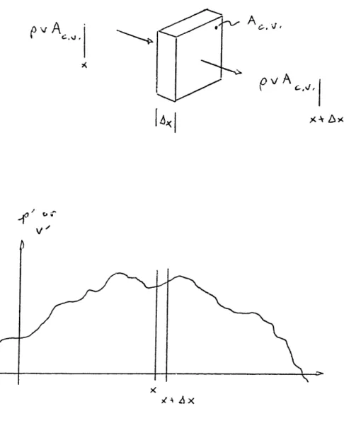
Fig. 2-1 Eulerian mass conservation.

AC,, I Adr Lx VI,

\

-·--I;

Chapter 2 Nonlinear and Linear Acoustics

Three principal characteristics are needed to justify the use of a WPA for nonlinear acoustics:

* first, when the wave amplitudes are small, linear acoustic waves are produced which don't change shape as they propagate. Thus a linear wave equation must be satisfied;

* second, that when the wave amplitudes are not small, the wave will change shape, or distort, as it propagates;

* third, that when a compression part of a wave advances in proximity with an adjacent rarefaction, a shock front is formed, which travels with roughly the average propagation speed of the compression and rarefaction fronts.

Since these three characteristics have been observed experimentally in real gases and liquids, they are regarded by all as. the truth. The WPA will produce the first phenomenon as long as losses are included, and the second phenomenon with or without the inclusion of losses. Both of these features require the use of a nonlinear acoustic wave equation, which is one of the goals in this chapter. Weak shock theory, applied as a special case of the WPA, provides an excellent model of the third phenomenon; however, the detail as to why the weak shock method works is lacking. Providing the answers to the why questions is one of the basic premises in this thesis, leading to more insight into nonlinear acoustic phenomena.

2.2

Mass Balance

Consider the Eulerian control volume shown in Fig. 2-1. The fluid control volume has thickness Ax and cross section area A v, where A v. is perpendicular to the vector v'. The limits on the thickness Ax are that it be much smaller than any acoustic wavelength taking passage, but much larger than the molecular mean-free-path. The first limit presents no problem for an analysis such as follows here, while the second limit is a sensible one,

Chapter 2 Nonlinear and Linear Acoustics

imposed by the entire notion of using a continuum-mechanics control volume

approach.

To keep both the algebra and the corresponding mathematical bookkeeping manageable, the analysis is limited to one-dimension (-D) along the x-axis. In many other acoustics and fluids works, the 1-D analysis gives the important features in relatively few pages. I do likewise here.

The important variables for this analysis are the pressure p, density p, and the particle velocity v. The variables p, p, and v are total quantities, and are respectively related to the acoustic quantities by the following relations:

total = ambient + acoustic

P = Po + p' , (2.1a)

p = Po + p' , (2.1b)

v = vo + v' . (2.lc)

The ambient variables are assumed constant, and henceforth in this thesis the ambient flow v will be assumed zero.

Returning to the control volume (C.V.) shown in Fig. 2-1, the aim is to balance the mass. The mass flux passing through the C.V. is pvAC v, which may then be separately evaluated on two sides of the C.V., once at x and again at x + Ax. The difference of the mass flux on each C.V. side (by subtraction) must equal the time rate-of-change of the mass enclosed inside the C.V. Formally, this is

pvAc.v.lx - pvAcv.l+ =

(pAAt

Rearranging Eq. (2.2), and using the fundamental theorem of calculus for partial derivatives, the result is

pvx + Vpx + Pt = 0, (2.3)

where x and t subscripted variables are a notation convention for partial derivatives. Note that

Chapter 2 Nonlinear and Linear Acoustics

where the material derivative

D/Dt /at + v.V

Eq. (2.3) is a nonlinear equation for mass conservation. To make it more useful, the full variables for density p and velocity v may be expanded into their ambient (with subscript "o") and acoustic quantities (with prime ' ) via Eqs. (2.1 a-c):

(po+ P')vx + v'Px + Pt = 0 . (2.4)

To linearize Eq. (2.4), only the first-order acoustic quantities are retained because the assumption is made that products of two or more acoustic quantities (resulting in second-order or larger-order terms) give values that are numerically trivial as compared to the first-order terms. The result is

povx + Pt = 0 . (2.5)

Note that each of the two terms in Eq. (2.5) has only a single primed (acoustic) variable, and so it is called a first-order mass conservation equation.

2.3

Momentum Balance

The same type of approach used to balance the mass in the C.V. is used to balance the momentum. Fig. 2-2 shows the same C.V. as in Fig. 2-1 with momentum now under consideration. We consider the time rate-of-change of the momentum in the C.V., so we need not only the forces acting on the C.V. at its left and right surfaces, but also the momentum flux quantity (pv).v. On each side, at x and at x + Ax, these are respectively

pAC.v. + pv2A.v. ;

pAc.v. is obviously force (pressure.area), and pv2Ae.v. is the force flux due to the particles at speed v crossing into (or out of) the C.V. By the same type of procedure previously used for the mass, the difference of the forces on the sides of the C.V. must equal the time rate-of-change of the momentum inside

Nonlinear and Linear Acoustics

5

X I

X t AX

Fig. 2-2 Eulerian momentum conservation.

I

A, :-.

l A,,,

']

Chapter 2 Nonlinear and Linear Acoustics

the C.V., or:

(pA,.v. + pv2Ac.v.)lx - (pAc.v. + pV2Ac.v.)[x+Ax - at (PAc Ax v), (2.6)

where the fluid is assumed lossless and irrotational. Rewritten in subscripted partial derivative form, Eq. (2.6) becomes

(pv)t + (pv2)x + Px = 0 . (2.7) Expanding Eq. (2.7) into component terms yields:

pvt + pv.vx + v (pt + (PV)x} + Px = 0 . (2.8) Eq. (2.8) is immediately simplified by recognizing that Eq. (2.4) makes the bracketed term, (Pt + (pv)x), equal to zero. Hence Eq. (2.8) becomes

pvt + pv-Vx + Px = 0 . (2.9)

The density and particle velocity are then expanded into ambient plus acoustic

variables:

- P = (Po + )vt + (Po+ p')v'V . (2.10) Eq. (2.10) is a nonlinear momentum equation having first-, second- and third-order terms. The first-order approximation is the linear momentum equation given by

-Px = Povt . (2.11)

2.4

Equation of State: a Pressure-Density Relation

The mathematical relations for pressure-density (p-p) may be written in terms of a Taylor series expansion. Most authors1 use series expansions of p(p), rather 2 _{than series expansions of p(p). It will be more convenient (later) to}

use the former approach, hence for now we write

= +

A

Chapter 2 Nonlinear and Linear Acoustics

where A poc2, and the condensation s p/po. Then by rearranging Eq. (2.12), and substituting Eq. (2.1a)

p = P- = poc2 [s + 2A S2 + -- s3 + O(s4 )] . (2.13)

2A 6A

In the event that s2, and higher-order terms in s, are considered small compared to the first-order term s, then we have a linear equation of state

p' = poc 2 s = c2 p' . (2.14)

2.5

The Wave Equation:

Linear & Nonlinear Forms

Now that we have the basic mass, momentum, and state equations to work with, wave equations may now be developed for both linear acoustics, and for nonlinear acoustics.

Linear Acoustic Wave Equation

The linear acoustic wave equation is derived from the linear equations of mass, momentum and state; these are respectively Eqs. (2.5), (2.11) and (2.14). The usual procedure is to take dt on the mass equation (2.5), take dldx on the momentum equation (2.11), and add the results. This eliminates the cross partial derivative d2/(dtdx) terms. Then the acoustic density p' is eliminated by substitution of the equation of state, Eq. (2.14), so that the entire equation is in terms of the acoustic pressure p'. The result is

a2p' = I a2p, (2.15)

ax2 c2 at2

Other manipulations are possible to write the wave equation in terms of p' or v' (see Jensen et al., 1994), where each variable merely substitutes for p' in Eq. (2.15). Eq. (2.15) is in the general form of a standard 1-D linear wave equation which admits arbitrary solutions f(x+cot) and g(x-cot). Note that the shape of the wave never changes as the wave travels, and that every point and every

Chapter 2 Nonlinear and Linear Acoustics

portion along the wave travels at the same speed c, independent of the pressure amplitude of the wave.

Nonlinear Acoustic Wave Equation

The procedure for deriving the nonlinear wave equation is the same as the linear case, but there are many more terms to deal with. What follows is considerable algebra, but it is shown here for completeness as it is seldom written out fully. Starting with the nonlinear mass equation, Eq. (2.4), take

d/dt, with the result

- Ptt = PoVtx + PxVt + p'Vtx + Ptvx + V'Ptx · (2.16)

Then take dldx on the nonlinear momentum equation (2.10), with the result Pxx = - povt - Pxvt - p'vxt - (Po + p')(vx)2 - (po + p')v'vxx - pxv'vx . (2.17)

Adding Eqs. (2.16) and (2.17) eliminates the underlined terms in each equation. The result is

Ptt = Pxx + (Po + P')(Vx)2 + (o + p')v'vxx + px'v - - 'tVx . (2.18)

Eq. (2.18) appears formidable, but there are a few modifications that may be made to make it more closely resemble a familiar wave equation. First, we need to rewrite the entire equation singularly in terms of p', or p'. Because of the way the equations have been developed thus far, it will be easier to eliminate

p'. This is done by using the last of the three equations, the equation of state (2.13) which is repeated here,

p' = pc2 [+ s + B +

+(s

2A 6A

Chapter 2 Nonlinear and Linear Acoustics

spatial derivative on the equation of state. The result is

Pxx = co2 { xx + B [() 2 xx + C [ 2p(p) 2 + (p) 2 Pxx]

A po 2A 2

+ 0(s

_).

_(2.19)

In Eq. (2.19) we see that there are three Pxx terms; rewriting Eq. (2.19) with these terms grouped together we have

Pxx pxx c2 { + A (-). + -C ()2 + 2 {

.

Po AO + 2A Co Apo Ap 2

+ O0s4}. (2.20)

Eq. (2.20) was written by combining Eq. (2.13) with the impedance relation:

p' = poc 2 Is + B s2 + -Cs3 + O(s4)] = pocoV',

p = p 0 [+2A 6A

and by noting that

Po

V

~ 1Co

~

+

vo

(2.21)

po Co [1+ Bs+ + Cs2+( s O(3)] C

2A 6A

Now that we have what we want (Pxx) from the equation of state, we can substitute Eq. (2.20) into Eq. (2.18), thus eliminating the acoustic pressure variable p' as we had intended:

X1B

+

(vo'

(v')

2...}

+ c

B (px)

+ C p()2

A pxo 2 A Co A po A p

+ po(v)2 +

p'(v;)

.... 2

--.-

-...

8---One assumption made in writing Eq. (2.22) is that the O (s4 ) term, a fourth-order product of acoustic variables, has been omitted due to smallness. Eq. (2.22) may be further simplified by additional assumptions, so we must deal with the

Chapter 2 Nonlinear and Linear Acoustics

overlined and underlined terms which are all second- and third-order products of acoustic variables. The first term, labeled 1, can be discarded because the accompanying term in the braces {--) is considerably larger. This is shown by rewriting the brace term as

B Po + CP P. } Px

The term inside the braces may be evaluated as follows. For either fresh or sea water, B/A is about 5, and C/A is about 35; hence if po >> 7p' then the (C/A)p' term may be discarded. For air, B/A is about 0.4 and C/A is about 0.24; hence if po >>

.63p' then the (C/A)p' term may be discarded. Because p >> p' even for a large amplitude sound in water or air, the (C/A)p' term is safely ignored3, so we can safely discard term 1 in Eq. (2.22).

Terms 3 and 5 in Eq. (2.22) are discarded not only because they are third-order products of acoustic variables, but because they are also much smaller than terms 2 and 4 respectively, again because p >> p'. Term 6 is discarded because it is a third-order product of acoustic variables, which we assume small compared with the first- and second-order terms. With terms 1, 3, 5, and 6 discarded, and discarding any other third-order products, we have

= Px c 1 + () + o2 B (px)2 v + p(vx) 2 + povvxx

A o A po

ptvx - v tx (2.23)

By using the relation given in Eq. (2.21), we can rewrite the derivatives of v' in Eq. (2.23) in the iurm of density p':

tt = Pxx 2 1 + AB (Y )+ 2 B (x) 2 + (c2/p)(p) 2

A Co APx P

2+

Pxxo

(

Chapter 2 Nonlinear and Linear Acoustics

or reorganized as

Ptt = Pxx c2 { 1 + + 1)

}

PO -PPx P(-o)PtX (2.24)

Eq. (2.24) is further rewritten to convert the time derivatives on the right side to spatial derivatives, by using the wave space-time duality convention that

a/at <---> -co . a/ax .

This makes the right side of Eq. (2.24) entirely populated either by Pxx terms, or by Px terms. Hence

Pt = Px c2 { 1 + + 2)(o) B )(px)2 . (2.25)

The double underlined term in Eq. (2.25) has entirely positive constants, and the single underlined term is both positive-valued and second-order due to the square exponent. We shall discard this term on the basis that it is second-order compared with the remaining effectively first-order terms.

More interesting however is the form of the rest of Eq. (2.25): it has the form of a linear wave equation if the brace term, i.e. { .... , is considered to be a

modification of c. Taking the brace term as a modification of c2, then the

non-underlined part of Eq. (2.25) is treated as a linear wave equation with first-order acoustic terms, and we discard the underlined terms which are fully second-order:

2

Ptt = Ceffective Pxx, (2.26)

where 2 ffective = c

{

Recalling that C = p from Eq. (2.21), we can compare the magnitude of the brace components in Eq. (2.27):

1: ( + 2)