HAL Id: tel-01712811
https://pastel.archives-ouvertes.fr/tel-01712811
Submitted on 19 Feb 2018
HAL is a multi-disciplinary open access
archive for the deposit and dissemination of
sci-entific research documents, whether they are
pub-lished or not. The documents may come from
teaching and research institutions in France or
abroad, or from public or private research centers.
L’archive ouverte pluridisciplinaire HAL, est
destinée au dépôt et à la diffusion de documents
scientifiques de niveau recherche, publiés ou non,
émanant des établissements d’enseignement et de
recherche français ou étrangers, des laboratoires
publics ou privés.
application to an emergency call center
Vianney Boeuf
To cite this version:
Vianney Boeuf. Dynamics of a two-level system with priorities and application to an emergency
call center. Optimization and Control [math.OC]. Université Paris Saclay (COmUE), 2017. English.
�NNT : 2017SACLX120�. �tel-01712811�
NNT : 2017SACLX120
THÈSE DE DOCTORAT
DE L’UNIVERSITÉ PARIS-SACLAY
préparée à
L’ÉCOLE POLYTECHNIQUE
ÉCOLE DOCTORALE N
o574
Mathématiques Hadamard (EDMH)
Spécialité de doctorat : Mathématiques
par
Vianney Bœuf
Dynamics of a two-level system with priorities and
application to an emergency call center.
Thèse présentée et soutenue à Palaiseau, le 18 décembre 2017
Composition du jury :
Xavier Allamigeon (Inria & CMAP, École polytechnique) Co-directeur de thèse
Thomas Bonald (Télécom ParisTech) Rapporteur
Stéphane Gaubert (Inria & CMAP, École polytechnique) Directeur de thèse
Alessandro Giua (Universités Aix-Marseille et Cagliari) Rapporteur
Pierre L’Ecuyer (Université de Montréal) Rapporteur
Jean-Jacques Loiseau (LS2N, université de Nantes) Président
Philippe Robert (INRIA de Paris) Examinateur
«Il n’y a que les routes qui sont belles... »
À mes parents. Pour l’esprit mathématique que vous m’avez légué ; pour mon goût mathématique que vous avez éveillé et fait s’épanouir. Cette thèse vous doit beaucoup.
Remerciements
Je tiens à remercier en premier lieu mon directeur de thèse Stéphane Gaubert et mon co-directeur Xavier Allamigeon. Merci à tous deux pour m’avoir conduit sur ces belles routes scientifiques, et pour m’avoir beaucoup transmis. Merci à Stéphane pour ta science encyclopé-dique et ton fidèle soutien. Merci pour m’avoir accueilli jusqu’à chez toi lorsqu’il fallait traiter des urgences. J’associe naturellement Marianne à ces remerciements. Merci à Xavier pour la qualité de nos échanges, ta rigueur et la touche informatique dont cette thèse a beaucoup profité. Merci à vous deux pour tous ces repas si sympathiques, et la richesses de vos conversations.
Merci à Thomas Bonald, Alessandro Giua et Pierre L’Ecuyer, d’avoir bien voulu être rap-porteurs de ma thèse. Merci pour leur lecture avisée de mon manuscrit. Je remercie aussi sincèrement l’ensemble des examinateurs d’avoir accepté, parfois en venant de très loin, de venir siéger à mon jury.
Cette thèse doit beaucoup à la Brigade des sapeurs-pompiers de Paris et à la Préfecture de police de Paris. Je remercie chaleureusement Stéphane Raclot, présent sur tous les sujets. Merci pour ton accueil à la Brigade. Merci pour ta capacité à interagir avec des scientifiques et à donner à tout cela un caractère opérationnel. Merci à Régis Reboul. Merci à tous les pompiers qui m’ont accueilli parmi eux, Frédéric Derreati, Pascal Dillenseger, David Vigier, Floriane Brill, Benjamin Fouilleul et l’ensemble de l’équipe SIOP et GGO. Merci au lieutenant-colonel Vilbé d’avoir particulièrement cherché à utiliser mon expertise (parfois sans doute surestimée !) avec une grande exigence, et pour votre soutien sur de nombreux sujets. Merci au BPO et notamment les lieutenants-colonels Deshayes et Cros. Merci aux capitaines Éric Faraon et Éric Gauyat. Merci à Philippe Boubel et François Botella. Merci à Carl de Barmon et Roman Lorencki. Merci aux médecins et aux juristes de la Brigade, avec qui j’ai toujours eu plaisir à échanger.
Mes remerciements s’étendent aux pompiers instructeurs qui m’ont formé aux premiers secours en équipe (et notamment le sergent-chef Lefèbvre), et aux pompiers du centre de secours de Montmartre qui m’ont accueilli pour des immersions en garde VSAV. Je salue aussi l’ensemble des camarades VSC de ma formation.
Les passages à l’équipe RAP ont toujours été des moments agréables et la personnalité et la disponibilité de Philippe Robert y sont pour beaucoup. Merci Philippe pour notre travail ensemble, merci pour m’avoir initié à la théorie de la mesure et à bien d’autres objets stochas-tiques, et pour les footings à 11h30 précises. Merci à Christine, Guilherme, Wen, Renaud, Sarah, Davit et les autres pour les agréables moments de détente, et pour ce séjour sympathique à Chicago.
Au CMAP, je veux remercier tout ceux à qui j’ai pu exposer des problèmes de mathéma-tiques, et j’espère n’oublier personne en citant Marianne Akian, Vincent Bansaye, Yacine Chi-tour, Hadrien De March, Carl Graham, Benjamin Heymann, Ludovic Sacchelli, et, plus encore, Erwan Le Pennec, qui m’a apporté de précieuses informations sur le langage R et sur certaines méthodes statistiques. Je remercie aussi l’équipe administrative du CMAP et de l’INRIA, no-tamment Nassera Naar, Alexandra Noiret, Jessica Gameiro et Corinne Petitot. J’y associe mes remerciements à Sylvain Ferrand.
Je remercie Frédéric Meunier pour mon super stage de recherche opérationnelle sur le train
shunting. Merci de m’avoir permis de croire que je pouvais non seulement chercher, mais aussi
trouver. Merci aussi pour le TD d’optimisation aux Ponts, que j’ai eu grand plaisir à donner. Merci à Sébastien Blandin. Merci à Olivier Klopfenstein pour le projet à l’ENSTA.
Je remercie les chercheurs de l’ANR Democrite et notamment Emmanuel Lapébie. Je re-mercie aussi les huit élèves polytechniciens qui ont travaillé au cours de ces trois années sur la PFAU ou sur des aspects liés.
J’ose à peine citer au CMAP tous ceux avec qui j’ai eu plaisir à échanger, à passer des repas ou des pauses cafés. Je pense en premier lieu à mes co-bureau Etienne, Antoine, Gustaw, Aleksey, Florine, Jean-Bernard, Céline, Pierre. Merci particulièrement à mon « prédécesseur » Antoine et mon « successeur » Jean-Bernard : cela crée des liens particuliers ! Je salue aussi Joon, Perle, Hadrien, Aline, Romain, Antoine, Nikolas, Mateusz et encore de nombreux autres !
Mes camarades des autres labos, Lucile, Simon et Olga, méritent aussi de grands remercie-ments. Merci beaucoup à Lucile pour l’escalade.
Merci, dans un autre registre, à Monsieur Christian Makhmoufi pour avoir retrouvé mes affaires de thèse au fond d’un ruisseau à Beauvoir-en-Royans après un vol à la roulotte.
L’amitié se mesure entre autres par la capacité à reprendre avec passion la conversation après un intervalle parfois prolongé par la distance géographique, le travail ou les responsabilités diverses. Je ne prendrais évidemment pas le risque de citer tous les amis avec qui j’ai pu passer du temps pendant ces trois années, mais qu’ils soient ici chaleureusement remerciés. Je dois une dédicace toute particulière à mes quatre « chapeaux verts », Axel, Gaétan, Gaëtan et Matthieu qui savent toute l’affection que je leur porte. Pour Axel s’ajoutent des remerciements pour nos nombreuses discussions scientifiques et d’avenir. Je remercie aussi ici les Oyens pour Oya, et les Cramés, Matthieu, Étienne, Guillaume, Alexandre, Augustin, Maximilien, pour près de deux ans de coloc dans un super esprit.
Merci à ma famille, qui représente tant pour moi, et est un vrai ressourcement. Merci à Céline, Mathilde, Solène, à Éric et à mes nièces et neveu. Merci pour ces liens inconditionnels qui nous unissent. Mes remerciements du fond du cœur vont à mes parents pour tout ce que vous m’avez transmis et donné, depuis les premiers jours et bien sûr pendant ces trois dernières années. Cette thèse vous est dédiée.
Merci à ma deuxième famille depuis peu, et à mes nouveaux beaux-frères et belles-sœurs. Merci particulièrement à Père et Mère, pour m’avoir offert des conditions de travail épatantes dans des lieux magnifiques.
J’adresse enfin mes remerciements aux deux personnes qui comptent le plus dans ma vie : merci Sixtine d’avoir été un petit bébé si adorable et si sage pendant tes dix premiers mois. En plus de faire l’admiration de ton papa, tu as aussi grandement facilité l’avancement de ma thèse. Merci enfin, surtout, à mon épouse Isabelle. Merci pour tous tes sacrifices pendant la rédaction de ma thèse, tous ces jours de congés sans moi, ces soirées, ces weekends où tu devais, non seulement te passer de moi mais aussi t’occuper de Sixtine et de la maison. Cette fois-ci la thèse est bel et bien bouclée, quel soulagement ! Merci pour ton dévouement et ta sollicitude. Merci, plus fondamentalement, d’être une si belle raison d’être et d’aimer depuis plusieurs années.
v
Abstract
We analyze the dynamics of discrete event systems with synchronization and priorities, by means of Petri nets and queueing networks. We apply this to the performance evaluation of an emergency call center.
Our original motivation is practical. In 2016, a new emergency call center became operative in Paris area, handling emergency calls to police and firemen. The new or-ganization includes a two-level call treatment. A first level of operators answers calls, identifies urgent calls and handles (numerous) non-urgent calls. Second level operators are specialists (policemen or firemen) and handle emergency demands. In this archi-tecture, some calls are qualified as extremely urgent and receive a priority treatment. We are interested in the performance evaluation of bilevel systems corresponding to this general description.
We propose three different models addressing this kind of systems. The first two are timed Petri net models. We enrich the classical framework of free choice Petri nets by allowing conflict situations in which the routing is solved by priorities. The main difficulty in this situation is that the dynamics becomes non monotone.
In a first model, we consider discrete dynamics for this class of Petri nets. We prove that the counter variables of the Petri net are solutions of a piecewise linear system with delays. We investigate the stationary regimes of the dynamics, and characterize the affine ones as solutions of a piecewise linear system, which can be thought of as a system of rational equations over a tropical (min-plus) semifield of germs. Numerical experiments show that, however, convergence does not always holds towards these affine stationary regimes.
The second model is a infinitesimal version of the previous one. For the same class of Petri nets, we introduce a dynamics expressed by differential equations, so that the tokens and time events become continuous. For this differential system with discontinuous righthandside, we establish the existence and uniqueness of the solution. The benefit of this continuous model is that the discrete time pathologies disappear. We show however that the stationary regimes are the same as the stationary regimes of the discrete time dynamics. Numerical experiments tend to show that, in this setting, convergence effectively holds.
We also model the emergency call center described above as a queueing system, taking into account the randomness of the different call center variables. For this system, we prove that, under an appropriate scaling, the dynamics converges to a fluid limit which corresponds to the differential equations of our Petri net model. This provides support for the second model. Stochastic calculus for Poisson processes, generalized Skorokhod problems formulations and coupling arguments are the main tools used to establish this convergence.
Hence, our three models of an identical emergency call center yield the same schematic asymptotic behavior, expressed as a piecewise linear system of the parameters, and describing the different congestion phases of the system.
In a second part of this thesis, simulations are carried out and analyzed, taking into account the many details of our case study. The simulations confirm the schematic behavior described by our mathematical models. We also address the complex inter-actions coming from the heterogeneous nature of level 2.
Resumé
Nous analysons la dynamique de systèmes à événements discrets avec synchronisation et priorités, au moyen de réseaux de Petri et de réseaux de files d’attente. Nous appliquons cela à l’évaluation de performance d’un centre d’appels d’urgence. Notre motivation est en premier lieu pratique. En 2016, un nouveau centre d’appels d’urgence a été mis en place pour l’agglomération parisienne, traitant les appels pour la police et les pompiers. La nouvelle organisation comporte deux niveaux de traitement. Un premier niveau d’opérateurs répond aux appels, identifie les appels urgents et traite les appels non urgents. Les opérateurs de second niveau sont spécialistes (policiers ou pompiers) et traitent les demandes d’intervention. De plus, certains appels sont identifiés comme très urgents et bénéficient d’un traitement prioritaire. Nous nous intéressons à l’évaluation de performance de divers systèmes correspondant à cette description générale.
Nous proposons trois modélisations différentes. Les deux premières sont des modèles de réseaux de Petri temporisés. Nous enrichissons le cadre classique des réseaux de Petri à choix libres en autorisant des situations de conflit où le routage est résolu par des priorités. La principale difficulté est alors que l’opérateur de la dynamique n’est plus monotone.
Dans un premier modèle, nous proposons une dynamique discrète pour cette classe de réseaux de Petri. Nous prouvons que les variables compteurs du réseau sont les solutions d’un système affine par morceaux avec retards. Nous étudions les régimes stationnaires de cette dynamique, et caractérisons les régimes affines comme solutions d’un système affine par morceaux, qui peut être vu comme un système d’équations rationnelles sur le semi-corps de germes tropical (min plus). Les applications numé-riques montrent cependant que la convergence ne se fait pas toujours vers ces régimes stationnaires affines.
Le second modèle est une version infinitésimale du précédent. Pour la même classe de réseaux de Petri, nous proposons une dynamique sous forme d’équations diffé-rentielles : les jetons et le temps deviennent continus. Pour ce système différentiel discontinu, nous établissons l’existence et l’unicité de la solution. L’avantage de cette modélisation continue est que les pathologies du temps discret disparaissent. Nous montrons cependant que les régimes stationaires sont les mêmes que ceux de la dy-namique discrète. Les simulations numériques semblent montrer que la convergence s’obtient effectivement dans ce cas.
Nous modélisons aussi le centre d’appels d’urgence comme un réseau de files d’attente, prenant ainsi en compte le caractère aléatoire des différentes variables du centre d’ap-pel. Pour ce système, nous prouvons que la dynamique, après une transformation d’échelle, converge vers une limite fluide, qui correspond au système d’équations diffé-rentielles de notre modèle de réseau de Petri. Cela conforte notre seconde modélisation. Les principaux outils de la preuve de convergence sont le calcul stochastique pour les processus de Poisson, des formulations en terme de problème de Skorokhod généralisé, ou encore des arguments de couplage.
Ainsi, nos trois modèles d’un même centre d’appels d’urgence définissent un même comportement asymptotique schématique, exprimé comme un système linéaire affine par morceaux, décrivant différentes phases de congestion du centre.
Dans une seconde partie de cette thèse, nous analysons des simulations poussées, pre-nant en compte les nombreux détails de notre étude de cas. Les simulations confirment le comportement schématique prédit par nos modèles mathématiques. Nous discutons aussi des interactions complexes provenant de la nature hétérogène du niveau 2.
Contents
1 Introduction 1
1.1 Priority routing of calls in an emergency call center . . . 1
1.2 The “emergency physician” paradox . . . 3
1.3 Beyond non-expansive operators . . . 5
1.4 Contributions . . . 8
Part I
A Dynamical Analysis
11
2 Preliminaries on Petri nets 13 2.1 Untimed Petri nets . . . 142.2 Structural analysis of Petri nets . . . 19
2.3 Timed semantics of Petri nets . . . 23
2.4 Routing rules in Petri nets . . . 25
2.5 Three Petri net examples . . . 27
3 Discrete dynamics and fluid approximation for Petri nets with priorities 33 3.1 Introduction . . . 33
3.2 Piecewise linear dynamics . . . 35
3.3 Computing stationary regimes . . . 43
3.4 Application: the emergency call center PN . . . 46
3.5 Application: the SR Petri net . . . 48
3.6 Numerical experiments . . . 50
3.7 Concluding remarks . . . 53
4 Hybrid dynamics of Petri nets with priorities 55 4.1 Introduction . . . 55
4.2 Hybrid dynamics of Petri nets with time attached to places . . . 57
4.3 Well-posedness of the dynamics . . . 61
4.4 Stationary solutions . . . 67
4.5 Numerical experiments . . . 71
4.6 Concluding remarks . . . 73
4.7 Proof of Proposition4.6 . . . 73
5 A stochastic analysis of a network with two levels of service 77 5.1 Introduction . . . 77
5.2 The Stochastic Model . . . 81
5.3 Analysis of Auxiliary Processes . . . 84
5.4 Asymptotic Study of the Blocking Phenomenon . . . 91
5.5 Concluding remarks . . . 97
Part II
Case study: simulations and analysis of an emergency
call center
99
6 Case study: simulations and analysis of an emergency call center 101 6.1 Data analysis of an emergency call center . . . .1026.2 The impact of having separated groups of operators at level 2 . . . .105
6.3 Other lessons from simulations . . . .109
6.4 Concluding remarks . . . .112
6.5 A few words on our simulations . . . .113
Bibliography 114
Chapter
1
Introduction
1.1 Priority routing of calls in an emergency call center . . . 1
1.2 The “emergency physician” paradox . . . 3
1.3 Beyond non-expansive operators . . . 5
1.4 Contributions . . . 8
1.1
A practical motivation: priority routing of calls in an
emergency call center
The new organization of emergency call treatment in Paris area This thesis finds its source and impetus in a project led by Préfecture de police de Paris (PP)1, in collaboration with the Brigade de sapeurs de pompiers de Paris (BSPP)2.
Since early 2016, a new organization of the treatment of emergency calls became operative in Paris area. In a single call center, emergency calls to Police (17), Firemen (18)3and untyped emergency calls (112), are answered, and treated according to the type of emergency. The new architecture involves two levels of operators. At the first level, operators detect the type and urgency of the calls, handle (numerous) non urgent calls, and transfer urgent calls to second level operators, police or firemen. At the second level, operators handle the call request, and dispatch emergency means, if needed. The second level is split into two pools of operators, policemen and firemen. They have specific missions, and answer different types of calls. In contrast, the first level is common to police and firemen.
For the project leaders (see [dpdP16]), this new organization aims at improving emergency calls treatment, by identifying them faster and dedicating operators to them. Another objective is to decrease waiting times, by increasing the number of operators, and pooling part of police and firemen resources. Finally, gathering police and firemen operators in the same place is meant to bring a better coordination between both security forces for joint operations.
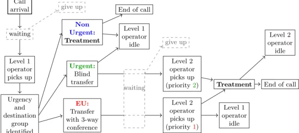
In order to improve the quality of the response for the most urgent calls, a key feature of the new organization is that, once they are identified as such, extremely urgent (EU) calls should always be in line with an operator. As a consequence, when a level 1 operator transfers a call, if the destination level is busy, the operator waits with the caller until a level 2 operator is available. Moreover, if several calls are waiting for the same destination level, EU calls have priority. We depict in Figure1.1the itinerary of an emergency call in the call center. Note that
1. Paris security authority 2. Paris Fire Brigade 3. also in charge of first aid
Call arrival waiting Level 1 operator picks up Urgency and destination group identified Non Urgent: Treatment Urgent: Blind transfer Level 1 operator idle End of call EU: Transfer with 3-way conference waiting Level 2 operator picks up (priority1) Level 1 operator idle
Treatment End of call Level 2 operator idle Level 2 operator picks up (priority2) give up give up
Figure 1.1 – Schematic flow chart of a call treatment in the two-level emergency call center.
this is a simplified model. For example, a few partner organizations have direct access to level 2 (e.g., gas or electricity companies, public transportation operations centers).
This two-level architecture, together with the blocking of level 1 operators when a group of level 2 is busy, does not enter in the classical call center models, nor in the standard queueing network models. Specifically, these models would fail to account for the fact that the capacity of level 1 is diminished when a level 2 group is saturated. Moreover, we shall also not expect an exactly solvable Markov model: in these complex configurations, the invariant distribution cannot have a simple analytical expression.
This calls for exploring mathematical models in more details, in order to provide suitable formulæ for this system. From a user point of view, one would like to compute performance bounds, performance indicators, depending on the parameters of the system, as well as to deliver a general understanding on the different regimes and limit behaviors. In such situations, simple operating principles are as helpful as complex simulation-based tables and charts. Furthermore, a flexible tool is required, as the detailed architecture may vary in time and depending on the successive analyses and feedbacks.
This is the kind of results we endeavored to deliver to the project leaders and heads of the new emergency call center.
Petri net modeling Petri nets are a modeling language appropriate to account for concur-rency and parallelism. A Petri net is a graph whose nodes are transitions and places, connected by directed arcs. Places hold tokens, which circulate from place to place, moved by transition
firings. A transition can fire only if a token is available in each of the upstream places, and
when a transition fires, it consumes (removes) one token in each upstream place, and produces (creates) one token in each downstream place. Therefore, a transition operates as a local syn-chronization and distribution module in a network. Tokens typically represent resources in a manufacturing process, or requests and servers in a communication network.
A Petri net modeling a simple call center is given in Figure1.2.
Petri nets can also be given a timed semantics, in which case the circulation of tokens can encounter delays, or traveling times. In our simple call center, for example, we associate with each place a holding time: a token entering a place can leave it (by the firing of a downstream transition) only after having sojourned a given delay in this place.
Being able to model complex concurrency phenomena, together with a timed interpretation, Petri net is an appropriate, workable tool for modeling our two-level emergency call center.
On top of its flexibility, it is also a very convenient language for interacting with practitioners. Petri net’s graphical representation, including token evolution by transition firings, makes it a directly intelligible language, and this facilitates the delicate process of modeling a real system.
Section 1.2 The “emergency physician” paradox 3 τe Waiting calls τi Idle operators τc Conversation
Call arrival Pick up Hang up
Figure 1.2 – Petri net of a simple call center. Transition are represented by thick black segments, and places by circles. Tokens are dark red dots in places. The arrival of calls is modeled by the left-most transition, and their release by the right-most transition. Here, there are two operators, both in conversation with a caller, and three other calls queueing. Ingreen, we have represented the places’ holding times∗.
∗Note that τ
edoes not represent a token waiting time, but rather a fixed delay before entering in the queue, for example, an automatic welcome message. The waiting time if no operator is idle comes in addition to this holding time.
Priority Among the characteristics of the system described above, the priority allocation of level 2 operators to EU calls is the only (but crucial) non standard Petri net feature. In this thesis, we formalize priority routing of tokens in a timed Petri net.
Previously, Petri nets with priorities had already been studied in a non timed setting, which involves order relations between all transitions in the net. See for example [BK92]. In contrast, the priority rules that we study in our timed setting are local, restricted to clusters (group of connected upstream places and output transitions), because it takes a certain amount of time for a token to go from a cluster to another.
We found our inspiration in the anterior work of Farhi, Goursat and Quadrat [FGQ11], where such local priority routings are applied to a timed road traffic model.
Specific features of an emergency call center Emergency call centers differ from classical call centers in terms of objectives and characteristics.
Firstly, serving all callers, and serving them with minimum waiting times, is a much more involving imperative in an emergency call center, for which spared minutes and answered calls result in direct benefits in terms of lives, health and goods.
Secondly, an emergency call center must be designed, not only to face every-day situations, but also critical situations arising from expected or unexpected events (e.g., storms, floods, terrorist attacks), in which the characteristics of demand (incoming calls) may be completely different. In such situations, one would like to design specific procedures to alert the people in charge, and to ensure that calls are served. This comprises resorting to reinforcements, and shifting in degraded modes.
In our work, we find simulations and formal analyses to be appropriate and complementary to account for such critical situations. While simulations allow one to focus on specific case studies, and to test in silico the performances of the planned organizations in the critical situations observed in the past, formal analyses provide information on the general behavior of the system, including at the limits. Besides, in our models, we will be particularly interested in stressed situations, in which the system is saturated in incoming calls.
1.2
A Petri net theory motivation: the “emergency
physician” paradox
The paradox This apparent paradox was reported by Benchimol [Ben09], in the modeling of a hospital emergency department by the means of Petri nets. For the Petri net constructed in this work, some simulations were observed to yield a larger asymptotic throughput than what was expected from computation, by applying the formulæ of Cohen, Gaubert and Quadrat [CGQ95], allowing to compute the throughput of fluid approximations of Petri nets in which tokens are routed according to preselection rules. The author identified the resource which caused this
q1 p1 q2 pw q3 p2 q4 pm
Figure 1.3 – The Petri net of the emergency physician paradox
throughput increase, and its associated subnet (a subset of places of transitions involving the resource). This is the Petri net depicted in Figure1.3.
It models the medical consultations that a group of emergency physicians deliver to patients in a emergency department. After his or her arrival, and after a consultation by a nurse, a patient undergoes a first visit by a physician, place p1. The physician usually asks for some
complementary examinations in order to set the diagnosis (in fact, he or she always does in our modeling). Then, the patient goes through the series of exams without the presence of the physician, and, afterwards, returns in a consultation room where he or she waits for a second visit of a physician. Place pw models both the series of examinations and the waiting of the second visit. Place p2 models the second visit. The time for the complementary examinations
is supposed to be fixed, equal to τw. Similarly, the time for a first (resp. second) consultation is
τ1 (resp. τ2), and a physician who becomes available stays in place pm a time τm before being
dispatched to a patient.
The Petri net model is a very simple one. It is consistent, which means that firing once every transition yields an identical number of tokens in each place as before but it is not conservative, because the number of tokens in place pw is unbounded: if doctors are always dispatched to first visits, the number of patients in place pw never decreases and goes to infinity. Yet, it is not free choice, which means that the concurrency situations are not simple ones.
In the daily workflow, physicians ensure first visits as often as second visits. The transi-tion throughputs are identical for every transitransi-tion, and the greatest throughput is achieved if physicians always find a patient waiting when they become available, and it is
ρ∗= Nm
τ1+ τ2+ 2τm
, (1.1)
with Nmbeing the number of physicians in the system. The throughput computed by Benchimol in his simulations was close to this throughput.
However, when modeling the routing of tokens in this Petri net by preselection rules, in which tokens are allocated to downstream transitions, regardless of which are fireable, the theoretical throughput can be much lower. Consider a situation in which the number of patients entering the system is saturated, physicians are dispatched, half the time to a first visit, half the time to a second visit, but, at time 0, the Nmphysicians are all in place pm. Then, at the beginning of the Petri net execution, half of the physicians are dispatched to second visits: no patient having being treated at this time, these physicians have to wait a time τ1+ τwbefore meeting their first
patients, and this additional delay propagates during all the Petri net execution. Therefore, the throughput of this Petri net is then
ρ = Nm
2τ1+ τw+ τ2+ 2τm
< ρ∗,
and, as the delays τw and τ1 are likely to be large, the throughput loss is sizable. This was the
throughput computed by Benchimol.
The same phenomenon was identified by Gaujal and Giua [GG04b, Section 4], who under-lined that, even if the routing proportions are those optimizing the throughput in a Petri net (sending the physicians half the time to first visits and half the time to second visits is the best strategy), this optimal throughput is not automatically obtained: the asymptotic throughput
Section 1.3 Beyond non-expansive operators 5
still depends on the initial markings in the places. In the Emergency physician Petri net, as-signing the Nm physicians to place p1 at time 0 allows to reach the optimal throughput ρ∗,
even with preselection routing.
Discussion This apparent paradox, while not dissimulating complex mathematical issues, still raises interesting modeling questions.
In a Petri net, we call conflict the situation in which one place has several output transitions. This term underlines the fact that a token entering a place can be fired by only one of the downstream transitions. In the modeling of a timed system, one would like to set a routing
rule, which would solve the conflict for each token entering the place, that is, allocate the token
to one of the place’s output transitions.
Assigning tokens (or fractions of) to the output transitions according to fixed ratios is a convenient routing rule, which has led to powerful analytic results, allowing one to express the asymptotic throughput of the system as the solution of linear programming [CGQ95,GG04b]. In addition, it is also a good upper approximation of periodic routing, and of Bernoulli routing (assigning a token to output transitions according to fixed probabilities). It has also a strong relationship with the race policy routing. See [BGM06] for an analysis of all these routing rules. However, it fails to model downstream-dependent behaviors, like the one we have in this model: in reality, in an emergency department, a physician who does not find any patient waiting for a second visit would not stay unoccupied until a second-visit patient arrival, but would take care of a first-visit patient. Thus, in terms of Petri net, the allocation of tokens to the output transitions of place pmis conditioned by the availability of tokens in place pw. This cannot be modeled by a pre-allocation routing scheme.
In this regard, the priority routing which is proposed in this work can be seen as an alter-native, downstream-dependent routing procedure for tokens in Petri nets. Its analysis and the subsequent dynamical equations proposed in this dissertation could hence be useful to every Petri net user encountering priority or other downstream-dependent phenomena in the sys-tems being modeled. Furthermore, as we will show, analytical formulæ and algorithms are still available to compute the corresponding throughputs.
One can retain from this example that the throughputs obtained with priority routing can be completely different from the throughputs computed in a preselection setting. Our interpretation is that this is because the monotonicity of the system is lost. This is the topic of the next section, which enters one step deeper in theoretical questions.
Still, we cannot leave this section without setting the reader’s mind at rest: an alternative Petri net model for the emergency physician case shall be proposed later on, addressing the drawbacks of the current model. See Section2.4.2. In other words, we solve the paradox, by replacing preselection rules by priority rules, and showing that the latter are still amenable to an algebraic analysis.
1.3
A dynamical systems motivation: beyond
non-expansive operators
Let X be a vector space, and T : X → X an operator on X. The dynamics of a Petri net, as many other discrete event dynamics, can be modeled by a system of the form:
x(n) = T (x(n − 1)) ∀n ∈ N, with x(0) = x0∈ X .
For example, in this thesis, we will be interested in the counter variables of the different transitions of a Petri net. The x(n) will then be variables in RQ, and, for q a transition, xq(n) will be the number of firings of transition q up to date n included.
An important question in discrete event dynamical systems is to determine whether the sequence x(n)/n = Tn(x0)/n has a limit as n tends to ∞, and whether this limit depends on
the initial condition (with Tndenoting the n-th iterate of T ). The limit, if it exists, is commonly named thecycle timeof T , denoted by χ(T ), due to the following dual interpretation of x: n describes the n-th event of a discrete event process, and x(n) is the date of this event. Despite this terminology, in the context of counter variables of Petri net, counting the number of firings of transitions up to a given date, such limit corresponds to an asymptotic throughput.
The eigenvalue problem An operator T : Rn → Rn is • non-expansivefor a given norm k·k of Rn if
kT (x) − T (y)k 6 kx − yk, for all x, y ∈ Rn,
• monotoneif
x 6 y =⇒ T (x) 6 T (y), for all x, y ∈ Rn,
where6 is the usual partial order of Rn, • additively homogeneousif
T (λ + x) = λ + T (x), for all x ∈ Rn, λ ∈ R ,
where the addition of a scalar and a vector must be understood as an addition of this scalar to each coordinate of the vector.
These three properties are closely related. Crandall and Tartar [CT80] proved that an additively homogeneous map is non-expansive in the sup-norm if and only if it is monotone.
If T is non-expansive, then the limit of Tn(x
0)/n, if it exists, is independent on the initial
condition.
Suppose now that T admits an additive eigenvector, that is, a vector ρ associated with a scalar u (additive eigenvalue) such that T (ρ) = u + ρ. Then, Tn(ρ) = ρ + nu, and therefore, all the coordinates of x(n)/n have a common limit, independent of the initial conditions, equal to u. Therefore, an important question is to determine the existence of such generalized eigenvectors. If T is monotone (and if it respects a condition of connexity), a nonlinear equivalent of the Perron-Frobenius theorem allows to answer in the affirmative. See [GG04a]. More generally, nonlinear Perron-Frobenius theory provides a number of results allowing to characterize the cycle time of monotone non-expansive operators. We refer to Gaubert [Gau05], who surveys these results and their application to discrete event systems.
We do not detail these results, except for the following one, which applies to piecewise linear systems. For u, ρ in Rn, the mapping t 7→ u + ρt is an invariant half-line of T if
T (u + ρt) = u + ρ(t + 1), for any t > 0. Kohlberg [Koh80] proves that, if T is a piecewise linear, non-expansive map, T has an invariant half-line, and, moreover, ρ is unique. A direct corollary is that the sequence x(n)/n converges and has a limit independent of the initial conditions. This applies, in particular, if T is expressed as the minimum of a finite family of linear maps,
T (x) = mini∈Iti(x).
Ergodic theory An important question in dynamical systems is to relate time averages with space averages: if the operator of a dynamics converges to a given orbit, is the asymptotic time average of the trace equal to the mean value of the orbit?
Birkhoff’s ergodic theorem is central to this regard. We state it, following [Rob03, Chapter 10], in the case of endomorphisms of a probability space (Ω, F , P), with F a Borel σ-field. Recall that T is an endomorphism of (Ω, F , P) if it is measurable, and if the probability measure P is invariant by T .
I Theorem 1.1 (Birkhoff’s ergodic theorem). If T : Ω → Ω is an endomorphism and f an
integrable function, P-almost surely,
lim n→∞ 1 n n X i=1 f (Tk(ω)) = E(f | I)(ω)
where I is the σ-field of the invariant measurable sets.
An operator T isergodicif any invariant set by T has probability 0 or 1. If T is ergodic, a consequence of Theorem1.1is that, for any integrable function f , P-almost surely,
lim n→∞ 1 n n X i=1 f (Tk(ω)) = E(f )
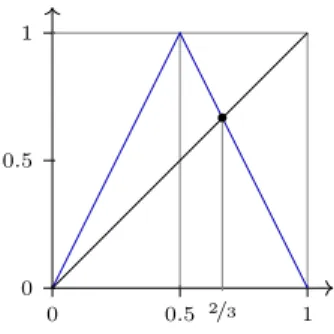
Section 1.4 Beyond non-expansive operators 7 0 0.5 1 0 0.5 1 • 2/3
Figure 1.4 – The ‘tent’ map (in blue). 0 and2/3are its two fixed points.
As a consequence, for an ergodic operator, the asymptotic throughput is almost surely constant, equal to a mean in space.
A reference on ergodic theory is the book of Cornfeld [CFS12].
Counters of the dynamics of Petri nets are determined by more complex operators, involving time shifts. However, it was proved that, with classical routing rules (pre-allocation, fluid ap-proximation of Bernoulli routing), such operators are monotone, non-expansive, and, with some additional constraints, the dynamics usually converges towards an asymptotic value, possibly infinite, independent of the initial conditions. See Cohen, Gaubert and Quadrat [CGQ95] and Gaujal and Giua [GG04b]. In stochastic settings, ergodic theory, together with monotonicity properties, often helps to determine the convergence towards asymptotic throughputs. See for example Baccelli and Mairesse [BM98] and Gaujal, Haar and Mairesse [GHM03].
In contrast, when allowing priority routing in Petri nets, the operator of the dynamics becomes non monotone: a token entering later in the system can pass by a token which entered before. The classical results obtained on Petri nets with monotone operators do not apply in this situation, and we need to investigate the behavior of non monotone operators.
Non monotone operators The following example, developed by Farhi, Goursat and Quadrat [FGQ11], shows that the general non monotone case is more complicated, even for an additively homogeneous, ergodic operator.
Let T : R2 → R2 be given by T (x
1, x2) = (x2, 3x2− 2x1∧ 2 + 2x1− x2), where ∧ stands
for a min operator. The map T is 1-homogeneous, and therefore, its analysis can be reduced to analyzing the operator ˆT in the projective space R2
/R (with ˆy = y2− y1):
ˆ
T (ˆx) = 2ˆx ∧ 2(1 − ˆx) . (1.2)
This is the (well-known) tent map, depicted in Figure1.4.
It admits two fixed points, 0 and 2/3, which are, therefore, eigenvalues of T . Moreover,
ˆ
Tk(x), with x any number with a finite binary development, reaches 0 after a finite number of iterates: thus, a dense set of initial conditions of [0, 1] is such that ˆTk(x) converges towards 0. However, neither 0 nor2/3corresponds to a mean asymptotic value of ˆTk(x)/k, independent of the initial conditions. In fact, the trajectory of ˆTk(x) is chaotic for any irrational number. In addition, for the Lebesgue measure, the unique invariant sets are sets of measure 0 or 1. Therefore, ˆT is ergodic, and the asymptotic cycle time ˆTk(ω)/k converges almost surely towards the mean value of ˆT , that is,1/2. We refer to Collet and Eckmann [CE09] for a more
detailed analysis of the tent map dynamics.
Hence, for non monotone operators, the asymptotic cycle time can be different from the eigenvalues of the operator.
A motivation of our work is thus to go further in the analysis of such non monotone maps resulting from Petri net dynamics with priorities.
Note that it is an open problem to construct a Petri net with priorities whose dynamics would be reducible to the tent map.
1.4
Contributions
We analyze the dynamics of discrete event systems with synchronization and priorities, by means of Petri nets and queueing networks. We apply this to the performance evaluation of the bilevel emergency call center described in Section 1.1.
Timed Petri nets are a convenient tool to model discrete event systems with complex con-currency phenomena. Their performance is measured in terms of their counters variables, counting the number of firings of transitions up to the current date. For restricted classes of Petri nets, like event graphs, the dynamics of these counter variables are known to be expressed by tropical (min-plus) linear equations, see Baccelli, Cohen, Olsder and Quadrat [BCOQ92]. Cohen, Gaubert and Quadrat [CGQ95] characterized the dynamics of a larger class of Petri nets, Petri nets with preselection routing, as a combination of max-plus linear and classical linear equations. From these counters equations, one can compute the asymptotic throughputs of a fluid approximation of the Petri net, using the techniques mentioned in the above section (Section 1.3). Convergence towards stationary regimes, whose throughputs are computed as solutions of linear programs, was shown in [CGQ95] for Petri nets having a positive Q-invariant, and in Gaujal and Giua [GG04b] in the general case.
Our approach in Chapter3builds on this series of results. A main novelty is that, while the previous models were limited to Petri nets with preselection routing, whose fluid approximation is in fact equivalent to the simpler class of choice-free Petri nets, we allow concurrency config-urations, in which tokens are routed according to priority rules. We show that the dynamics of Petri nets with free choice and priority routing can be expressed by piecewise linear equa-tions, leading to a rational tropical dynamics (3.3)–(3.7), thus generalizing the case of Petri nets with preselection routing. Moreover, we provide a complete proof of equivalence between the counters along execution traces of our Petri net, and the càdlàg, non-decreasing solutions of these piecewise linear equations (Theorem 3.1). We found our inspiration in the work of Farhi, Goursat and Quadrat [FGQ11], in which this modeling of priorities by rational tropical dynamics was applied to a timed Petri net describing a road traffic network.
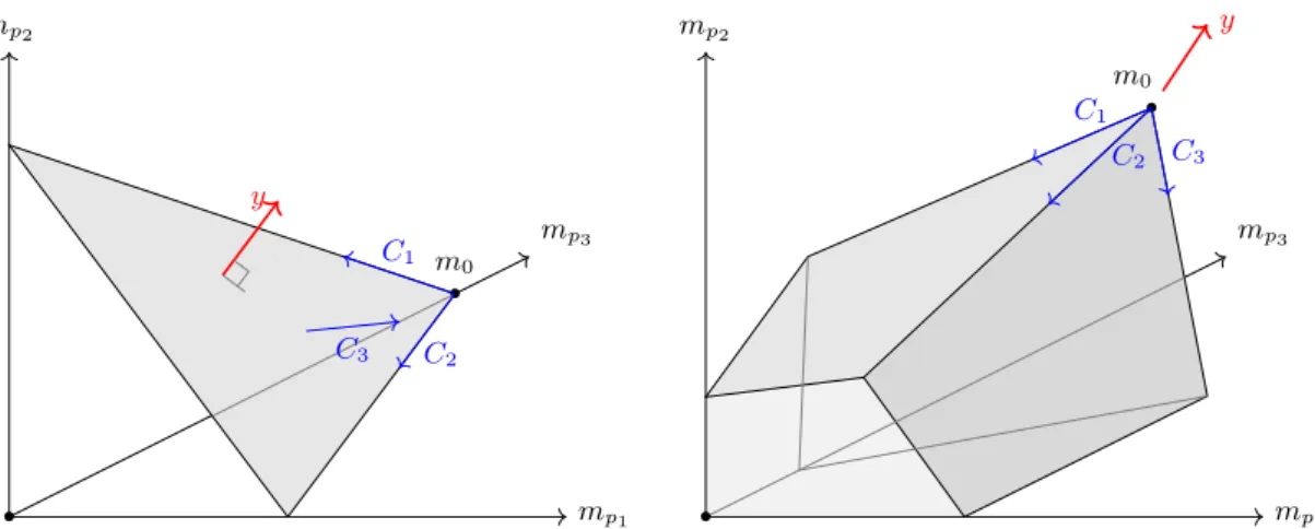
Like in the case of Petri nets with preselection routing, this allows us to investigate the asymptotic regimes. For the fluid approximation of the dynamics, we show that the affine stationary regimes of our class of Petri nets are precisely the solutions of a set of lexicographic piecewise linear equations, which constitutes a rational system over a tropical semifield of germs of affine functions: see Theorem 3.6.
However, because of the priority rules, the operator of our dynamics becomes non monotone (in a Petri net, a token having priority can pass by a non priority token), contrary to the preselection routing case. This has two drawbacks. Firstly, one cannot apply classical iteration algorithms, inspired by value iteration in Markov decision processes, to compute these affine stationary solutions. Moreover, our applications show that several affine stationary regimes may exist, for a given set of parameters, depending on the initial conditions (and they do not form a convex set), so that one has to enumerate all the policies of the net in order to determine the solutions. Nevertheless, expressing this problem as a rational system over a tropical semifield shows that it reduces to solving a tropical polynomial system, so that the asymptotic throughputs can still be computed.
Secondly, more fundamentally, the asymptotic regimes of this dynamics are not always the expected affine regimes. Numerical experiments show that periodic behaviors can be reached asymptotically, leading to different asymptotic throughputs. Such phenomena are occasioned by arithmetical relationships between the holding times. Thus, it can be considered as a pathology originating from our discrete time modeling.
The model investigated in Chapter 4 is therefore a continuous time one, designed so as to avoid the pathologies of the discrete time one. In this chapter, we provide an alternative, infinitesimal version of the dynamics described above, for the same class of Petri nets. In this setting, the dynamics becomes a hybrid dynamics, expressed by a system of differential equations, with a discontinuous right-hand-side. We require the variables of the Petri net to be
forward Carathéodory solutions of this hybrid system, that is, they are absolutely continuous
solutions of the system in its integral form, and left-accumulation of switching times is forbidden (this corresponds to our solutions being càdlàg functions).
Section 1.4 Contributions 9
same motivation as ours, that is, computing simple approximations of the behavior of a discrete Petri net. See also Vázquez et al. [VMJS13]. The main difference with our equations is that we model an infinitesimal equivalent of holding durations, while the original model of [DA87] rather considered enabling durations. Thus, the routing in this model was arbitrated by a race policy, while we can handle priority routing, in addition to preselection routing. Furthermore, this leads us to distinguish between tokens under processing and idle tokens in a place, and our dynamics become discontinuous, because the firing rate of a transition depends on the presence of idle tokens in its upstream place.
Our piecewise linear, piecewise continuous dynamics can be expressed as an infimum of linear dynamics, expressed in terms of policies of a Petri net. A policy associates with each transition a bottleneck upstream place, determining the flow of the transition when the policy reaches the infimum. One of our main results, Theorem4.9, is that there exists a unique forward Carathéodory solution for this dynamics. It relies on the constructive proof that, at any time, there exists a policy determining a valid solution on a forward time interval, and that this policy is unique, except for the case that another policy yields the same dynamics.
Similarly to the discrete time case, we exhibit the affine stationary regimes of this hybrid dynamics, see Theorem 4.11. We show in Corollary 4.12that they are the same as the ones computed in the discrete time case. Furthermore, numerical experiments tend to show that, unlike the discrete time model, stationary regimes are always reached by the Petri net dynamics, thus confirming the relevance of this model.
The idea of modeling a physical system by differential equations may seem remote from reality. Chapter 5 gives support to this modeling, by providing the proof that the dynamics of a stochastic, continuous-time network system, representing a bilevel call center, converges towards the same set of differential equations, up to an appropriate scaling of the system variables.
More precisely, the system considered in Chapter 5 is not a Petri net, but a queueing network, representing a bilevel emergency call center with only two classes of calls, urgent and non urgent. Level 1 operators answer all incoming calls, handle non urgent calls and transfer urgent calls to level 2 operators. If all level 2 operators are busy, then the level 1 operator waits with the urgent call, so that he is blocked until a level 2 operator becomes idle. The distribution of service times is exponential at each level, so that the corresponding stochastic process is Markovian.
For this model, under an appropriate scaling, we establish the convergence of the quantities of the system (fraction of blocked servers, fraction of free servers) towards asymptotic values ex-pressed as a piecewise linear function of the parameters of the system. The proof of convergence is technical, because reflection conditions at boundaries (depending on the presence of blocked operators at level 1 or idle operators at level 2) makes the analysis more complex. We resort to a scaling analysis (this kind of analysis was applied by Kelly [Kel91] to loss networks), which allows us to separate two regimes, one in which a fraction of level 1 servers remains blocked after some fixed delay with probability one, and one in which a fraction of level 2 servers is idle after some fixed delay with probability one. Interestingly enough, we show that, at the scaling limit, after some fixed time, the dynamics is solution of an ordinary differential system, corresponding to the dynamics proposed in Chapter4.
Finally, our three dynamical models, based on different semantics (see Table 1.1), applied to an identical physical system, lead to the same schematic asymptotic behavior, expressed as a piecewise linear system of the parameters, and describing the different congestion phases of the system.
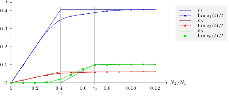
Regarding our bilevel emergency call center, under a saturation hypothesis, our asymptotic analysis allows us to identify three different congestion phases, described in Figure1.5, depend-ing on the ratio between the number of operators of level 2, N2, and the number of operators
of level 1, N1. Note that we suppose here that all level 2 operators have the same role. Going
from right to left, when N2/N1 is large, level 2 is sufficiently sized, and all calls are handled
at level 2. In an intermediate phase in which N2/N1 is between two critical rates, expressed
in terms of the parameters of the system, level 2 is congested, so that some urgent calls are not answered, but the extremely urgent calls are protected by the priority rule. In the lower
Discrete time Continuous time
Discrete firings Chapter3 Chapter5
(fixed processing times) (stochastic processing times)
Infinitesimal firings Chapter4
(hybrid dynamical system) Table 1.1 – Our three mathematical models in a nutshell.
PHASE 1 PHASE 2 PHASE 3 N2/N1 ρ level 1 throughput EU calls throughput U calls throughput ρ∗1 ρ∗EU ρ∗U r1 r2
Figure 1.5 – The three phases of the bilevel emergency call center with an homogeneous level 2, depending on the ratio between the number of operators at level 2 (N2) and the number of
operators at level 1 (N1).
phase when N2/N1 is small, level 2 is so congested that no urgent call is handled and that
the treatment of extremely urgent calls is slowed down. Because of the three-way conversation between level 1 operators and level 2 operators, level 1 operators are also blocked, waiting for level 2, and the throughput of level 1 is diminished.
In the unique chapter of Part II (Chapter 6), we focus on our case study of the Parisian emergency call center, and apply the analytical methods of Part I to a bilevel call center in which the second level is composed of different groups of operators handling different kinds of calls (police and firemen, in our case study). We also use simulations, which help us to present our results with a more operational point of view, and which take into account a certain number of characteristics of our call center that were not incorporated in our simplified model of Part I. Despite the operational advantages of this complex bilevel organization, a few situations are identified in which attention of practitioners is required. This is in particular the case of situations of “cross-congestion”, in which one of the groups of level 2 is saturated, and slows down level 1, because of three-way conferences. In such situations, all other groups of level 2 are also slowed down, because level 1 becomes bottleneck. This is an unwelcome side effect of this organization, but simple procedures can help avoiding such situations.
We also propose a statistical analysis of our emergency call center data (without entering too much into details), and point out a few additional observations derived from our simulations, as for example, the unavoidable trade-off between operators activity and calls abandonment. Calls abandonment could not be modeled by our Petri net class of Part I.
Part I
A Dynamical Analysis
Chapter
2
Preliminaries on Petri nets
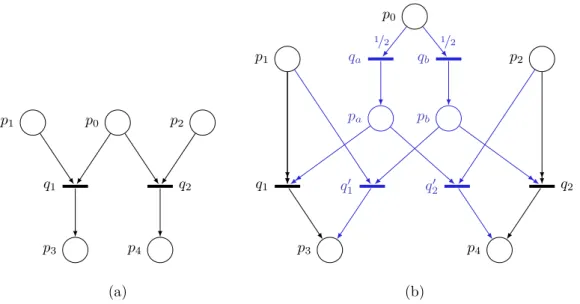
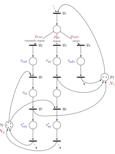
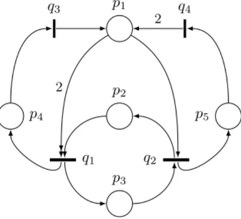
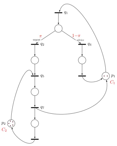
2.1 Untimed Petri nets . . . 142.1.1 General definitions of Petri nets . . . 14 2.1.2 Firing of transitions and Petri net dynamics . . . 15 2.1.3 Free choice Petri nets . . . 17 2.1.4 Fractioned firings: a relaxation of Petri nets . . . 17 2.1.5 External inputs and control . . . 18 2.2 Structural analysis of Petri nets . . . 19 2.2.1 An algebraic characterization of reachability . . . 19 2.2.2 Structural properties in the reachability polyhedron . . . 20 2.2.3 Minimal-support invariants of a Petri net . . . 21 2.3 Timed semantics of Petri nets . . . 23 2.3.1 Place and transition durations in Petri nets . . . 23 2.3.2 Differential Petri nets . . . 24 2.4 Routing rules in Petri nets . . . 25 2.4.1 Introducing routing rules . . . 25 2.4.2 Priority routing . . . 26 2.5 Three Petri net examples . . . 27 2.5.1 A simplified Petri net model of a two-level emergency call center . 28 2.5.2 The Petri net of Silva and Recalde (2002) . . . 30 2.5.3 The equivalent Petri net model of Chapter5 . . . 30
The objective of this chapter is to recall some basic definitions, notations and properties about Petri nets. In addition to the original model of Petri nets, we also develop some well-known extensions of this model that will be used or mentioned in this work. We try to propose a few relevant references for each of these extensions.
Going through all these notions and definitions (Sections 2.1, 2.2, 2.3), we arrive to the notion of routing rules, and introduce the one which is central to this thesis, priority routing (Section2.4).
Finally, we propose three Petri net examples in Section2.5. The first two ones will serve as applications of the results in Chapters3and4. The third one is an equivalent of the queueing network examined in Chapter5.
2.1
Untimed Petri nets
The modeling language of Petri nets was introduced in the beginning of the sixties by Petri [Pet62]. It was thought as a formal tool, aimed at modeling systems encountering concurrency and parallelism, and, therefore, convenient for practical applications such as manufacturing processes, communication networks, chemical reaction networks, and, more generally, processes where countable resources circulate between different places, encountering “joins” (rendez-vous, or synchronization), “forks” (splitting or branching) and “merges” (additions).
By the analysis of a Petri net, one would like to understand the behavior of a physical system, identify the critical paths of resources, the possible deadlocks and unexpected states, and provide guarantees of a “well-behaved” design.
We start by recalling the basic definitions of Petri nets.
2.1.1
General definitions of Petri nets
IDefinition 1. APetri netis a triple (P, Q, F ), consisting of a finite set P, whose elements are called places, a finite set Q whose elements are called transitions, P ∩ Q = ∅, and a mapping F : (P × Q) ∪ (Q × P) → N which indicates multiple directedarcsbetween places and transitions. F (p, q) defines the number of arcs from place p to transition q, and F (q, p) defines the number of arcs from q to p.
The mapping F of a Petri net is fully characterized by two P × Q matrices of natural integers, denoted by C+ and C−, such that the (p, q) entry of C+ is F (q, p), indicating the
number of forward arcs from transition q to place p, and the (p, q) entry of C− is the value
F (p, q), indicating the number of backward arcs, pointing to transition q, from place p. We call C+theforward matrixof the Petri net and C−itsbackward matrix. Note that the ordering
of the columns and rows of C+and C−entails a numbering of places and transitions: we usually
note transitions q1, q2, . . . , q|Q|, and places p1, p2, . . . , p|P|, according to this ordering. Owing to
the equivalence between F and the pair C+, C−, a Petri net can equivalently be defined by a
tuple (P, Q, C+, C−). Note that, in the Petri net literature, one often encounters the notations
Post (or W+) and Pre (or W−) to designate, respectively, the forward matrix and the backward matrix. Equivalently, one also often consider F (x, y) as thevaluationof a single (x, y) arc.
For two elements x, y ∈ P ∪ Q, we note x → y if F (x, y) > 0, and say that y is a forward neighbor of x, and x a backward neighbor of y. The set of backward neighbors of x is denoted
xin := {y ∈ P ∪ Q | F (y, x) > 0} and its set of forward neighbors is xout := {y ∈ P ∪ Q |
F (x, y) > 0}. For a place p, sets pin and pout are subsets of Q. The set pinis called the set of
inputtransitions of p, and pout the set ofoutputtransitions of p. Similarly, for a transition q,
sets qin and qout are subsets of P. The set qin is called the set of upstreamplaces of q, and
qoutis called the set of downstreamplaces of q.
We call self-loop the situation where a pair (p, q) has at least one backward arc and one forward arc. ApurePetri net is a Petri net without self-loops, i.e., where the existence of a (p, q) arc and of a (q, p) arc are mutually exclusive. This is equivalent to having min(C+, C−) = 0 (by
the minimum of two matrices or vectors, we mean the matrix or vector composed of entrywise minima). For pure Petri net, we define theplace–transition incidence matrix, or, for short, theincidence matrix C := C+− C−. A matrix C ∈ (N ∪ −N)P×Q uniquely determines the
matrices C+ and C− of a pure Petri net by C+ = min(C, 0) and C− = min(−C, 0), so that a
triple (P, Q, C) defines a pure Petri net.
I Definition 2. A marking of a Petri net is a mapping m : P → N. A place such that m(p) > 0 is called amarked place. For such a place, we say that m(p) designates the number oftokensof place p. We equivalently describe a marking as a column vector of NP. Amarked
Petri net is a pair (N, m0) where N is a Petri net, and m0 a marking, called the initial
marking of the marked Petri net.
Bystateof a Petri net N , we mean a given marking m ∈ NP.
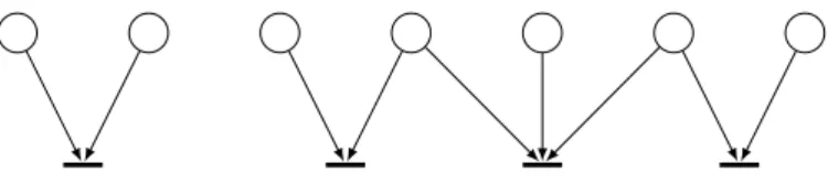
The following conventions hold for graphical representation of Petri nets: places are depicted by circles, transitions by rectangle or thick segment lines, and directed arcs link places to transitions, and vice-versa. Multiple arcs can equivalently be depicted by arcs with an integer valuation. Finally, tokens are represented by dots inside the circles of the places. See Figure2.1.
Section 2.1 Untimed Petri nets 15
2
Figure 2.1 – A Petri net with three places and a transition. Despite the three tokens in one of its upstream places, the transition is not fireable, because its second upstream place is empty. A firing of the transition would produce two tokens in its downstream place.
A Petri net isconnectedif it is connected as a bipartite graph. Asubnetof a Petri net is defined by P0, Q0, C0, where P0 ⊆ P, Q0is the set of transitions of Q having at least one arc to or
from P, and C0= C|P0,Q0, that is, C restricted to its entries in P0× Q0. A non connected Petri net can be described by the partition of its maximal connected subnets. The absence of arcs between two of these maximal connected subnets implies the absence of relationships between them. Therefore, in the following, without loss of generality, we only consider connected Petri nets.
2.1.2
Firing of transitions and Petri net dynamics
The dynamics of a marked Petri net describes the evolution of its marking under firings of transitions.
For a matrix A of dimensions P × Q, the notation Aq with q ∈ Q stands for the q-th column of A. The notation Ap,q with p ∈ P and q ∈ Q stands for the (p, q) entry of A.
IDefinition 3. Let N = (P, Q, C+, C−) be a Petri net and m0 be a marking. We say that
transition q isfireablewith m0if m0> (C−)q (the notation (C−)q designates the q-th column
of C−, so this is a entrywise inequality on two vectors of NP), that is, if for each upstream place
p of q, the marking of p is larger than the number of arcs (p, q).
A transition q firesin state m to state m0 if it is fireable with marking m, and if
m0= m − (C−)q+ (C+)q. (2.1)
We use the notation m−→ mq 0.
The firing of a transition consists in decreasing the marking in upstream places and in-creasing the marking in downstream places, in quantities given by the backward and forward matrices. We say that transition q consumes (C−)p,q tokens in each upstream place p and
produces(C+)p0,q tokens in each downstream place p0.
We now define a firing sequence as a sequence of firings of transitions, such that the (k+1)-th transition is fireable for the marking reached after the firings of the k first transitions.
IDefinition 4. Afiring sequenceσ for marked Petri net (N, m0) is a word on transitions
σ ∈ Q∗, that satisfies the following, inductive, rules:
m−→ mε 0 if m = m0
m−→ mσq 0 if ∃m00∈ NP : m−→ mσ 00−→ mq 0,
where σq is the word composed of the prefix σ and the letter q, and ε is the empty word. We say that the firing sequence σreachesmarking m0 from m if m−→ mσ 0. We also speak
of a firing sequence of a marked Petri net as anexecutionof the marked Petri net.
In discrete Petri nets, one is typically interested in describing the reachable markings of a Petri net, that is, the markings that can be reached by some sequence of transitions.
IDefinition 5. Let (N, m0) be a marked Petri net. A marking m is said to bereachablefor
(N, m0) if there exists a firing sequence σ such that m0
σ −→ m.
If m is a reachable marking of (N, m0) and σ a firing sequence from m0 to m, we denote
by |σ| the vector of NQ counting the occurrences of every transition in σ, that is, |σ|q is the number of occurrences of q in σ. Vector |σ| is called theoccurrence count vector, or Parikh
vector, or commutative image of σ. The markings m0and m are related to |σ| by the following
result:
I Lemma 2.1. Let (N, m0) be a marked Petri net and let m be a reachable marking of m0,
with the associated firing sequence σ. We have:
m = m0+ C|σ| . (2.2)
This equation is called the fundamental equationof the Petri net.
Given two markings m and m0, the existence of an x ∈ NQ such that m0 = m + Cx is a necessary, but in general not sufficient condition for m0 to be a reachable marking of m. Moreover, if m0 is a reachable marking of m and if x satisfies the equation m0= m + Cx, there does not necessarily exist a firing sequence σ with m →σ m0, whose occurrence count vector would be x.
Proof. Equation (2.1) can be written m0= m + Ceq, with eq the vector of dimension |Q| such that (eq)q = 1 and (eq)q0 = 0 for q 6= q0. One proves by induction on the length of σ that
m0 = m + C(P
q∈Q|σ|qeq). J
The following properties are related to the notion of reachable markings and firing sequences: IDefinition 6 (Basic properties of a Petri net). Let (N, m0) be a marked Petri net.
• A transition q isdeadif there does not exist a firing sequence σ such that σq is a firing sequence from m0.
• A transition q is live(or strongly live) if for every reachable marking m, there exists a firing sequence σ such that σq is a firing sequence from m.
• A reachable marking m of (N, m0) is a deadlockif no transition is fireable at m. If no
reachable marking of (N, m0) is a deadlock, then (N, m0) isdeadlock-free.
• A place p is k-bounded if, for any reachable marking m, m(p) 6 k. It isboundedif there exists k such that it is k-bounded.
• If every transition of (N, m0) is dead, we say that the Petri net isdead. This is equivalent
to saying that no transition is fireable for m0.
• If every transition of (N, m0) is live, we say that (N, m0) is alivePetri net.
• If every place of (N, m0) is bounded, we say that (N, m0) is aboundedPetri net.
Characterizing the reachable states of a Petri net has been an important problem in Petri net theory for decades. It was observed that many other problems on Petri nets reduce to this reachability problem [Hac76]. We owe to Mayr [May84] and Kosaraju [Kos82] a major theorem in this respect: the reachability problem for Petri nets isdecidable, that is, that there exists an algorithm that answers if, for a marked Petri net (N, m) and a vector m0 ∈ NP, m0is reachable
from m (and returns a firing sequence σ such that m →σm0). The proof builds on the results
of Karp and Miller on vector addition systems [KM69], which where shown to be equivalent to Petri nets. However, the reachability problem is EXPSPACE-hard [Lip76]. See also the recent algorithm of [FL15].
Reachability is just one of many useful Petri net properties. One would for example like to know if a Petri net is bounded, if some marking is a home state, if a marked Petri net is live, or deadlock-free, or persistent. One would also like to know if a given Petri net reachability set has some specific structure, for example, if it is a language or a semilinear set. We refer to the overview of Esparza and Nielsen [EN94] for decidability results (and definitions) of such properties, for various subclasses of Petri nets. Many of these problems reduce to the reachability problem.
We point out that these results build on the analysis of some structures associated with Petri nets, such as the reachability graph of a Petri net, its coverability graph (see definitions in [Mur89]), or its occurrence net (introduced in [BD90]).