CONTINUED DEVELOPMENT OF NODAL METHODS FOR NUCLEAR REACTOR ANALYSIS
by
A. Henry, A. Dias, W. Francis, A. Parlos, E. Tanker, and Z. Tanker
CONTINUED DEVELOPMENT OF NODAL METHODS FOR NUCLEAR REACTOR ANALYSIS
Final Report for the Period March 1985 Through June 1986
Project Director: A. F. Henry Work performed by: Antonio Dias
Winston Francis Alex Parlos Ediz Tanker Zeynep Tanker Energy Laboratory and
Department of Nuclear Engineering Massachusetts Institute of Technology
Cambridge, Massachusetts 02139
Sponsored by
Northeast Utilities Service Company Pacific Gas & Electric Company
under the
M.I.T. Energy Laboratory Electric Utility Program M.I.T. Energy Laboratory Report No. MIT-EL-86-002
Table of Contents Page No. Table of Contents ... Acknowledgments ... ii Foreword ... iii Introduction ... 1
1) Transport Effects Accounted for by a
Finite-Difference Diffusion Theory Model ... 3 2) Standard Nodal Codes Derived
Systematically ... 13 3) Development of a More Efficient Flux
Reconstruction Method for BWR's ... 57 4) Development of Methods to Analyze
Transients ... ... 58 5) Time Integration Schemes for the Point
Kinetics Equations ... 73 References ... 80
Acknowledgments
The work described in this report was supported by Northeast Utilities Service Company and Pacific Gas and Electric Company under the MIT
Energy Laboratory Electric Utility Program. We wish to express our thanks for that support.
Foreword
The physics design of nuclear reactors is today carried out, almost exclusively, by the application of numerical models that describe neutron behavior in a core throughout its life history. It is accordingly very important that the models used be accurate and reliable. At the same time, they must not require exorbitant amounts of computing machine time.
The present report is a summary of a third year of effort in an on-going program to improve such mathematical models. The development of improved procedures for analyzing static problems (including depletion and fuel management) has been quite successful and is now largely complete, and present concentration is on applications to transient analysis. Im-plementation of the methods developed into production computer programs that fit into presently used packages remains as the most important outstanding requirement.
Introduction
The development of computer programs that predict neutron behavior in nuclear reactors falls into three stages.
The first stage involves the derivation of the basic equations that constitute the model. These are best found by systematic reduction from a more accurate model so that the physical and mathematical approxima-tions made can be understood clearly.
Next it is necessary to create a computer program that solves the model equations and to test its accuracy by comparison with reference calculations.
Finally, it is necessary to fit the tested model into standard pro-duction codes. It is really only when this last stage is complete that utilities can take advantage of the improved accuracy and efficiency of the newer models.
The MIT development is now reaching this final stage. Production codes based on the nodal code QUANDRY developed at MIT are now coming into use. These include the nodal option QPANDA of SIMULATE-3 developed by Studsvik of America, the STAR program developed at N.U.S., and the ARROTTA code developed at S. Levy for EPRI.
Some of these organizations have undertaken development work which might have been carried out at MIT. For examples, both
Studsvik and N.U.S. have successfully incorporated into their nodal
codes an improved iteration scheme (suggested by Kord Smith) which reduces computer storage requirements substantially. In addition, Studsvik is providing a direct link between CASMO and QPANDA which avoids entirely the need to run any fine-mesh PDQ problems -- either assembly-sized or quarter-core -- in order to obtain homogenized nodal parameters. Finally, Temitope Taiwo, working at Northeast Utilities, has reprogrammed QUANDRY to solve for the nodal adjoint fluxes.
Since complex production-type programming efforts of this nature are better carried out by organizations where the personnel
are not continually changing (as happens with graduate students), we were pleased to be able to drop these items from our agenda. Instead, we have continued to concentrate on the development and preliminary testing of accurate and efficient methods for predicting neutron behavior in LWRs. Accomplishments of the past year are described in the sections below.
To summarize briefly:
1) We have completed the development and testing of a method for determining fine-mesh, finite-difference, diffusion theory
parameters (such as are used in PDQ) that reproduce quite accurately the criticality and power distribution produced by transport
spectrum codes such as CPM or CASMO.
2) We have shown how to derive the adjustable parameters required by the standard nodal codes FLARE and PRESTO directly from a QUANDRY calculation.
3) All the necessary computer codes for testing a new scheme for reconstructing detailed pin-power distributions from QUANDRY solutions for BWR's have been completed.
4) A one-dimensional, two-group scheme for analyzing transient neutron behavior has been derived systematically from the QUANDRY,
three-dimensional nodal equations. Coding is substantially complete, and testing has begun.
5) New time-integration schemes for solving the point
kinetics equations, which permit the use of large time steps, have been developed and tested.
1. Transport Effects Accounted for by a Finite-Difference Diffusion Theory Model
We have completed the development of a systematic method for deriving few-group, fine-mesh, finite-difference diffusion theory parameters from multi-group, transport theory calculations carried out for an entire assembly.
A discussion of the theory along with a number of numerical test cases is given in MIT-EL-85-002, 1( ) and Reference (2) is a complete report of the work done on the method.
Face-dependent discontinuity factors for the pin-cells are initially introduced to reproduce the transport results exactly. With adjustments made for fuel cells adjacent to control rod fingers
or burnable poison cells and for cells adjacent to the reflector, the face-dependent discontinuity factors can be replaced with approximate average values, and then, by a renormalization of the
two-group cross sections, can be made to disappear entirely. Thus, the standard finite difference code, PDQ, can be made to reproduce rather closely all the reaction rates determined by transport theory. Maximum errors in pin-power (relative to reference calculations) were under 2% for our test cases. Since the adjustments for cells next to a control finger or poison pin or reflector can be made automatic, the method is more straightforward than the trial-and-error procedure currently used by most utilities. Also, since all reaction rates are matched (rather than just
absorption in burnable poison pins or control fingers, it is expected to be more accurate.
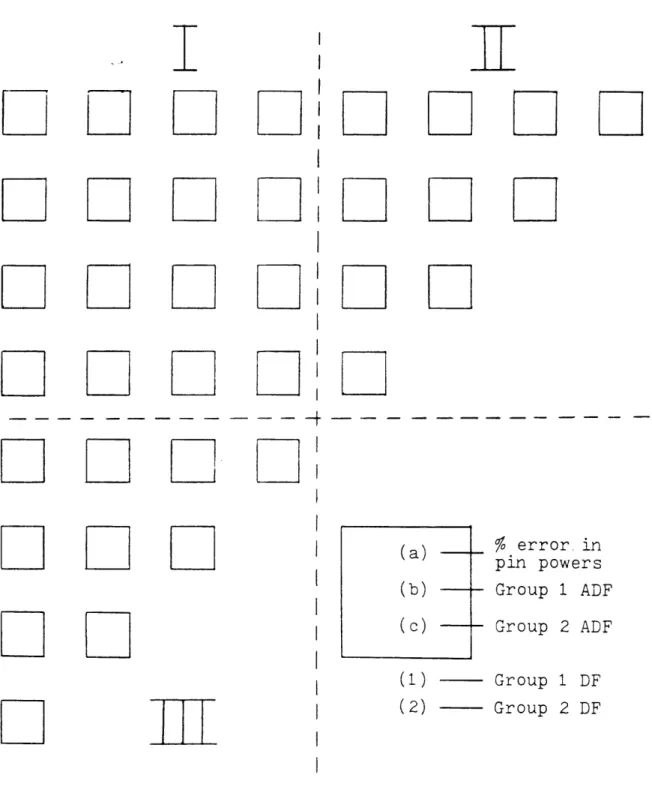
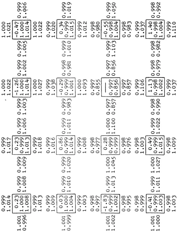
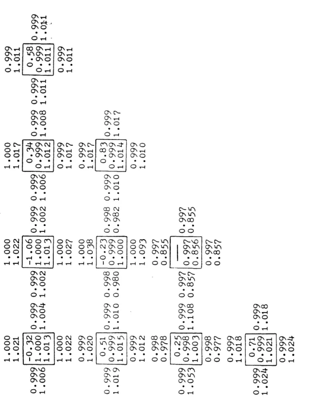
To illustrate the method for a difficult case, we consider the rodded assembly shown on Figure (1-1). The black squares represent fuel-pin-sized regions occupied by control rod fingers. Figure (1-2) shows an eighth of the assembly partitioned into three zones along with the legend for Figures (1-3), (1-4) and (1-5). These latter figures show, for the three partitions, the error in pin power when the "(3+1)" approximation (explained below) is used along with the average group-1 and 2 discontinuity factors and the
face-dependent, group-1 and 2 discontinuity factors for each pin-sized region. The face-dependent discontinuity factors were found by requiring that "exact" finite-difference type equations with one mesh-square per pin-cell and incorporating three
discontinuity factors (Ref. 1) reproduce reference results for the pin-cell-averaged group-fluxes. (For both reference and approximate
m m rnr rn-m mm
im
l n -m PlIEI
_ m I I _ - mW
-mI
_ _ _ _ _ _ i i~
i ImEl
_ _ I__ _ _ _i
_ _-_
_ I_ _ 21 ndismnsions
of
"ch -S11
L.4 =n
by .4
m3
Fig. 1.1 Heterogeneous PWR Assembly Geometry
r
m m m m m m m mmmK
I
OMM" i I I .l ---I I I m lm m-m-_
m m m m T m m mm_ m .m . m _ mm m m~~~~~~~~~~~~ m m---
~~~~~----2/~-I mmmmm mmmmm I I I mm mm mm mm I I r I iI
tI
II
l
t
I
I--
I
I
1
Ioooo
i
1
DLZ~iIJ
1
DDDD
DDDD
~ ~~~~~~~~~~~~~~~~~~~~~~~~~~~~~~~~~~~~~~~~~~~~~~~~~~~~~~ID
DDDD'DD~~~~~~~~~~~~~~~~~~~~~~~~~~~~~~~~~~~~~~~~~~~~~~~~~~~~~~~~
DDDD~~~~~~~~~~~~~~~~~~~~~~~~~~~~~~~~~~~~~~~~~~~~~~~~~~~~~~~~~~~~~D~~~~~~~~~~~
L L C-X
O~ 1
[
DDDD
O
III
%
error in
pin powers
-
Group 1 ADF
-
Group 2 ADF
(1) Group 1 DF (2) Group 2 DFFig.
(1-2) - Rodded reference discontinuity factors, (3+1)
averages rand
the errors in pin powers
(a) (b) (c) -I I I I I I I I I I I I I
ON -400-d
ON
00
OO
00100
0,-4
00
o
r\ o ONO 0 O 000" · 00 0",0O ..
O 0
0\ t
a'o
0C\ o * o' 4 O\\O ('\ O 01\ow'
O · G\ O~ O\ O*00
\
00
O 00,o
0 0
O a\
O 0a,-,
0\0
*\
O
0\ n
O
O
C\ 0\
QO -.4 0 -4 · \0 · \0 · N \ O 0 0 O CC) Cr\o o
cn -- '-OC Oo O
0C\ \ ·\
0
O O Ocr N -4 O'\ \ O o\ O000
-OO O 0\O
0 -_4O O'co I\ 0\ 0 C\ 0 Ocr 0,\ C'\ Vr~0\ 0
O'00 1 OOC\ ·\ .I ·c\ 000 I
00
O\0
C7\ U00
O 00,-oC\
U-)
00
00
,, u
00
O
0
O o-C\ cot- 0CN(DI O'c- CO',00N \ .\O · -\o'
Oo
00
00
o-r04
0 0
-4 -4o o
0 -4 coI-0\
0\
00
o a'o
0
o
I O O Oo o
* $00
n 0\000 0
O Oac
u
00
co\'0\0
O Oo\ o'
owo
0
Cr00 01 0\Q7\
0 ,.0\0
* 0O
o\\OO\ o
*' -O H40 O
0\ 0 O O -4 O\ O0\0
c o
00
O\ O\ 0 O00-a'o 1-4
o-O N
0 0
\ 0\
0 0
0,-l
O'\ -0 O 0'\0-4
0\
OO
* -O -O, 0\0 OO
I-4 0 O O O O0- O
-0\0
·
\0
0\0
0w-i
o c 0 0',oo
0\
O o · o or O· 4 ..-~- * O o
Lt J
O- 0O-- .· 0- O.. O c ··* 0 -4 o 0o 0.. .
O0\\O
03
o
ONO
(
CO
'N
o
'
ONO * 0 , n- o. 0 0 oo o o \ cr\ .o\0
0 0
oo
ON \ on
oc-
o
nco
o\0
cn
C)
C-\
C-c
O
N
o o
-
O N o n N CO
o o\
, 0
C\N)
o
* -. 4 I I I 0 0 o U S S- oO\l
co
0
C
ONO N\ co\ V * . S 5 0 0ao
Co~
0~4
00
-
00
oo
. oo 04
O N n0o
1- O 0 C\N\o
U)(-4Co
,o
4 CNVo
Qo n
.o
\00 C \0 . Ct
C O N,
-4O I O -- O- -4 O O,-- * O O O O , O,0,- O,-I
0NO OO O - O O
O
Fig (1-4) cont'0d
O
- Partition
O,-
II0
Oa-
0
Co
O\ O
ON\O OiO OcO
0 00
oo
\
\,-0-. 4 0-4\O
*CO
0N
.O
00
0
00 0
-
0
-
0 4
0
0",
T:
0 "
,
0,-4 o N ON- cr OO0 Oo0 0
CO
0
O
7 c- cr\ o zt O0 c6 ON o 6 6 o \ *O00 0 0 C0,-O
O.
-0
OC,1 0\ O 0\ O ONc00
0o
O
O
0O
O\ 0
O 0
,
0
0\
0
0.
00
I-
O
O
iO
00 -
N
00
00
coo
0
c'
O 0
a
ONo 0o
O0
00
0 .00 ONO
*ON
00
*00 0
ON0 O0 O0
.. O * . . . C: .O . 0 . ... O . .. .. ..
ON CC 0 N CO\\O
* 0\ 0 O 0\ 0\0
0 0\
0 C
O 0\
C O
,-40 -4 -4 0 0
assembly calculations, zero-current boundary conditions were applied over the entire surface of the assembly.)
As shown in Ref. (1), if the face-dependent discontinuity factors are replaced by their cell-averaged values and if the homogenized diffusion coefficients and cross sections for the pin cells are divided by these average values, a set of finite
difference equations similar to those used for standard design (PDQ) is obtained. Thus, insofar as face-dependent discontinuity factors may be replaced by average values, PDQ can be made to match CPM or CASMO results by a straightforward, one-step procedure.
Unfortunately, Figures 1-3), (1-4) and (1-5) show that, for the fuel-pin cells adjacent to rodded cells, the group-2 discontinuity factor for the face nearest the rod-finger is significantly higher than those of the other three faces. Thus, replacing the
face-dependent, group-2 discontinuity factors of fuel-pin cells adjacent to rodded cells by average values is likely to be a poor approximation.
We have developed two methods to circumvent this difficulty. The first is to average (for fuel-pin cells adjacent to a rodded cell) the thermal discontinuity factors for only the three faces furthest from the rodded cell and to use the actual face-dependent value for the faces nearest the rodded cell. This is the "(3+1)" approximation.
The second scheme is based on the fact that what appears in the "exact" finite difference equations is the ratio of the
discontinuity factors on the two sides of that interface.
Examination of Fig. (1-3) shows that the face dependent, group-2 discontinuity factors for the rodded cell vary in the narrow range 0.855 to 0.857, and those for the faces which the four neighboring fuel-pin cells have in common with the rodded cell vary in the range 1.093-1.106. Moreover, for the four fuel-pin cells adjacent to the rodded cell, the averages of the thermal discontinuity factors for the three faces not common with those of the rodded cell vary in the range 0.999 to 1.004. It follows that if we reduce the thermal discontinuity factors of the faces adjacent to the rodded cell and those of the rodded cell by dividing by, say, 1.1, the ratio of discontinuity factors across faces will be unaltered, but the values of all four thermal discontinuity factors for fuel-pin cells
adjacent to the rodded cell will be much closer to each other, so that replacing them by their average value will be a much better approximation. We call discontinuity factors altered in this manner "adjusted discontinuity factors."
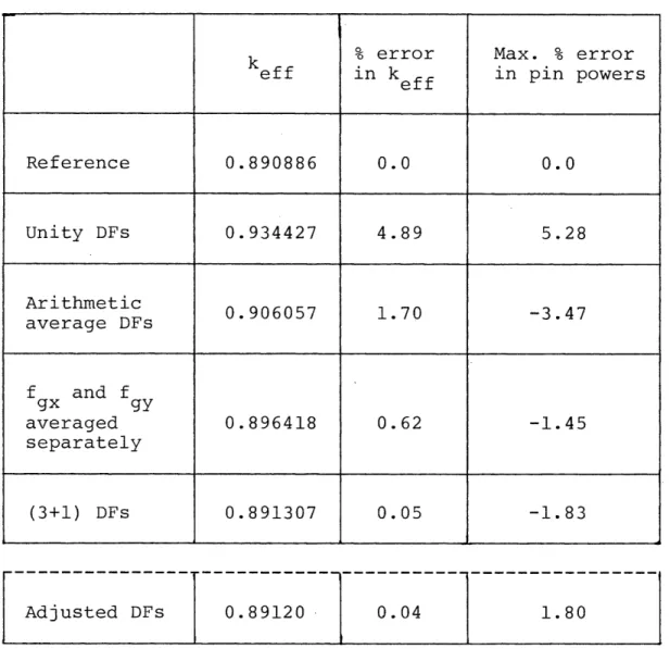
Table (1-1) shows the difference from reference results due to the use of various averaging procedures applied to the discontinuity factors of the pin-sized-cells comprising the assembly of Figure
(1-1). Clearly, using unity-valued discontinuity factors (no correction) leads to unacceptable errors in both eigenvalue and pin-power. Straight arithmetically-averaged discontinuity factors do little better. (Tests presented in Ref. (1) show that
% error
Max. % error
eff in k in pin powers
eff
Reference
0.890886
0.0
0.0
Unity DFs
0.934427
4.89
5.28
Arithmetic
0.906057
1.70
-3.47
average DFs
f and f gx gyaveraged
0.896418
0.62
-1.45
separately
(3+1) DFs 0.891307 0.05 -1.83Adjusted DFs
0.89120
0.04
1.80
holes rather than control rod fingers are present.) Use of separate averages for the x and y directions leads to the smallest error in predicted fuel-pin power, but an unacceptably large error in
eigenvalue. On the other hand, both the (3+1) and the "adjusted" discontinuity factors do well.
Since the "adjusted" DF's can be made to disappear entirely by renormalization of the pin-cell cross sections, we recommend this as the favored method for forcing a match between PDQ and codes like CPM or CASMO.
2. Standard Nodal Codes Derived Systematically - Winston H. G. Francis
Standard nodal codes such as EPRI-NODE-P/B, FLARE or PRESTO usually require that certain adjustable parameters and albedos be determined by fitting to quarter-core PDQ results. Under the assumption that the discontinuity factors (6 per node, per energy group), which make fluxes predicted using the coarse mesh finite difference (CMFD) QUANDRY equations match exactly those obtained by the regular QUANDRY equations, can be replaced by one, average value per group, we show below that these standard models can be derived
directly from QUANDRY. If this basic approximation is valid,
"coupling constants" and albedos for the simple models can be found in a direct, non-iterative fashion.
To show how the fitted parameters of standard nodal schemes can be found directly from a QUANDRY solution, we shall first derive two of them (FLARE and PRESTO) in a standard fashion. Then we shall
show that, by using node-face-dependent discontinuity factors,
finite-difference equations capable of reproducing reference QUANDRY results can be derived. The face-dependent discontinuity factors will then be approximated by node-averaged values, and the fitted parameters of FLARE and PRESTO will be found in terms of these averaged-values. Finally, we shall present some preliminary tests of the systematically derived FLARE and PRESTO models.
2.1 SEMI-EMPIRICAL NODAL METHODS
Semi-empirical nodal methods may be derived from the following
(3) multi-group equations V.J (r) + tg(r) g(r) (2.1) G g'= 1
1
X
E,(r)
+
(r)
] g,(r)
where the notation is conventional.
We consider a node (i,j,k), with a horizontal mesh spacing h in both
the x- and y- directions, and a vertical mesh spacing k in the z-direction. By integrating over the volume of the node (i,j,k), and using Gauss' theorem, we obtain 6 JS g(-r)-nS dS + h2k i,j,k i,j,k m=l m G =hk 2 1 ik i,j,k] ij,k g' =1 g = 1,2,...,G. (2.2) We also such that all which case
i,j,k = O 12
divide the energy spectrum into two groups by setting G = 2, fission neutrons are introduced into the fast group only, in X1 = 1 and X2 = 0, and there is no up-scattering , i.e. For simplicity a generalized node (i,j,k) will be represented
by a single index "p", so that the resultant two-group equations are:
6
6| (r) -n dS + h k 1 =
[
uEl + VEf2 (2.3a)r
|S J2(r)nS dS + h 2k P = h2k P2 (2.3b) where1 tl 11' and 2 t2 22
In the second (thermal) group, the leakage term is generally much smaller than the absorption term, and hence may be neglected. The result is the one-and-a-half group approximation. Alternatively, in order to maintain a formally exact scheme, we can define a parameter B , such that
6 m=l m so that '2 D B2 2 (2.5) 2 DP + P 2 2
The advantage of introducing B of introducing B will be will be apparent later, and obviously by P
setting B = 0, we can return to the one-and-a-half group approximation.
P
reduced the problem to a one-group model, in which we only have to consider the fast group explicitly.
6 2 Wp ns J (r)-n dS + h k[ fl f2 p ] p m=l m A 2
hk
Alcol
VEp kP = fl + co P where kP 00 P f2 21 P ( D 2 + P ) 1 2p 2 (2.6) (2.7)is the conventional infinite multiplication factor for a two-group model, with the materials buckling
'
~~~~~~~~m
(B2 ) replaced by B2P
FLARE MODEL
(4)
In order to derive the FLARE model , we now define a fission neutron source term for each node,
SP h2k P kP WP 1 c 1
so that Eq. 2.6 can be written
6 j Pq q-p XP SP SP kp [q=1 k (2.8) (2.9)
Rearrangement yields kP 6 SP co P j Pq [ (2.10) q-l kp 6 6 co - J SP + Sp (2 10)
q=l
q=l
A
By defining a kernel Wp q by the relation
WPq _p+
-
p
(2.11)
S
so that WP q represents approximately the probability that a neutron in node p in a reactor, which is artifically critical, will cross to an
adjacent node q, we may rewrite Eq.2.10 as
kP 6 6
SP c [ 1 WPq] S + WqP Sq] (2.12)
q=l q=l
which is the basic nodel equation in the FLARE model. In FLARE, the kernel Wp q is taken to be of the form
2 J(M2) M2
Wpq ( - g + g P (2.13)
2h h
where g is an adjustable parameter, and M2 is the migration area. P
According to this expression, Wp q depends only on the properties of node p, a condition which is obviously not true physically. The kernel was originally derived as a combination of a slab-diffusion kernel and a difference-equation kernel in a non-rigorous and quite arbitrary manner. However, by adjustment of the g-factor and the albedos, it is possible to reproduce a reference solution, i.e. eigenvalue A to < 0.5 % and the nodal powers to < 10%, which is considered satisfactory for initial design calculations.
PRESTO MODEL
The PRESTO model( 5 ) is a modified coarse-mesh finite-difference (MCMFD) model, which uses node-centred and face-centred point fluxes. The nodal volume-averaged flux is assumed to be approximated by
4 2
_p 3a p (1-a)/4q + R (2.14)
p 2 I +
pq
(2.14)3a+(l-a)(R+2) 3a+(1-a)(R+2) q =1
where 'p is the point flux at the center of node p, and 'Pq is the
center-point flux on the interface between nodes p and an adjacent node q, with "a" being an adjustable weighting factor. We note that when R = h2/k2 = 1, i.e. h = k
6
p
a
~
p ++
1-aq(2.15)
(2.15)pq q=lIntroducing the definition (2.7) into the fast group equation (2.3a) yields 6 X Jl(r)-ns dS = h 2k
[
k - 1 p kp (2.16) 1 SI
c 1 D1 "S m 1 m=l mwhere (P is replaced by P1 to distinguish point fluxes from nodal volume-averaged fluxes. In order to determine the left-hand-side, the net current on the interface between adjacent nodes p and q is assumed to be given by pq P (Pq _ P J ] h/2 q -q - Pq [D (2.17) h/2
With this assumption made, the surface fluxes and currents on the interface are pq DP WP + Dq (2.18) VP (2.18) DP + Dq pq 2 D p D q p (2.19) = - - ( P q (2.19) h Dp + D q
Hence Eq. (2.16) becomes 4 2
i
-hk) D ( q p ) + (h2 ) 2 D D q Pk D
+ D
q (DP
+
p ) qhl = qv= 1 h2k kP - 1 e s Pwhere the subscript for group-i has been dropped, so that
4 qh= 2 2k (q - P) -D + Dq qv-1 Dp q 2kR (P)q _
D
p+
D
q h2k kP 1 ] :p =h 2k I kP 1 [ 3a A 3a+(1-a)(R+2) I. WP + 2 (l-a)/4 [ Pq + R VPq 3a+(1-a)(R+2) l 1 v =1 q 1This set of equations, together with suitable boundary conditions, can be solved to yield the point fluxes P , from which the nodal-averaged
fluxes can then be reconstructed.
(2.20)
(2.21) n
2.2 SYSTEMATIC NODAL METHODS
The starting point of all nodal methods based on diffusion theory is the set of multi-group equations (2.1), which is repeated here
V-J (r) + g(r) g (r)
-g - tg-
g-G
=x·
|-g
VZC
g(r) + gg,(r)
p
,(r)
(2.22)
g'=l
We again consider a node (i,j,k), with a horizontal mesh spacing "h" in both the x- and y- directions, and a vertical mesh spacing "k" in the z-direction. Integrating Eq. (3.1) over the volume of the node (i,j,k), we again obtain 6 J (r)n dS + h2k i,j,k i,j,k S m tg g m=l m G 2
[1
i,j,k + i, j,k(2.23)k =h k %9 x ' ~g, (2.23) g'=l gl=1 g = 1,2,...,G.Since Eq. (2.23) contains two unknowns W i and J (r), we require
g g
-another relation between them, so as to form a closed set of equations. This relation is usually termed the "nodal coupling equation", and is mainly responsible for the differences in the various nodal methods.
ANALYTIC NODAL METHOD (QUANDRY-CMFD APPROXIMATION)
In the CMFD approximation, the nodal coupling equation is based on Fick's law of diffusion
I
Jgx(xi+lY,Z) dy dz hk i+l,j,k g _ _Di+l,j ,k g _ Di,J ,k g fi+l,j, kJ
f
g(Xi+l,y,z) dy dz gx-h/2 fij,k | | g(Xi+l,y,z) dy dz - hk i jk gx+ h/2 (2.24)where because of the introduction of the discontinuity and fi,j,k these are now formally exact relations.
gx+
way, Equa. (2.24) defines formally exact values for factors.)
Eliminating the face integrated surfaces from Equa.
factors fi+l,j,k gx-(To put it another the discontinuity (2.24) yields
I
T
Jgx(xi+l y,z) dy dz Di,j,k Di+l,j,k=-2k
g
g
fjk
Ii+l,j,ki+ljk
fi,j,kDi+l,j,k + fi+l,j,kDi,j,k gx- g gx+ g gx- g -i+l,jk i k x- -1 = 2k - gx- ,j,k gx+ filj,k i+l,j,k Di+l,j,k ,j,k gx- g g gICjk
i,j,k
gx+ g f- ik i,j,k1
gx+ g J (2.25)Similar expressions can be obtained for
Jgy (x,y z zz) dx,
gy j+1l' etc. By introducing these expressions into
equation (1.24), the QUANDRY-CMFD equations are obtained,
-
i+l,jk
fijk -
-1
-
2k
gx-
+gx-+
fi+l,jki+l,
jk fj
kijkk
Di+l,jk Dijk gx- g gx+ g Di+ljk D g g - i--l,jk + 2k gx+ -Di-l,jk g ijk - -1
gx-
[
ijkijk iljk i-l,jkijk gx- g gx+ g
D g
-
fi,j+l,k
fijk
-1
-
2k
+
gy+
[
i
lkfi,
ij+lk
j+l1k
ijk
ijk
1
Di,j+l,k Dijk gy- g gy+ g
g g
i,j-1,k fijk -1
+ 2k gY+ +
gy-DiJ-1,k
Dijk
g g
fijk ijk fi ,j-l,k ij-lk
gy+ g gy- g
fij
,k+l
fijk
-1
gz-
+
gz+
k+l
Dijk+l
ijk
g g fij,k+l ij,k+l gz- g ijk ijk-
gz+g
2
ijk-l
fijk - -1
+ 2 h gz+ + gz-F
k - Dij,k-l DijkL
g gfijk ijk fijk-1 ij,k-1
1
gz- g gz+ g G + h2k zi,j ,k i,j ,k h2k 1 X jk + i, j gg'
Xg=Z fgi
gg,
2 hk
(2.26)
igX
(X,,yYz)
dy dz,It may be noted that these equations have a more general structure than the conventional finite-difference equations used in PDQ( 6 ) and CITATION( ), where the discontinuity factors are implicitly taken as unity.
2.3. FLARE MODEL: REDUCTION OF QUANDRY-CMFD In order to reduce equation (2.26) to based on a one-group model, we first set G =
EQUATIONS
the FLARE equations, which are 1, and define
Si,j,k = h2k i,j,k ki,j,k i,j,k
g g
where, k j'k = ' i,j,k / zi,j,k
(2.27)
(2.28)
Then the QUANDRY-CMFD equations may be written,
kijk[1
A J + 2kX 1. 1 1 -% fij k -i+ x h2kZijkkijk DiJk D-.
...
Sijk
2kX h2kzi+l,jkki+l,jk 00 2 (h2/k) A h2kZiJ,k- kij,k-1 co si+l,jk +. sij,k-l]
(2.29a) :: m t J i~ i 1ki, k
00 A
[
1 - i,j,k-i+l,j,k Wijk i -l'jk - ...] S1 i'j k+
Wi+l,j,k-i,j,k
Si+l,j
,k
+
+
wij
k-l-iJ
k
Si,j,
k -l
(2.29b) where Wi,j,k-i+l,j,k = 2kA h2k i,j,k
[
f~i
,k1
fi+l,j,k f+ j,k ki ,j,k x- + x+ co Di+l,j,k Di,j ,kand hence in the form of the FLARE equations,i.e.
SP =
-kP 6 6
X 1 - WPq
]
SP + WQP Sq],=11 vr=l
where p represents the indices i,j,k of the node (i,j,k), and q represents the indices (i+l,j±l,k+l) of an adjacent node, so that in general,
[
fP u+ fP + fq u Dq 1 I (2.32) (2.30) (2.31) 2 A ( Au )2 zp kP -I vl--'i-
-In FLARE, the kernel WPq is assumed to be of the form,
(M2) M2
Wp q = ( - g ) 1 P + g (2.33)
2h h
where g is an adjustable parameter, and M is the migration area, P
P
Dp
M2 _ + (2.34) p P 1 2 so that Wq p - (M )/2h g -P (2.35) M /h - (M 2)/2h p PFrom this it is immediately apparent that g should actually be a face-dependent parameter, i.e. g - g ,where
2 A [ u_+ | (M )
fq
(Au)2 Zp kP u+ u J 2(Au)
p2q 2 2
(Au)2 2(Au)
A basic limitation in FLARE is due to replacing g by a single g-factor, or as is actually the case, by a gh-factor for horizontal coupling and a g -factor for vertical coupling. This results in the kernel
WP q being the same for all adjacent nodes in a horizontal plane, which implies that the probability that a neutron born in node p being ultimately absorbed in node q is the same for all adjacent horizontal nodes. While the error due to this approximation may be small for nodes in the interior of a
reactor, it can be very large for nodes on the boundary, where the ratio Wp q / Wp q ' is significantly greater than unity. One way in which FLARE
overcomes this problem is by arbitrarily adjusting the albedos, as well as the g-factor.
It is evident that if FLARE were modified to use face-dependent
gpq-factors and node-dependent albedos, the results would reproduce exactly the reference solution. However, as previously stated the purpose of this research is to determine systematically the arbitrary parameters, i.e. the g-factors and the albedos, which would allow the present FLARE program
(perhaps modified to include node-dependent gp-factors) to reproduce the reference results.
RELATION BETWEEN ALBEDOS IN QUANDRY AND FLARE
A relation between the albedos in QUANDRY and FLARE can be obtained by two approaches, which are essentially equivalent.In the first method, the total albedo for a node is obtained by introducing the conventional form of
(4) the FLARE equation
P p[ ] P qP S
A kX a, F(Tot) (2.37)
S
pwhere a(Tt) is the total albedo for any node p; q represents any of the F(Tot)
nearest neighbours (maximum = six) which are present, and q' any "missing" neighbours, if node p has one or more exterior surfaces. The exact form of the above equation using face-dependent kernels Wp q may be written in the form:
kp
S Sp W W S W S (2.38)
- X [ 1 - ~ WPq - WPq' ] sP + WqP sq (2.38)
qFq' q' qq'
By equating the terms
(6-
F(To)) WPq = WPq + Wp q qoq' q' so that>p
+ WPq'
WPq
a
P(
=6-
q
(2.39)
F(Tot) W Pq p -pqa total FLARE albedo aP(Tt) for node-p is obtained for any W calculated using a node-dependent gp and Equa. (2.33). While the
coefficient of the Sp term is now exact, the exact Sq coefficients Wqp are replaced by WqP. In order to make these more nearly equal, the
node-dependent g 's should be averaged only over the interfaces with other nodes, excluding all albedo surfaces.
In the second approach, we consider a single exterior node face or albedo surface at a time, and equate the net leakages given by the QUANDRY-CMFD and FLARE models. For a first-order finite-difference
approximation, the net surface current (leakage) at x = x 1+1 for group-g in the QUANDRY-CMFD model is
Li j' k-i+ l j k _ I J (X i+ly,z) dy dz fi,j,k
[g
jk (X +,y,z) dy dz - hk Pg i,jxk (2.40) g h/2The albedo used in QUANDRY is defined by
{
J
(Pg(xi+lY,Z) dy dzQ;g I, Jgx(xi+lyX ) dy dz(2.41)
The surface flux can be eliminated from these equations to yield for group g = 1, (neglecting the subscript),
hk
Li,j,k-i+l,j,k h ijk] i,jk (2.42)
h iQ
2Di,j,k fijk
The corresponding expression in the FLARE model is
L
ij,ki'
'
k'
- 1 Sij,k Wij,kei',j' k' ( i,j,k jk ) (2.43)
A F
where (i',j',k') represents the ni'j,k non-existent nodes adjacent to node (i,j,k), and aij k is the FLARE albedo. Following the FLARE
F
approximation ij,ki',j',k' is replaced by Wk and since we are treating each face separately nijk = 1, so that
Li,j,k-i+l,j,k
[h
2k i,j,k
ijk
ijk
i,j,k
Equating the right-hand-sides of Equas. (2.42) and (2.44) yields
(2.44)
ajk
= 1
-F A hZi j k kk i,k i,j,k h + Q g k 2D i,j, k ,k X+ (2.45)In general,
P) = 1 - (2.46)
Au k wP Au + Q
cok ~P 2DP fPU+
u = x,y,Z.
For a node on an edge or corner, which has two or three exterior surfaces, the "total albedo", of Equa. (2.37) is obtained by summing the contributions for each individual face.
We note that if aP = , (i.e. n-J = ), then aP = 1 ; also if
Q -sur F
ae = 2 (i.e. partial returning current j- = 0), and wP is replaced by Q
the exact relation Wi,j ,ki+l,j ,k then aP = 0, so that in this case the FLARE albedo represents the classical albedo a = [j-/j+] . When
sur Wijk ki+l'j' is replaced by ij ,k , the FLARE albedo loses its
physical character, and takes on the nature of a parameter, similar to the g-factor, which must be adjusted in order to obtain acceptable results.
It should be noted that the two approaches are consistent, since the sums of the contributions to the albedo aP in the first case equal the
F
total albedo aP The only reason for mentioning the first scheme is F(Tot)'
that it helps to decide how the averaging of the face-dependent g-factors should be carried out.
It has previously been noted that only the ratio a/fu+ appears in the QUANDRY-CMFD equations for the boundary nodes. Hence if average discontinuity factors f. are used, the albedo should be adjusted
using,
in a (2.47)
f
u+
so as to preserve the ratio a / f + . It-should be noted, however, that Eq. (2.46) which relates the albedos in QUANDRY and FLARE contains the ratio a / f+ explicitly. Hence it is not necessary to adjust the albedos, since the above ratio has been maintained.
SOLUTION OF FLARE EQUATIONS
A version of FLARE, which is called FLARE-G is available at MIT, and hence the FLARE equations can be solved using this code. The steps involved in the preparation of the FLARE data are listed as follows:
1. For a suitable bench-mark problem, two-group cross-sections
(D ,2 f ' ,...) are fixed. Two-group discontinuity factors
1,2
f+ are obtained using assembly or color-set calculations. Two-group albedos are also required, and may be obtained from a fine-mesh
solution or from a theoretical analysis.
2. The data in step 1 allows a two-group QUANDRY to be run using the quadratic approximation, which produces a solution that is taken to be the reference solution: eigenvalue A ,two-group nodal fluxes and nodal powers, two-group surface fluxes and currents.
3. A one-group QUANDRY with the CMFD-approximation is then run using the restart option. This produces one-group collapsed cross-sections D ,i ,v1 ,...; and one-group discontinuity factors f using the two-group nodal and surface fluxes in step 2. It was found that QUANDRY did not calculate one-group albedos for the restart problem; so this had to be corrected.
4. FLARE data can then be generated using a program NODPAR:
2 .DP P EP
P
kP = f coz
P fP u+ 2A (Au)2 EP k COL fP uD+ DP 1 fq u Dq (M2) P 2(Au)I
(M2) 2(Au) A [ 1 Au k wP Au +I 2DP fP u+ u = x,y,z. gpq (u) F(u) M2 P (Au)2=1
-5. FLARE can be run in several options:
(a) Horizontal and vertical g's (ghgv) and axially averaged albedos (standard FLARE)
(b) Node-dependent g's and axially averaged albedos (c) Node-dependent g's and node-dependent albedos FLARE RESULTS
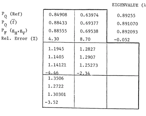
Results were obtained using options (a) and (b) for a small benchmark problem EPRI-9 (3x3x4). The magnitude of the errors in all cases are consistent with those to be expected using the FLARE model. Figures (2-1) and (2-2) show the results obtained using gh' gv-values and node-dependent g-values respectively. For illustrative purposes, these figures also include results using QUANDRY but with the face-dependent discontinuity factors replaced by their node-averaged values. Since averaging
discontinuity factors (or more precisely, the g-factors derived from the face-dependent discontinuity factors) is the only approximation made other than the axial averaging of the albedos, these should be much closer to the FLARE results, which is seen to be the case. It is to be noted that only a very small reduction in the relative errors of the eigenvalue A and the assembly and mid-plane nodal power densities is achieved when
node-dependent g-values are used. However, it was concluded that the small size of the core, with the majority of the nodes having external surfaces, did not make it a suitable test candidate for the FLARE model, with its inherent assumption that the kernel WPq is the same for all adjacent nodes.
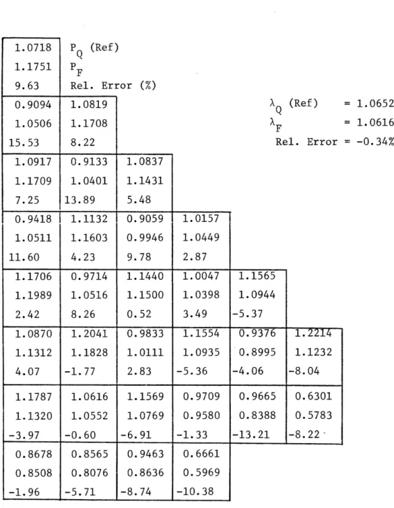
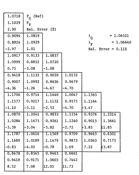
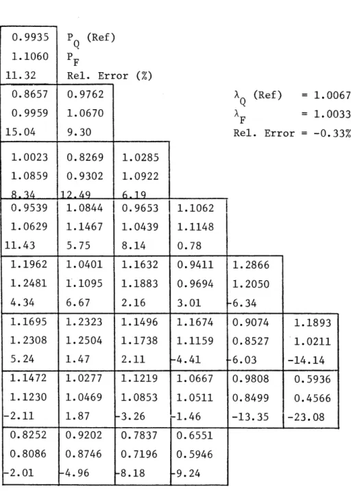
A more realistic test case is the SALEM-1 PWR (8x8x9). Results are shown in Figs. (2-3) and (2-4). It is immediately apparent that a very
dramatic improvement in the errors is obtained using node-dependent
g-values. For example, the relative error in the eigenvalue decreased from - 0.34 % to - 0.11 %, and the maximum errors in the assembly power
densities (in the interior of the core) from = 15 % to 6%.
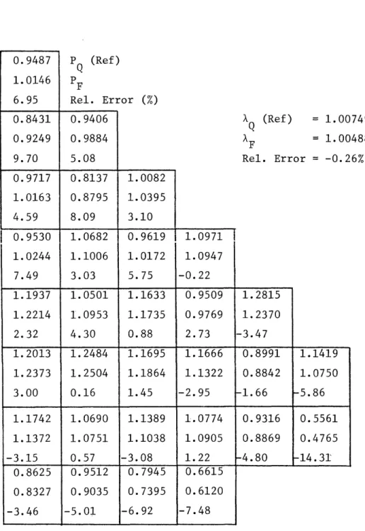
Depletion studies were carried out on ZION-2 (8x8xl). Results are shown in Figs. (2-5) - (2-10). As in the SALEM-1 case, there is a very significant reduction in the errors when node-dependent g-values are used, with the relative error in the eigenvalue decreasing from -0.26 % to
-0.02 % at B-O-L. Maximum errors in the interior of the core are also reduced from = 10 % to = 4%. Both options show a large increase in the respective errors at the first depletion (60 hours), but these continue to increase more gradually up to the final depletion step (7800 hours). This result suggests that it would be preferable to use the 60-hour (equilibrium xenon) case to find the node-averaged discontinuity factors, thence gp values.
EPRI-9: (3 x 3) x 4 ASSEMBLY POWER DENSITIES
EIGENVALUE (X) PF (gH'gV) Rel. Error (%) 0.84908 0.88433 0.88555 4.30 1.1945
1.1405
1.14121 -4.461.3506
1.2722
1.30301
-3.52
0.63974 0.69377 0.69538 8.701.2827
1.2907
1.25273-2.34
0.89255 0.891070 0.892093 -0.052NODAL POWER DENSITIES
(Ref) (f) (%) PF (gH'gV) Rel. Error
1.0656
1.1193
1.14203
7.17 1.5008 1.4359 1.47174 -1.94 .... _ _1.6981
1.6015
1.68040 -1.04Fig. (2-1). Assembly and Mid-plane Nodal Power Densities Using
(a) QUANDRY, (b) QUANDRY with fP, (c) FLARE-G with gH' gV-PQ PQ (Ref) (f) PQ PQ
0.80828
0.882120.89678
10.95 1.6293 1.6387 1.61556 -0.84 II I IEPRI-9: (3 x 3) x 4 ASSEMBLY POWER DENSITIES
EIGENVALUE (A) Rel. Error (%) 0.84908 0.88433 0.88996 4.81 1.1945 1.1405 1.14449 -4.19 1.3506 1.2722 1.27005 -5.96 0.63974 0.69377 0.68800 7.54 1.2827 1.2907 1.28507 0.18 0.892555 0.891070 0.892174 -0.043 PQ PQ (Ref) (f) PF (gp) Rel. Error (%)
NODAL POWER DENSITIES
1.0656 0.80828 1.1193 0.88212 1.4697 0.87954 7.64 8.82 1.5008 1.6293 1.4359 1.6387 1.46645 1.66607 -2.29 2.26 1.6981 1.6015 1.63206 -3.89
Fig. (2-2). Assembly and Mid-plane Nodal Po er Densities Using PQ PQ PF (Ref) (f) (gp) | R = | _ I
PQ (Ref) PF Rel. Error (%) 1.0819 1.1708 8.22 0.9133 1.0401 13.89 1.1132 1.1603 4.23 0.9714 1.0516 8.26 1.2041 1.1828 -1.77 1.0616 1.0552 -0.60 0.8565 0.8076 -5.71 XQ (Ref) = 1.06521 F = 1.06161 Rel. Error = -0.34% 1.0837 1.1431 5.48 0.9059 0.9946 9.78 1.1440 1.1500 0.52 0.9833 1.0111 2.83 1.1569 1.0769 -6.91 0.9463 0.8636 -8.74 1.0157 1.0449 2.87 1.0047 1.0398 3.49 1.1554 1.0935 -5.36 0.9709 0.9580 -1.33 0.6661 0.5969 -10.38 1.1565 1.0944 -5.37 0.9376 0.8995 -4.06 0.9665 0.8388 -13.21 1.2214 1.1232 -8.04 0.6301 0.5783 -8.22'
Fig. (2-3). Assembly Power Densities for SALEM-1
Using (a) QUANDRY, (b) FLARE-G with gH' gv. 1.0718 1.1751 9.63 0.9094 1.0506 15.53 1.0917 1.1709 7.25 0.9418 1.0511 11.60 1.1706 1.1989 2.42 1.0870 1.1312 4.07 1.1787 1.1320 -3.97 0.8678 0.8508 -1.96 S-| - | - -.
PQ (Ref) PF Rel. Error (%) 1.0819 1.0929 1.01 0.9133 0.8852 -3.08 1.1132 1.0992 -1.26 0.9714 0.9217 -5.11 1.2041 1.1675 -3.04 1.0616 1.0189 -4.02 0.8565 0.9171 7.08 XQ = 1.06521 xF = 1.06640 Rel. Error = 0.11% 1.0837 1.0720 -1.08 0.9059 0.8636 -4.67 1.1440 1.1152 -2.52 0.9833 0.9261 -5.82 1.1569 1.1479 -0.78 0.9463 1.0603 12.05 1.0152 0.9679 -4.70 1.0047 0.9575 -4.70 1.1554 1.1240 -2.72 0.9709 0.9873 1.69 0.6661 0.7442 11.73 1.1565 1.1164 -3.47 0.9376 0.9015 -3.85 0.9665 1.0363 7.22 1.2214 1.3661 11.85 0.6301 0.7175 L3.87
Fig. (2-4). Assembly Power Densities for SALEM-1
Using (a) QUANDRY, (b) FLARE-G with g - Values. P. 1.0718 1.1029 2.90 0.9094 0.8824 -2.97 1.0917 1.0999 0.75 0.9418 0.9007 -4.36 1.1706 1.1577 -1.10 1.0870 1.0284 -5.39 1.1787 1.1689 -0.83 0.8678 0.9418 8.52 __ I I
PQ (Ref) PF Rel. Error (%) 0.9406 0.9884 5.08 0.8137 0.8795 8.09 1.0682 1.1006 3.03 1.0501 1.0953 4.30 1.2484 1.2504 0.16 1.0690 1.0751 0.57 0.9512 0.9035 -5.01 x (Ref) = 1.00749 tF = 1.00488 Rel. Error = -0.26% 1.0082 1.0395 3.10 0.9619 1.0172 5.75 1.1633 1.1735 0.88 1.1695 1.1864 1.45 1.1389 1.1038 -3.08 0.7945 0.7395 -6.92 1.0971 1.0947 -0.22 0.9509 0.9769 2.73 1.1666 1.1322 -2.95 1.0774 1.0905 1.22 0.6615 0.6120 -7.48 1.2815 1.2370 -3.47 0.8991 0.8842 -1.66 0.9316 0.8869 -4.80 1.1419 1.0750 -5.86 0.5561 0.4765 -14.31
Fig. (2-5). Nodal Power Densities for Zion-2 at B-O-L Using (a) QUANDRY, (b) FLARE-G with gH' gV
41 0.9487 1.0146 6.95 0.8431 0.9249 9.70 0.9717 1.0163 4.59 0.9530 1.0244 7.49 1.1937 1.2214 2.32 1. 2013 1.2373 3.00 1.1742 1.1372 -3.15 0.8625 0.8327 -3.46
PQ (Ref) PF Rel. Error (%) 0.9762 1.0670 9.30 0.8269 0.9302 1 9AQ 1.0844 1.1467 5.75 1.0401 1.1095 6.67 1.2323 1.2504 1.47 1.0277 1.0469 1.87 0.9202 0.8746 -4.96 1.0285 1.0922 19 0.9653 1.0439 8.14 1.1632 1.1883 2.16 1.1496 1.1738 2.11 1.1219 1.0853 -3.26 0.7837 0.7196 -8.18 AQ (Ref) = 1.00672 AF = 1.00339 Rel. Error = -0.33% 1.1062 1.1148 0.78 0.9411 0.9694 3.01 1.1674 1.1159 -4.41 1.0667 1.0511 -1.46 0.6551 0.5946 -9.24 1.2866 1.2050 -6.34 0.9074 0.8527 -6.03 0.9808 0.8499 -13.35 1.1893 1.0211 -14.14 0.5936 0.4566 -23.08
Fig. (2-6). Nodal Power Densities for Zion-2 at 60 Hrs. Using (a) QUANDRY, (b) FLARE-G with gH' gV' 0.9935 1.1060 11.32 0.8657 0.9959 15.04 1.0023 1.0859 8R -0.9539 1.0629 11.43 1.1962 1.2481 4.34 1.1695 1.2308 5.24 1.1472 1.1230 -2.11 0.8252 0.8086 -2.01 I I I I m 7__ - . f U·ll
PQ (Ref) PF Rel. Error (%) 1.2086 1.3486 11.58 1.1443 1.2977 13.41 1.1804 1.2732 7.86 1.1621 1.2365 6.40 1.0968 1.1130 1.48 0.9795 0.9918 1.26 0.7474 0.7137 -4.51 AQ(Ref) = 1.01314 AF = 1.00973 Rel. Error = -0.34% 1.1847 1.2920 9.06 1.1826 1.2801 8.24 1.1436 1.1747 2.72 1.1331 1.1289 -0.37 0.9521 0.9201 -3.36 0.6583 0.5795 -11.97 1.156b 1.1876 2.59 1.0792 1.0757 -0.32 1.0603 1.0000 -5.69 0.9582 0.9122 -4.80 0.5624 0.4931 -12.32 1.1790 1.0752 -8.80 0.9444 0.8143 -13.78 0.8304 0.7046 -15.15 0.9885 0.8136 -17.69 0.5143 0.3633 -29.36
Fig. (2-7). Nodal Power Densities for Zion-2 at 7800 Hrs. using (a) QUANDRY, (b) FLARE-G with gH' gV
43 1.2336 1.3790 11.79 1. 2193 1.4027 15.04 1.2002 1.3281 10.66 1.1859 1.3194 11.26 1.1576 1.2138 4.85 1.1440 1.1694 2.22 0.9724 0.9615 -1.12 0.6852 0.6495 -5.21 _ ____ ____ ]l F S_ _ ____ -- -- ~ -. __ .
PQ (Ref) PF Rel. Error (%) 0.9406 0.9287 -1.27 0.8137 0.7825 -3.83 1.0682 1.0403 -2.61 1.0501 1'.0093 -3.89 1.2484 1.2198 -2.29 1.0690 1.0571 -1.11 U. 9l12 1.0389 9.22 (Ref) = 1.00749 = 1.00732 F Rel. Error = -0.02% 1.0082 0.9768 -3.11 0.9619 0.9333 -2.97 1.1633 1.1252 -3.28 1.1695 1.1454 -2.06 1.1389 1.1396 0.06 U. 43 0.8479 6.72 1.0971 1.0500 -4.29 0.9509 0.9123 -4.06 1. 1666 1.1370 -2.54 1.0774 1.1398 5.79 U. bbJ5
0.7225
9.22 1.2815 1.2585 -1.79 0.8991 0.8907 -0.93 0.9316 0.99406.70
1.1419 1.1872 3.97 0.5561 0.5944 6.89 ....Fig. (2-8). Nodal Power Densities for Zion-2 at B-O-L
Using (a) QUANDRY, (b) FLARE-G with g - Values. P 44 0.9487 0.9620 1.40 0.8431 0.8278 -1.81 0.9717 0.9610 -1.10 0.9530 0.9276 -2.67 1.1937 1.1721 -1.81 1.2013 1.1757 -2.13 1.1742 1.1670 -0.61 U. b2) 0.9178 6.41 -- -s -- w
-PQ (Ref) PF Rel. Error (%) 0.9762 1. 0211 4.60 0.8269 0.8381 1.35 1.0844 1.0993 1.37 1.0401 1.0273 -1.23 1.2323 1.2270 -0.43 1.0277 1.0236 -0.40 0.9202 0.9962 8.26 xQ(Ref) = 1.00672 IF = 1.00580 Rel. Error = -0.09% 1.0285 1.0421 1.32 0.9653 0.9653 0.00 1.1632 1.1491 -1.21 1.1496 1.1324 -1.50 1.1219 1.1224 0.04 0.7837 0.8194 4.56 1.1062 1.0799 -2.38 0.9411 0.9066 -3.67 1.1674 1.1233 -3.78 1.0667 1.0887 2.06 0.6551 0.6997 6.81 1.2866 1.2213 -5.08 0.9074 0.8537 -5.92 0.9808 0.9433 -3.82 1.1893 1.1126 -6.45 0.5936 0.5664 -4.58
Fig. (2-9). Nodal Power Densities for Zion-2 at 60 Hrs. Using (a) QUANDRY, (b) FLARE-G with gp- Values.
45 0.9935 1.0695 7.65 0.8657 0. 9045 4.48 1.0023 1.0451 4.27 0.9539 0.9720
1.90
1.1962 1.2104 1.19 1.1695 1.1706 0.09 1.1472 1.1558 0.75 0.8252 0.8838 7.10 -l .. . ...PQ (Ref) PF Rel. (Error (%) 1.2086 1.2120 0.28 1.1443 1.2470 8.97 1.1804 1.1617 -1.58 1.1621 1.2637 8.74 1.0968 1.0611 -3.25 0.9795 1.0715 9.39 0.7474 0.7986 6.85 XQ(Ref) = 1.01314 tF = 1.01069 Rel. Error = -0.24% 1.1847 1.1620 -1.92 1.1826 1.2765 7.94 1.1436 1.0853 -5.10 1.1331 1.1669 2.98 0.9521 0.9332 -1.99 0.6583 0.6761 2.70 1.1576 1.0848 -6.29 1.0792 1.0772 -0.19 1.0603 0.9593 -9.53 0.9582 0.9858 2.88 0.5624 0.5938 5.58 1.1790 0.9877 -16.23 0. 9444 0.8556 -9.40 0.8304 0.7394 -10.96 0.9885 0.8007 -19.00 0.5143 0.4362 -15.19
Fig. (2-10). Nodal Power Densities for Zion-2 at 7800 Hrs. Using (a) QUANDRY, (b) FLARE-G with gp- Values.
46 1.2336 1.2540 1.65 1.2193 1.3609 11.61 1.2002 1.2025 0.19 1.1859 1.3145 10.84 1.1576 1.1337 -2.06 1.1440 1.2039 5.24 0.9724 0.9725 0.01 0.6852 0.7239 5.65 _ - --. . ._ .. _ -- . _ ...
2.4 PRESTO MODEL: REDUCTION OF QUANDRY-CMFD EQUATIONS
We first approximate the six discontinuity factors for each node, fiJk (u = xy,z) by ,j
gu. g , so that the QUANDRY-CMFD equations
(2.26) become,
ki+l, jk
kijk
-1
- 2k g +
I[
i+,jk i+l,ljk i+,jk ijk ijkDi+l,jk Dijk g g g g g g - i-l,jk + 2k g Di-l,jk g - i,j+l,k - 2k g
D
i,j+l ,k
g kijk-1
+ g Dij k giijk ijk i-l,jk i-l,jk
g g g g
pijk
--1
FDijk i,j+l,k i,j+l,k ijk iik 1
Dijk g - i,j-1,k + 2k g Di,j -1,k g
fijk
-1
+
Dijk gijk ijk i,j-l,k i,j-l,k
g g g g
Lij,k+l kijk - -1
Dij9k~ ij 9ij,k+l [ ij,k+l ijk ijk
ij,k+l ijk g g
D
i j k
D
g
+ 2 - i jk jk ijk ij,k-1 ij,k-1 Dij,k- Dijk g g G + h2k Ziij k i,j,k i h2k g ' g L g '=1
[-
Xgfi,k
+ Eij,k] i,j,k
A XEfg,)L~~~~g 2 h2
k
g
We then define the following parameters:
g*i,j,k ij,k ijk
g g g
D
*i,jk
g Di,j,k_g
fi,j,k g zi ,j,k 9g ijk g so that - 2k ki+l,jk g Di+l,jk g ijk + g Dijk g -1i+l,jk i+l,jk
g g - ijk k g 9-
- 2k [ - D*i+l,j,k g = -2k -1 + 1 1 [ *i+l,jk D*i,j,k J g D*i+l,j,k D*i,j,k g g D*i+l,j,k + D*i,j,k g g *ij,k ]E
*i+l,j ,k *i,j,k 9 9~cg 'and similarly for the other terms in Eq. (2.48). Hence the QUANDRY-CMFD equations are reduced to:
(2.49)
4 - 2k
qh
=l
D*P D*q * [g g g q- WgPDP +
D
q
g g G 2 1 *p *p=h2k
-
XgZfg,
+
gg
g =1 2 D*P D*q 2kR g [ gq q =1 D* p + D* q v g g tg 6gg, ] gThe fast group equation (g = 1) is given (neglecting the subscript)
by :
4
D
Dq
D*
q
-
2k
[*q - *P ]
2kR
-
[ *q
*p
]
1' D*Ph~~~~~~~~~~~
Dq+
q ql+ =lv
D +D*q (2.52)=h
2k [ 1 kp
-
1
z*p *
L
o
This equation has the same structure as the PRESTO equation (2.20), except that only ' p occur here, whereas the previous equation contains 'P and
p
'P In order to make the form of the two equations identical, we
-p rearrange the PRESTO equation by introducing the PRESTO expression for 'P
given by Eq. (2.14) into Eq. (2.20), which can finally be written as follows:
- P
]
4 Dp Dq 2 Dp Dq 2k 1 p q 0P 2kR [q ] - 2 2[ -- P [ q [q - ] P
q1
D
ph +
D
q=1
D
p+ D
q 1 p =h 2k k 1 - P (2.53) 1 +-where h2k - 1 ] P (2.54) P 2kDP 3a + (1 - a) (R + 2)Except that D appears rather than D , and center-point fluxes qp are replaced by fictitious nodal fluxes P , equation (2.53) is now identical to the reduced QUANDRY-CMFD equation (2.52), provided that we also interpret ZP / (1+7P) as Z* P = / P . This implies that
1 + P = fP
so that an expression for "a" may be determined from Eq. (2.54). It is given by:
h2 1 k 1] Zp - 4 DP (fP - 1) (R + 2)
aP = (2.55)
h2 [ 1 kP - 1 ] P + 4 D (P - 1) (1 - R) A
For R = 1, i.e. h = k:
ap =1 - 12 D - ( 2.56)
h2 1 kP - 1] Zp
SOLUTION OF PRESTO EQUATIONS
The PRESTO code is proprietary material, and hence is not available to the general public. Therefore, in order to test the above scheme, it is necessary to solve the PRESTO equations using some alternative code, which is available. Since QUANDRY was developed at MIT and is easily modified for the present purpose, it was decided that it could be used to solve the PRESTO equations. This is not completely satisfactory, and in fact appears a circular procedure, since QUANDRY is first used in order to determine the adjustable parameter a ( or aP). We take the view that the two stages are completely independent. In the first stage, by running QUANDRY in the normal manner, the parameters obtained, i.e. A, fP,... etc. permit ap
to be calculated, and hence a = a . Having determined "a", the PRESTO equations can now be solved by any suitable method, including of course PRESTO itself. It seems, however, that the different solutions thus
obtained will not be identical, since different procedures, including the specification of boundary conditions are involved, and may not be exactly duplicated in each case. For example, it may be noted that an iterative scheme is used in PRESTO to solve the fast-group equation, which is written in an entirely equivalent form for the case h = k,
Dp Dq 2k [ q ~P] g=l DP + Dq P p P 1_3[_f l f2 21 p i P -p (2.57) 3 1 CP P P Ip 1 1 2
where Fp = / P ) P being the actual nodal-averaged thermal
Wh2 ~2(asy) 2
flux, and P2(asy) the asymptotic value given by
OP2(asy) = [ P / ] P . F is initially set equal to unity, and the equation solved to yield 9P , so that -P can be determined. It is
1 2(asy)
then assumed that the asymptotic values for the point fluxes (p2 hold at the centers of the nodes,
p 21-p
2 p 1 (2.58)
2
so that the thermal node-averaged flux may be reconstructed in a way similar to that used for the fast group,
- a2 - V Pq (2.59)
02 a2 2 6 £
q=l
-
-FP = / 2(asy) is then updated, so that the fast group can be solved again to obtain an improved value for P , and the iterative process repeated until convergence is achieved. A further approximation which we have neglected was introduced in PRESTO to reduce the data storage
requirements.
In our case, however, the reference solution is already available, since it is necessary to determine the a -values . Thus we can use the
p
known ratio of the thermal to fast flux to calculate P directly (i.e. without iteration), and hence P and the nodal powers. In
particular, we note that when a = 1, the nodal volume-averaged fluxes (p and the centre-point fluxes P are identical, and equations (2.52) and
(2.53) are the same except that the "starred" cross-sections (D*p, P...) given by Eq. (2.49) appear in place of the physical cross-sections
(D, P,...). Hence, one approach to solving the PRESTO equations on QUANDRY is to set a = 1 and replace the physical cross-sections by their starred equivalents. While the flux solution obtained is a "fictitious nodal volume-averaged flux" 'P , the reaction rates are unchanged, so that the nodal powers have their true physical values, since
[
fl 1 f2 2 fl L P1 + f2 p p] __ [ P + f2 P U 2 2' 1 2 - f P + f2p]
(2.60)fl 1
f22
One objection to this approach is that by setting a = 1, the
fundamental assumption in the PRESTO model given by equations (2.14) and (2.15), which distinguishes the MCMFD model from previous CMFD models has been circumvented. However, there does not seem to be any alternative given
the limitation of having to use QUANDRY to solve the PRESTO equations. In order to counter this objection, an investigation is currently being
undertaken to use the nodal code SIMULATE with the PRESTO option, so that a direct comparison can be made between the two methods.
PRESTO RESULTS
Results were obtained using QUANDRY for the SALEM-1 pressurized water reactor at B-O-L, and are shown in Figs. (2-11) and (2-12). Since
node-dependent discontinuity factors are used, this is equivalent to using PRESTO with node-dependent a -values . The relative error in the
p
eigenvalue is < 0.2 %, with maximum errors of < 10 % in the assembly and nodal power densities. Depletion studies are presently being carried out on ZION - 2.
CONCLUSIONS
Until further testing is complete, conclusions must be tentative.
However, at present, it appears that if node-dependent coupling coefficients and albedos are permitted for the FLARE and PRESTO models the accuracy is about that achieved when the usual trial-and-error procedure is used to find the adjustable parameters for the FLARE and SIMULATE models. There thus is no compelling reason to determine the FLARE and PRESTO parameters
PQ (Ref) Pp Rel. Error (%) 1.0819 1.1214 3.65 0.9133 0.9592 5.03 1.1132 1.1309 1.59 0.9714 0.9875 1.66 1.2041 1.1502 -4.48 1.0616 1.0194 -3.98 0.8565 0.8858 3.42 1.0837 1.1250 3.81 0.9059 0.9240 1.99 1.1440 1.1528 0.77
0.9833
0.9708 -1.26 1.1569 1.0932 -5.51 0.9463 0.9832 3.90 Q(Ref) = 1.06521 p = 1.06336 Rel. Error = -0.17% 1.0157 1.0173 0.16 1.0047 1.0097 0.50 1.1554 1.0874 -5.89 0.9709 0.9673 -0.38 0.6661 0.6777 1.75 1.1565 1.1411 -1.33 0.9376 0. 9119 -2.74 0.9665 0.9618 -0.49 1.2214 1.2724 4.18 0.6301 0.6603 4.79Fig. (2-11). Assembly Power Densities for SALEM-1 at B-O-L Using (a) QUANDRY, (b) PRESTO (QUANDRY).
55 -- 1 1.0718 1.1593 8.16 0.9094 0.9486 4.32 1.0917 1.1186 2.46 0.9418 0.9509 0.97 1.1706 1.1570 -1.16 1.0870 1.0540 -3.04 1.1787 1.1135 -5.53 0.8678 0.8740 0.71 _Il - .-_ _ .
PQ (Ref) Pp Rel. Error (%) 1.6312 1.7197 5.43 1.3768 1.4699 6.76 1.6782 1.7340 3.32 1.4642 1.5116 3.24 1.8150 1.7593 -3.07 1.5997 1.5553 -2.78 1.2905 1.3430 4.07 1.6337 1.7249 5.58 1.3656 1.4133 3.49 1.7245 1.7650 2.35 1.4819 1.4827 0.05 1.7434 1.6666 -4.41 1.4257 1.4900 4.51
Fig. (2-12). Mid-plane Nodal Power Densities for SALEM-1 at B-0-L Using (a) QUANDRY, (b) PRESTO (QUANDRY).
1.6160 1.7671 9.35 1.3709 1.4522 5.93 1.6460 1.7169 4.31 1.4197 1.4569 2.62 1.7646 1.7742 0.54 1.6384 1.6115 -1.64 1.7765 1.7016 -4.22 1.3076 1.3299 1.71 1.5310 1.5496 1.21 1.5143 1.5414 1.79 1.7414 1.6591 -4.73 1.4630 1.4696 0.45 1.0036 1.0054 0.18 1.7431 1.7428 -0.02 1.4129 1.3876 -1.79 1.4562 1.4583 0.14 1.8402 1.9317 4.97 0.9493 1.0014 5.49 ·,,,, -.. _ . .
in this alternative manner, even though it is more systematic than the trial-and-error procedures in current use. In our opinion, computing
effort required to implement the automatic scheme would be far better spent on a production version of QUANDRY.
3. DEVELOPMENT OF A MORE EFFICIENT FLUX RECONSTRUCTION METHOD FOR BWRs - A. Z. TANKER
Although discontinuity factors found from assembly calculations lead to accurate predictions of kf f and average nodal powers for BWRs,
reconstructing detailed pin power shapes has required the use of response matrices or extended assembly calculations.
During the past year, computer codes have been constructed to carry out the reconstruction using a fine-mesh, beginning-of-life, quarter-core solution. A small, "benchmark," test problem has been created and a one-cycle depletion carried out. We are now applying our new
flux-reconstruction method to this reference case and expect to complete the testing during the coming year.
4. Development of Methods to Analyze Transients - Antonio Dias
We had hoped, during the past year, to begin an investigation of the use of "supernodes" (of size - 40 x 40 x 60 cm ) for the analysis of reactor transients. However, the static application of this technique
(supported by other funds) ran into a technical difficulty which we are only now beginning to understand. That understanding does, however, indi-cate that applying the method to transient analysis is still an attractive possibility. We hope to explore it during the coming year.
For many situations, however, transients that occur in a reactor have a one-dimensional character such that the perturbations are uniform in radial planes but quite non-uniform in the axial direction. Examples of such transients are a rod bank withdrawal, a loss of flow accident and a turbine trip accident. The assumption that the x,y shape of the neutron distribution is unperturbed during the transient is then more plausible than that required for the point kinetics approach. Introducing this idea into a nodal method should result in a theory that allows the simulation of certain transients with better precision than if point kinetics were used, but with greater speed than if a full 3-D nodal approach were considered.
A one-dimensional model is available on option in the RETRAN code. However, it appears to ignore radial leakage effects. In the work described below, we have used a variational principle to derive one-dimensional,
G-group transient equations directly from the QUANDRY nodal equations. This procedure has the advantage of treating radial leakage effects in a
theoreti-cally consistent way. In addition, the parameters needed for the one-dimensional equations can be computed directly from a static, three-dimensional, beginning-of-transient QUANDRY solution. Of even greater
one-dimensional equations by direct comparison with three-dimensional QUANDRY results based on consistent time-dependent nodal cross sections.
4.1 Derivation of the Theory
The QUANDRY nodal represented as: ()
[v-l]
[][o] [o] [o ]
[o]
..[o]
[o]
[]
[o] [o] ...
[o]
[]
o] [o] []
[]
..-[o]
[o] [o] [o] [o] ...[o]
[o]
[a]
[o]
[o]
...
[o]
[L]
[o]
[o]
[o]
...equations for a 3-D transient problem can be
[o]
[o]
[o]
lo]
[o][o]
d dt [(t)] [Lx(t)] [L (t) [L (t)] [CD (t) ] D-[M (t)]-[T (t)] [Fx (t)] [Fy (t)] [Fz (t)] [M1 (t) [MD (t)]-hhk[I]
y z-h
x zh
[I]
-hihJ[I]
x yl[I]
-[I]
1
i[Gy
(t) x hi[Gz(t )]x
[o]
[o] 1 hj[Gx( t)] y-I]
1 -j[GZ( t)]y
[o]
[o] 1 k[G (t).] [o] z hk[G (t)] hk y z -[I] [o][o]
[o] -1[I][o]
[o]
(4.1)D]
.* [o]*·
[o]
·. · [o]D[]
[(t)]
[Lx(t)] [Ly (t)] [i z(t)] [C (t) ] [CD (t)] *-where:
[¢(t)] - a column vector of length G x (I x J x K) (-N) containing the node averaged fluxes (ordered first by group, then x-direction, then y-direction, and finally z-direction)
[L (t)] a column vector of length N containing the u-directed net leakages for each node . u = x, y, or z
[Cd(t)] a column vector of length N containing, for the d-precursor family, the elements of Vijk[Xd]Cd (t)
ijk
[V-1] a block diagonal matrix of order N x N containing the elements of
Vijk[V]-[M (t)] - a block diagonal matrix of order N x N containing the elements of (l-B)Vijk[Xp] [f (t)]T
jk
[zT(t)]
I
a block diagonal matrix of order N x N containing the elements of Vijk[zTi (t)] with [ T (t)] equal to the G x G matrixijk ijk
{6 Z(ijk) - (ijk)} gg' tg gg'
[F (t)] _ a block tridiagonal matrix of order N x N containing the elements
u
of [Fz (t)] specifying leakage in the u-direction u mn
[G(t)] - a block pentadiagonal matrix of order N x N containing the elements of [GU (t)] specifying leakage transverse to the u-direction
Zmn
[Md(t)] - a block diagonal matrix of order N x N containing, for the d-precursor family, the elements of dVijk[ d] [vZf (t)]T
Detailed expressions for the elements of the vectors and matrices cited above are given in Reference (8).
The systematic derivation of equations presented in this work is due to the application of a synthesis method based on a variational principal (3),(9). In order to implement this approach, it is necessary to construct a
func-tional that is made stationary by the solutions of the QUANDRY equations (eq. 4.1).
The functional in question is defined for a set of functions:
{[u(t)], [vx(t)], [ (t)], [cl(t)], ct .. , [cD(t)], [u*(t)],
x y z 1 D
[v (t)], [(t)], [z(t)], [ct)] , [cd(t)]}
these functions are to be continuous in time within the time interval (t , t f), during which the simulation takes place.
Each of these functions is actually a column vector of length GI-J-K The expression for the functional is:
F([u], I[v] [v] rIv [cl] IC . , [c], [u ], [v*], [v*], [v], [c], . ,
tf
[C*]) =
fdt
[ [u ] [v ] v] cl] . . * x toMp]-[T]-[V-1] dt -hyh[I] IFx] [Fy] [Fz] [M1] [M1 ] -[I] i[Gy]
h
i
x - [G ]hz
x.[o]
[o]
-hihk[I] 1 [G y -[I] 1 [G ]h
j
y
[o]
[o]
-hh] [I] I11]
xy
1
-k[G
x ] hk x z ! [Gy] hk y z -[I][o],
[o] d dt 1where dt is considered as an operator.
In order to keep notation simpler, the time-dependence is not shown. Such suppression will be adopted for all equations which follow.
For the application of the synthesis method, the following set of trial functions are defined:
[u] = [] T] Ivx] = [:] [x]