Segmentation of retinal vessels in adaptive optics images for assessment of vasculitis

HAL Id: hal-01567288

https://hal.archives-ouvertes.fr/hal-01567288

Submitted on 22 Jul 2017

HAL is a multi-disciplinary open access

archive for the deposit and dissemination of

sci-entific research documents, whether they are

pub-lished or not. The documents may come from

teaching and research institutions in France or

abroad, or from public or private research centers.

L’archive ouverte pluridisciplinaire HAL, est

destinée au dépôt et à la diffusion de documents

scientifiques de niveau recherche, publiés ou non,

émanant des établissements d’enseignement et de

recherche français ou étrangers, des laboratoires

publics ou privés.

Segmentation of retinal vessels in adaptive optics images

for assessment of vasculitis

Marthe Lagarrigue-Charbonnier, Florence Rossant, Isabelle Bloch,

Marie-Hélène Errera, Michel Paques

To cite this version:

Marthe Lagarrigue-Charbonnier, Florence Rossant, Isabelle Bloch, Marie-Hélène Errera, Michel

Paques. Segmentation of retinal vessels in adaptive optics images for assessment of vasculitis. IEEE

6th International Conference on Image Processing Theory, Tools and Applications (IPTA’16), Dec

2016, OULU, Finland. pp.1 - 6, �10.1109/IPTA.2016.7821037�. �hal-01567288�

Segmentation of retinal vessels in adaptive optics images for assessment of vasculitis

Marthe Lagarrigue-Charbonnier

1

_{, Florence Rossant}

2

_{, Isabelle Bloch}

3

_,

Marie-Hélène Errera

4

_{, Michel Paques}

4

1_{Université Pierre et Marie Curie (UPMC), Paris, France}

e-mail: marthe.charbonnier@upmc.fr

2_{Institut Supérieur d’Électronique de Paris (ISEP), France}

e-mail: florence.rossant@isep.fr

3 _{CNRS, LTCI, Télécom ParisTech, Université Paris-Saclay, Paris, France}

e-mail: isabelle.bloch@telecom-paristech.fr

3 _{Clinical Investigation Center 1423, Centre Hospitalier National des Quinze-Vingt, Paris, France}

e-mail: errera.mhelene@gmail.com, michel.paques@gmail.com

Abstract—In this paper we propose a new method for

segmenting retinal vessels in adaptive optics images. This method is particularly dedicated for segmenting vessels with significant morphological alterations due to vasculitis, but it is also accurate for vessels with moderate or without alteration. It relies on a pre-segmentation step which is crucial for the robustness and accuracy of the results. This step is based on a specific morphological processing of isolines of the original image: they constitute of good basis for the segmentation because they are disposed along the wall borders of the vessels. Regularization is then performed using active contour model embedding a parallelism constraint. This novel model allows precise segmenting inner and outer walls of the vessel. In particular it is more accurate in the case of vasculitis than the existing methods. This is the only method that allows quantification. The results and the runtime make it suitable for clinical use.

Keywords— Parallel snakes, isolines, retinal vessels segmentation, vasculitis, adaptive optics imaging.

I. INTRODUCTION

In this paper, we address the problem of segmentation of retinal vessels in difficult pathological cases (namely vasculitis) from recently developed adaptive optics imaging [1]. Retinal vasculitis is an inflammation of retinal vessels that may occur in the course of various inflammatory diseases, either as an isolated or systemic disease. It affects veins more frequently than arteries. Clinically, retinal vasculitis appears as a vascular sheathing more or less visible on retinal photography. Until recently, there has not been any quantitative study of retinal vasculitis. As recently reported, flood illumination adaptive optics (FIAO) imaging allows for sensitive detection of retinal vasculitis [2]. FIAO is a recent technology that enables the visualization of retinal microstructures such as photoreceptors [3] and arterial walls [4], noninvasively [5]. The resolution of the Rtx1 camera [6] used in our study is about 1.6µm/pixel. To be processed, the raw images are averaged as detailed in [7]. With FIAO, vascular sheathing appears as fusiform or linear opacities up to 50µm wide, on both sides of vessels, often co-localized with focal vascular narrowing. The width of the perivascular opacification follows the clinical course of the disease, making an interesting biomarker. Such opacification most likely corresponds to the infiltration of the inflammation cells when comparing to previous histopathology findings of retinal vasculitis. Both vasculitis symptoms are illustrated in Fig. 1. The segmentation of artery walls is especially difficult, even in case of healthy patients, because of several factors: (i) high textured background, (ii) significant intensity variation along the lumens (Fig. 1) even if they

are globally dark, (iii) local discontinuities or poor contrast of the axial reflection, (iv) low-contrast of the outer borders of the walls, (v) local blurring of the segments due to the geometry of the retina, (vi) local deformations along vessels in case of pathologies, (vii) high variability in the images.

a) 766 × 667 pixels b) 383 × 333 pixels

c) 333 × 200 pixels

Fig. 1. a) Image of healthy retinal artery and vein acquired with the Rtx1 camera [6] [7]; b) Detailed view of a healthy artery; c) Image of

artery with vasculitis symptoms. Image resolution: 1.6 µm/pixel. In our previous work, the segmentation of retinal vessels in Adaptive Optics images (FIAO) focused on the segmentation of arteries in healthy subjects and pathological subjects [8] [9] [10], and was based on two main steps: (i) a pre-segmentation step to initialize the four curves that delineate the parietal wall; (ii) the application of a new parametric snake algorithm integrating structural a priori information, such as the approximate parallelism of the interfaces and/or the approximate symmetry of the parietal wall with respect to the axial reflection. We proposed two models named respectively “parallel snakes” (PS) [8] [9] and “coupled parallel snakes” (CPS) [9]. Both are derived from the classical snakes of [11] but include additional terms in the energy functional in order to integrate structural information and thus gain in robustness and accuracy.

The pathologies we have addressed up to now (named pathological cases of Type 1 in the following) show moderate alteration of vessel morphology and the performances evaluated on the database were good: the automatic segmentations were close to those made by medical experts and the derived measures were in the range of those obtained by the experts, given the intra- and inter-expert variability [8] [9] [10]. However we observed that these

Axial reflection Arterial wall (Parietal structure) Lumen (Blood column) VEIN ARTERY Perivascular opacification

methods fail in case of diseases that alter strongly vessel morphology, as vasculitis. To the best of our knowledge, there are no other methods which address this problem in such images, due to their novelty.

In this paper, we propose a new pre-segmentation method that is more robust and accurate. This new pre-segmentation step is followed by the application of the coupled parallel snakes (CPS), leading to good performances for heathy cases, as well as difficult pathological cases, including vasculitis. The runtime is dramatically reduced, which is very important when processing large databases for clinical studies. In Section II, we briefly remind the approach of [8] [9] [10], and we show its limitations in vasculitis cases. In Section III we present the new method for the pre-segmentation step. Experiments are presented in Section IV. We show that the obtained accuracy on our previous databases (heathy cases and pathological cases of Type 1) is maintained while the performances on the vasculitis database are much higher.

II. SEGMENTATIONOF VESSELS WALLS AND LIMITS

The automatic pre-segmentation described in [8] [9] [10] is based on the detection of the axial reflection of the vessel branches followed by a tracking procedure to initialize the four curves that delineate approximatively the parietal wall, on both sides. Let us denote by V(s)=(x(s),y(s))T _{the curve representing the axial reflection}

(reference line), parameterized by s, and n

 

s the vector normal to this reference curve. In the pre-segmentation step, the four curves

Vi(s), i=1,…,4 are defined in Equations (1) by their local distance,

bint_{(s) or b}ext_{(s), to V(s):}                                                 s n s b s V s V s n s b s V s V s n s b s V s V s n s b s V s V s ext ext     4 3 int 2 int 1 , (1)

with bext_{(s)- b}int_{(s)>0, s.}

The formulation in (1) imposes a strict symmetry of the parietal structures with respect to V(s). The search for the starting point of the tracking procedure as well as the tracking itself are based on the optimization of a cost function including gradient information, regularity constraints and structural constraints (via the definition of the curves) (see [10] and [12] for more details).

Then the CPS active contour model [9] is applied to more accurately position the curves found by the pre-segmentation. In this step, the symmetry imposed in (1) is relaxed and the four curves are defined, as illustrated, in Fig. 2, by:

                                                             s b s b s b s b s n s b s V s V s n s b s V s V s n s b s V s V s n s b s V s V s 2 4 , 1 3 4 4 3 3 2 2 1 1 , ,     (2)

Fig. 2. Parametric representation of the model proposed in [9] [10]. Thus, the inner (respectively outer) curves do not have to lie at the same distance to the reference line; additionally, the wall thickness has not to be constant and can be different from one side to the other. However, we keep some interdependence between the four curves in the CPS model, defined by the following energy functional:







 













2 4 2 4





1 4 1 4



4 , 2 4 1 3 1 3 1 3 , 1 Im 4 1 4 1 ,..., , ,..., , , , , , , , ,..., , ,..., b b V V T b b V V S b b V V S b V R V E b b V V E k k k         



 where

1. EIm(Vk) is a classical image energy term based on gradient

information [11] [13],

2. R(V,bk) imposes an approximate parallelism between each

curve and the center line, by controlling the evolution of bk:







_

1



 



0 2 ' ,b b s ds V R k k ,

3. S(Vi,Vj,bi,bj) controls the variation of the wall thicknesses

with respect to the initial estimate,

4. T(V1,…V4,b1,…b4) controls the difference of wall thickness

between both sides:



V V b b





b

   

s b s b

 

s b

 

s



ds T 



1    0 2 2 4 1 3 4 1 4 1,..., , ,..., .

The interdependence expressed in R and T is useful to gain in robustness with respect to noise and lack of contrast. The importance of each term is weighted by a scalar (φ, ψ1,3, ψ2,4 and λ). Setting

ψ1,3=ψ2,4=0 and λ=0 leads to the PS model, where the four curves

evolve independently, the only implicit interdependence being their approximate parallelism with respect to V(s).

As explained in [8] [9] [10], accurate results are obtained for healthy arteries or arteries suffering of pathologies that do not strongly affect their morphology. Otherwise, the symmetry constraints imposed in the tracking process are too strong to deal with sharp or asymmetric deformation of the inner or outer borders. Moreover, tracking procedures are applied locally and lack robustness when analyzing difficult images. Fig. 3 shows the pre-segmentation and final pre-segmentation obtained for a case of vasculitis. The pre-segmentation is rather far from the desired contour and the application of the coupled parallel snakes cannot correct this bad initialization. Considering the 20 images of our database of vasculitis, the algorithm completely fails for two cases, provides inexact segmentation of the lumen for 11 cases, and can never find perivascular opacifications. These results show that our pre-segmentation algorithm has to be redesigned in order to deal with opacifications and focal vessel narrowings (i.e. sharp variation of lumen diameter), these two features being of high medical interest for the study of this new type of pathology. Note that the axial reflection is correctly detected. Hence this part of the method does not have to be modified.

Fig. 3. Vasculitis case and details (top); pre-segmentation (bottom-left) and segmentation (bottom-right) obtained by the method of [9].

The segmentation task must provide an accurate delineation of the vessel inner borders and an estimation of the outer side of the

Variation of the lumen diameter Perivascular

opacification. The main difficulties are related to the irregularities of the inner wall and the very low contrast at the outer sides of the opacification.

It is worth noting that the wall of veins is much thinner than the artery wall, and generally not visible in FIAO images, even in case of healthy patients. Also, the wall of arteries affected by vasculitis is generally not discernable either. So the outer border provided by our algorithm will be the outer side of the opacification in all cases of vasculitis presenting this feature, whether veins or arteries.

III.NOVEL PRE-SEGMENTATION ALGORITHM

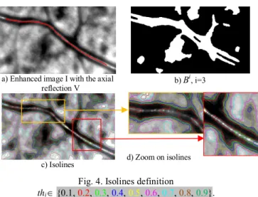
The original grayscale image is first enhanced by contrast stretching. The intensity values I(x,y) are normalized in the range [0,1]. We assume that the axial reflection V of every vessel branch is known (Fig. 4a), and obtained with the method described in [8]. Our new approach is based on the isolines of I to pre-segment the four searched borders.

A. Isoline extraction

Isolines are contours of holes and connected components of the binary image obtained after thresholding the grayscale image I at the levelsth_i

 

0,1.

a) Enhanced image I with the axial

reflection V b) B

i_{, i=3}

c) Isolines d) Zoom on isolines

Fig. 4. Isolines definition

thi {0.1, 0.2, 0.3, 0.4, 0.5, 0.6, 0.7, 0.8, 0.9}.

In our study, we assume that the overall image lighting is homogenous. We use 9 regularly spaced threshold values: thi=i/10,

i {1,…9}. The thresholding is followed by a morphological opening and a closing with a binary disk of radius 10 pixels, in order to remove the smallest components. We denote by Bi _{the binary image}

obtained for index i (Fig. 4b). Fig. 4c and Fig. 4d show the set of isolines found from the images Bi _{for the 9 thresholds. We observe}

that some of these isolines are located along the vessel and very close to the walls we want to localize. Thus, the pre-segmentation step amounts to selecting the most suitable contour points from the isolines. For that, we propose a three-step processing:

1. We pre-process each binary image Bi _{in order to get a}

single connected component Mi _{including the axial reflection and}

whose contours are close to the vessel borders (Section B).

2. We extract the relevant contour points from every mask

Mi_{, dealing with concavities and/or checking intensity properties. At}

the end, every point of the discretized central reflection line V has two correspondent contour points, one by side (Section C).

3. We select the index i that leads to the best pre-segmentation of the inner borders and the outer borders, by optimizing pixels intensity in regions or on curves defined by the selected relevant contour points (Section D and E).

B. Getting the masks M

i

Step 1 is achieved by intersecting the binary image Bi _{with a}

tubular region Tr_max centered on the axial reflection (Eq. 3) and

whose radius rmax140 pixels corresponds to the maximal size of retinal vessels (see Fig. 5a for i=2):







P I d PV r



T_r   / ,  , (3)

where d denotes the Euclidian distance.

We also detect the internal region of the vessel thanks to a classical region-growing algorithm applied to the morphological opening of the image I with a disk of radius r0. The purpose of the

opening is to remove the axial reflection (Fig. 5b). The radius r0 (Eq.

4) of the structuring element corresponds to the radius of the tubular region centered on V which minimizes the mean intensity in I:

  _{ }

 

_        



  r T y x r r y x I T Arg r , 75 , 0 0 , 1 min , (4)

where |T| denotes the cardinality of the set T.

The seed of the region growing algorithm is made of the points of

V. The resulting binary image is denoted by M0 _{(Fig. 5c). We select}

the relevant connected components of Bi _{∩ T}

rmax by performing a

reconstruction of M0 _{under the image B}i _{∩ T}

rmax. In this way, the

retained connected components are the ones that intersect the vessel. We finally fusion the resulting image with M0_{, providing (Fig. 5d)}

the image Mi_.

(a) Bi _{∩ T}

rmax (b) Image opening

(c) M0

(d) M2

Fig. 5. Definition the mask Mi _{for i=2.}

C. Selection of contour points from

Mi

Step 2 deals with potential concavities to select relevant points. Let us denote by V(s) the sampled reference line, where s=hk and h is the sampling interval, and n

 

s the vector normal to V at V(s). For every point V(s), we want now to define two corresponding points

Vji(s) on either side of the central reflection (j=1,2), as close as

possible to the inner vessel borders. As the contour of the mask Mi may exhibit irregularities and concavities, one has to select the suitable candidates.

Let us consider a specific point V(s) of the axial reflection. Candidate border points C are the contour points of Mi _{that are close to the}

straight line passing through V(s) and normal to V at V(s). They can be easily selected on both sides of V by calculating the determinant

   



CV s ,ns



det (almost 0) and the sign of the inner product

   

s ns

CV . . For each side j, we select as Vji(s) the candidate point

which is the closest to V(s). We finally check the orientation of the image gradient vector at this point, knowing that the internal part of the vessel is darker that the external part. In case of inconsistency,

Thus we get a unique pair (V1i(s), V2i(s)) of border points for each

V(s), and this for every mask Mi_.

D. Pre-segmentation of the inner borders of the walls

As the overall image illumination is homogenous, we can suppose that the intensity is rather stable along the two inner borders of the vessels. This is why we search for two sets of candidates Vji,

j=1,2, coming from the same level thi. We select the index i0 that

minimizes the mean intensity level of the pixels inside the region delimited by V1i and V2i. Fig. 6 illustrates the result found in the

example of Fig. 4a. In this case, i0 = 2. Most of the points are

actually on the inner borders, and the other ones will be easily corrected thanks to the image and regularization forces of the CPS active contour model, providing the inner borders i0

j

V , j=1,2.

Fig. 6. Pre-segmentation of inner walls and zoom.

E. Pre-segmentation of the outer borders of the artery

walls or of the inflammation

The ultimate step is the pre-segmentation of the outer borders of the parietal wall (Type 1) or of the outer border of the inflammation (Type 2). To simplify, we will call them the outer borders of the wall in both cases in what follows. They are sought from the candidate contours Vji with i > i0 but not necessary at the same level for the two

sides j of V. The proposed method is the same for both types of images, with only a different parameter setting: indeed, the wall thickness range (distance between the inner and the outer borders) is

TR1=[2µm; 20µm] for the first type, while it is TR2=[2µm; 60µm] for

the second one. These values come from physicians’ expertise. The segmentation of the outer borders is a real challenge, especially because of the high variability in the images. We observe that the outer borders of Type 1 are mainly characterized by their gradient while the outer borders of Type 2 correspond to the border of a textured region along the vessel, with very low contrast with the background. In addition, the appearance of the opacification is highly variable from one inflammatory vessel to another one. Finally, there are vessels which present the two types of outer borders.

The proposed method deals with the simultaneous search of the two types of outer borders. Because of the difficulties mentioned above, three pairs of outer borders are proposed to the physicians at the end of the process: one in TR1 and two in TR2. The physician has just to

select the best pair according to his own interpretation and expertise. This approach allows for a complete automatization of the segmentation process until the final decision and takes into account the difficulty of the image interpretation, even by experts (see the analysis of the intra and inter-experts variability in Section IV). The original image I is first pre-processed to highlight the different textured regions and their contours (for the search of outer borders of Type 2), while keeping the main contours in the image (for Type 1). The processing consists in:

1. denoising the textured regions in the image I, 2. highlighting the regions contours,

3. selecting the contours.

For Step 1, the image I is filtered by three alternate sequential filters (ASF), with a binary disk of maximal size respectively equal

to 10, 20 and 30 pixels, providing three images ASFk, k  {10, 20,

30}. These filters remove gradually the positive and negative noise and make the regions more homogeneous (Fig. 7b).

The contours of each image ASFk, k  {10, 20, 30} are then

enhanced (Step 2) by computing the standard deviation in a 3-by-3 neighborhood around each pixel. The grey levels of the resulting images Pk , k {10; 20;30} are normalized in [0,1] (Fig. 7c).

a) Original image b) ASF10 c) P10 in [0,1]

Fig. 7. Image processing for outer borders analysis. The last step aims at selecting among the contours Vji (j=1, 2),

the candidates _Vi1,l

1 and l i

V2,

2 that maximize their mean intensity in

the images Pk, considering the thickness ranges TRl defined by the

experts (l=1, 2). In this optimization, we only consider the candidates coming from a level thi, withi .i0 Moreover, only the pixels

included in the region of interest are in the maximization. So, for the border j and the interval TRl, the chosen candidate Vjij,lis selected

by:  









_          , 10max,20,30 / ( ( ), ( )) ( ) , 0 s V P mean Arg i i j k TR s V s V d s k i i l j l i j (5)

If the selected contours ijl

j

V , _{(j=1,2 and l=1,2) contain points whose}

distance to the central curve is not in TRl, these points are relocated

one by one at the mean thickness of TRl.

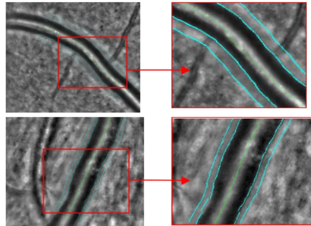
Fig. 8. Images with regularized inner borders and with selected outer borders (images on the left); details (images on the right). Among the three segmentation of the outer border of the walls (one pair of contours in TR1 and two in TR2), the user selects the contours

he wants to analyze on each side of the central reflection (Fig. 8). This approach enables us to deal with the great difficulty of image interpretation (Section IV) while minimizing the expert intervention.

IV.EVALUATION AND DISCUSSION

A database of 15, 17 and 20 images from, respectively, healthy, pathological and vasculitis subjects was gathered, so as to ensure the representativeness of the cases encountered in clinical routine. Images were manually delineated by three physicians, experimented in the field of AO image interpretation. The two first sets of images (healthy, pathological of Type 1), used in [10], is denoted by DB1 in the following, while the set of vasculitis images is denoted by DB2. We evaluate quantitatively the accuracy of a local measure r(s)

obtained automatically (A) by the proposed approach by computing the relative difference in % with the measure derived from a manual segmentation (M): 100 ) ( ) ( ) ( ) ( ) , ( _  _ s r s r s r s _M A M A M r  (6)

The three evaluated measures are the inner radius (denoted IR; b1

and b2 in Eq. 2), the outer radius (denoted OR; b3 and b4 in Eq. 2),

and the wall thickness (denoted WT; b3-b1 and b4-b2 in Eq. 2). For

the images of the database DB2, the wall thickness actually represents the thickness of the perivascular inflammation. These measures are made on every image and on each vessel side. The mean and standard deviation of δr(M,A)(s) are then calculated, and the

results are finally averaged over images and vessels (Tables 1, 2, 3). We chose the manual segmentation of the most experienced physician Phyref as a reference (rM(s) in Eq.6). The same statistics are

computed to evaluate the manual segmentations of the two other physicians with respect to the reference ones, and also the variation between two segmentations of the same physician (inter and intra-physician variability). Since the arterial wall and the perivascular inflammations are very difficult to delineate with a one pixel precision, we also provide the above statics (mean and standard deviation) for a one pixel displacement along the curves. In this case, the numerator in Eq. 6 becomes equal to one. These values are in parentheses in Tables 2 and 3.

The aim of this experimental study is to evaluate the pre-segmentation method proposed in this paper and to compare it with the previous one [10]. The comparison is made on the databases DB1 and DB2 separately. Moreover, the evaluation is performed on the final segmentations, so after application of the CPS active contour model (Section II). The parameters of the CPS model were optimized so as to lead to the most accurate segmentation, on one third of the images of the databases DB1 and DB2, representative of the variability. We found that (ψ=0.02, λ=0.05, φ=100) is the best set of parameters for both kinds of pre-segmentations. The same parameters were used for all the other images.

Table 1 shows the results obtained on DB1 with the previous pre-segmentation method (TRACK+CPS) [9] and the new one (ISO+CPS). For the database DB1, the process of ISO+CPS is fully automatic, as for the method TRACK+CPS, since we only consider one pair of external borders in TR1. In Table 1, we observe that the

ISO+CPS algorithm leads to slightly less accurate measures than TRACK+CPS. The difference is inferior to 1% for the inner and outer radii and inferior to 2% for the wall thickness, which is a very sensitive measurement. The unit displacement along curves indicates that the difference between the two models is inferior to 1 pixel, i.e. 1.6 µm. The p-values (Table 1) calculated to compare the means values of (M,A)(_s)

r

 obtained by TRACK+CPS vs. ISO+CPS, are superior to 5% (Wilcoxon test [14]), so the difference between the two methods on DB1is negligible. Finally, the inter-physician error is about two pixels, so we can conclude that the two models lead to a very good accuracy.

Table 1 Auto vs. Phyref for TRACK+ CPS and ISO+CPS models,

p-values, and inter-physician relative error for the inner radius, the outer radius and the wall thickness, evaluated on DB1, values in %.

TRACK +

CPS ISO + CPS Inter-ph. error p-value Unit displac. along curves IR 4.99 ± 5.58 5.86 ± 8.06 5.18 ± 4.32 42 2.04 ± 0.69 OR 3.71 ± 3.54 4.13 ± 4.39 4.52 ± 3.76 18 1.5 ± 0.46 WT 17.63 ± 15.39 19.02 ± 16.28 21.67 ± 19.59 14 6.16 ± 2.47

Let us now detail the results on the vasculitis database DB2 (Table 2, Table 3). For the database DB2, the process ISO+CPS is not fully automatic, since the method outputs three pairs of external

borders. We keep the pair which is the closest to the reference segmentation. For the three measures, WT, IR and OR, the error on DB2 (Table 2) is higher than on DB1 (Table 1), especially for WT. Indeed the automatic segmentation of the vasculitis walls is particularly difficult, especially in the region of the perivascular inflammation which is very little contrasted. As a consequence, the standard deviation values are close to or even higher than the mean values in Tables 1 and Table 2, showing that the stability of the method is difficult to reach. It is corroborated by the high values of inter-physician (Table 2, Fig. 9) and intra-physician (Table 3, Fig. 9) variabilities, indicating that there is no real consensus among physicians about the accurate location of the outer border of the walls. Table 2 shows that the two automatic methods are equivalent for the inner border, with quite high errors. Indeed the contrast in these images is generally low and the vessel lumen presents often focal narrowing. However the ISO + CPS model is significantly more accurate for the outer borders and wall thickness, and the measures match those of experts.

Table 2 Auto vs. Phyref for TRACK+PCS and ISO+CPS models, and

inter-physician relative error for inner radius, outer radius and perivascular inflammation thickness, evaluated on DB2, values in %.

TRACK + CPS ISO + CPS Inter-ph. error IR 12.87 ± 16.91 (3.16 ± 1.04) 12.78 ± 16.24 (3.16±1.04) 9.39 ± 8.50 ( 2.96±0.95) OR 21.27 ± 17.26 (2.00 ± 0.67) 10.38 ± 9.60 (2.00 ± 0.67) 11.42 ± 11.92 (1.96±0.58) WT 58.89 ± 44.01 (3.91 ± 5.22) 34.60± 38.37 (6.91± 5.22) 46.22±80.18 (7.29±5.70)

Table 3 Intra-physician variability for the inner radius (IR), the outer radius (OR), and the perivascular inflammation thickness (WT),

evaluated on DB2, values in %.

Phys1/ Phys1 Phys2/ Phys2 Phys3/ Phys3 IR 7.32 ± 10.66 (3.11 ± 1.03) 7.18 ± 9.22 (3.06 ± 1.03) 10.32 ± 10.05 (2.96 ± 0.95) OR 8.97 ± 10.85 (1.99 ± 0.63) 8.97 ± 8.28 (2.02 ± 0.67) 8.44 ± 7.63 (1.96 ± 0.58) WT 53.55 ± 2225.25 (16.99 ± 352.20) 35.87 ± 47.57 (15.36 ± 10.17) 40.18 ± 64.07 14.58 ± 11.41

We also computed the root mean square error (Eq. 7) in order to get absolute values expressed in pixel unit. The values are then averaged on vessel borders and images to provide the statistics given in Table 4). These statistics follow the same tendency and confirm the previously analysis.







   N s A M A M r r s r s N RMSE 1 2 ) , ( 1 _{( ) ( )} (7)

Table 4 Statistics on DB1 and DB2 with the quadratic error, in %.

DB1 DB2

TRACK +

CPS ISO + CPS Inter-Ph. error TRACK + CPS ISO + CPS Inter-ph. error IR 2.84±1.64 3.45± 2.55 2.98±1.3 4.94 ± 4.68 4.16±2.45 3.85±1.74 OR 2.99±1.68 3.48± 2.04 3.62±1.89 14.88±11.59 6.32±3.7 7.47 ±5.5 WT 3.45± 1.6 3.91±1.80 4.3± 1.92 14.56±10.77 6.79±3.46 7.99 ±5.46

17.08± 19.42 (IR), 6.97± 5.26 (OR),

25.30± 40.04 (WT) 15.78± 14.01 (IR), 9.64± 7.28 (OR), 25.0± 36.75 (WT)

Fig. 9 Illustration of intra- (left) and inter-physician (right) variability, with relative error values in %.

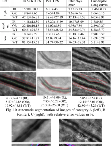
To detail the statistics, the images were classified by the medical experts into three categories according to their quality, considering the contrast of the outer edge of the wall (Table 5): high, medium and low quality (Fig. 10). Of note, this quality evaluation is highly correlated to the inter-physician error for OR. The table confirms the higher quality of the segmentation with the ISO+CPS model than with TRACK+CPS, except for IR in category B. This is due to two images that are particularly difficult to segment (Fig. 11).

Table 5. Statistics on errors with respect to the images category, with relative error values in %.

Cat TRACK+CPS ISO+CPS Inter-phys.

error Unit displac. along curves

hi gh IR _OR 15.78± 10.31 _19.84±7.65 6.1±4.43 _7.65±4.84 7.13±5.23 _7.68±6.56 2.46± 0.29 _1.66±0.15 WT 47.13±36.31 28.42±27.19 32.13±35.53 6.05±2.91 m ed i um IR 14.18±12.80 18.20±15.39 10.47±8.09 3.7±0.55 OR 22.40±10.18 11.02±8.89 9.95±7.59 2.39±0.27 WT 60.81±24.38 33.56±28.92 34.52±40.76 8.28±3.77 lo w IR _OR 10.14±8.29 _32.81±11.27 9.51±7.46 _12.08±9.94 11.18±8.46 _14.16±15.64 2.90±0.52 _1.69±0.28 WT 81.55±15.51 34.74±36.22 56.63±78.31 5.11±2.91 6.77+/-4.31 (IR), 5.57+/-2.88 (OR), 19.92+/-8.81 (WT) 10.61+/-9.09 (IR), 7.85+/-5.22 (OR), 26.30+/-25.60 (WT) 6.85+/-5.54 (IR), 12.44+/-8.01 (OR), 42.80+/-45.29 (WT)

Fig. 10 Automatic segmentation of images of category A (left), B (center), C (right), with relative error values in %.

11.72±10.42 (IR), 8.77±7.52

(OR), 24.21±28.98 (WT) 33.10±27.34 (IR), 14.16±17.21 (OR), 33.55+/-23.88 (WT)

Fig. 11 Accurate (left) and not accurate (right) automatic (magenta) vs. manual segmentation (cyan); relative error values in %. Finally, the method using the TRACK+CPS model is 15 times faster than when using the ISO+CPS model: with an on an Intel® CoreTM _{i7, on DB2 whose images size is about 740-by-740 pixels,}

ISO+CPS model takes on average 1 minute vs. 15 minutes for the TRACK+CPS model. This gain is particularly interesting for the use our software for medical studies in routine practice. Note that the software includes the possibility of local manual correction of the pre-segmentation if the final automatic segmentation is not completely satisfactory.

V. CONCLUSION

The ISO+CPS model presented in this paper is accurate for healthy and pathological images of type 1. It is more adapted to the retinal vasculitis segmentation than the previous TRACK+CPS model and much faster. Moreover, the new model reduces substantially the run time, making it suitable for clinical use. Note that the proposed automatic method is by essence reproducible, while the manual segmentations are not. It is suitable for relative measurements, for instance in follow –up studies, where differences to be assessed can be of the same order of magnitude than the observer variability.

In our future work, we aim at adding an interactive selection of landmarks, thus moving towards a semi-automatic method (instead as a completely automatic one), from which we expect more robustness.

VI. ACKNOWLEGMENTS

This research was supported by the Institut National de la Santé et de la Recherche Médicale (Contrat d’Interface 2011), the Agence Nationale de la Recherche (ANR-09-TECS-009 and ANR-12-TECS-0015-03). We would like also to thank the physicians Edouard Koch and Jonathan Benesty for providing the manual segmentations.

REFERENCES

[1] M.-H. Errera, S. Coisy, C. Fardeau, J.-A. Sahel, S. Kallel, M. Westcott, B. Bodaghi and M. Paques, Retinal vasculitis imaging by adaptive optics,

Ophthalmology, 121(6), pp. 1311, 2014.

[2] M.-H. Errera, J. Benesty, E. Koch, C. Chaumette, J. A. Sahel, B. Bodaghi and M. Paques, Adaptive Optics imaging patterns of retinal vasculitis,

Investigative Ophthalmology & Visual Science, 56(7), pp. 5303, 2015.

[3] J. Liang, D. Williams and D. Miller, Supernormal vision and high-resolution retinal imaging through adaptive optics, Journal of Optical Society America,

A(14), pp. 2884-2892, 1997.

[4] M. Paques, F. Rossant, N. Lermé, C. Miloudi, C. Kulcsar, J.-A. Sahel, L. Mugnier, I. Bloch, K. Loquin and E. Koch, Adaptive Optics Imaging of Retinal Microstructures: Image Processing for Medical Applications, International

Workshop on Computational Intelligence for Multimedia Understanding (IWCIM 2014 ), Paris, France, 2014.

[5] J. Martin, A. Roorda, Direct and non invasive assessment of parafoveal capillary leukocyte velocity. Ophthalmology 112, pp. 2219-2224, 2005. [6] C. Viard, K. Nakashima, B. Lamory, M. Pâques, X. Levecq and N. Château, Imaging microscopic structures in pathological retinas using a flood-illumination adaptive optics retinal camera, Photonics West: Biomedical Optics (BiOS),

7885, pp. 488–509, 2011.

[7] C. Kulcsár, G. Le Besnerais,E. Ödlund, X. Levecq, Robust processing of images sequences produced by an adaptive optics retinal camera,Optical Society

of America, Adaptive Optics: Methods, Analysis and Applications, p. OW3A.3, 2013.

[8] N. Lermé, F. Rossant, I. Bloch, M. Paques and E. Koch, Segmentation of Retinal Arteries in Adaptive Optics Images, International Conference on Pattern

Recognition (ICPR 2014), Stockholm, Sweden, 2014.

[9] N. Lermé, F. Rossant, I. Bloch, M. Paques and E. Koch, Coupled Parallel Snakes For Segmenting Healthy and Pathological Retinal Arteries in Adaptive Optics Images, International Conference on Image Analysis and Recognition

(ICIAR), Vilamoura, Portugal, 2014.

[10] N. Lermé, F. Rossant, I. Bloch, M. Paques, E. Koch and J. Benesty, A Fully Automatic Method For Segmenting Retinal Artery Walls, Adaptive Optics

Images, Pattern Recognition Letters,72, pp. 72-81, 2015.

[11] M. Kass, A. Witkin and D. Terzopoulos, Snakes: Active contour models,

International Journal of Computer Vision, 1(4), pp. 321-331, 1988.

[12] I. Ghorbel, F. Rossant, I. Bloch, M. Paques, Modeling a parallelism constraint in active contours. Application to the segmentation of eye vessels and retinal layers, International Conference on Image Processing (ICIP), pp.

445-44, 2011.

[13] C. Xu and J. Prince, Snakes, shapes and gradient vector flow, IEEE

Transactions on Image Processing, 7(3), pp. 359-369, 1988.

[14] J. D. Gibbons and S. Chakraborti. Nonparametric Statistical Inference, 5th

Ed., Boca Raton, FL: Chapman & Hall/CRC Press, Taylor & Francis Group, 2011.