How Does the Surface Tension Depend on the Surface Area with Coarse-Grained Models?

HAL Id: hal-01790498

https://hal.archives-ouvertes.fr/hal-01790498

Submitted on 8 Jun 2018

HAL is a multi-disciplinary open access archive for the deposit and dissemination of sci-entific research documents, whether they are pub-lished or not. The documents may come from

L’archive ouverte pluridisciplinaire HAL, est destinée au dépôt et à la diffusion de documents scientifiques de niveau recherche, publiés ou non, émanant des établissements d’enseignement et de

To cite this version:

Florent Goujon, Alain Dequidt, Aziz Ghoufi, Patrice Malfreyt. How Does the Surface Tension Depend on the Surface Area with Coarse-Grained Models?. Journal of Chemical Theory and Computation, American Chemical Society, 2018, 14 (5), pp.2644 - 2651. �10.1021/acs.jctc.8b00158�. �hal-01790498�

How does the surface tension depend on the

surface area with coarse-grained models ?

Florent Goujon,

†

Alain Dequidt,

†

Aziz Ghoufi,

‡

and Patrice Malfreyt

⇤,†

†Universit´e Clermont Auvergne, CNRS, SIGMA Clermont, Institut de Chimie de Clermont-Ferrand (ICCF), F-63000 Clermont-Ferrand

‡Institut de Physique de Rennes, Universit´e Rennes 1, 35042 Rennes, France E-mail: Patrice.Malfreyt@uca.fr

Abstract

We propose to investigate the size-e↵ects on the surface tension calculated with coarse-grained (CG) models. We investigate di↵erent vapor (LV) and liquid-liquid (LL) interfaces with the MARTINI forcefield and orignal CG models designed for the dissipative particle dynamics (DPD) and multibody particle dynamics (MDPD) simulations. We also test a realistic CG potential developed for the DPD method to investigate the LV interface of n-pentane. Concerning the MARTINI forcefield, we observe a weak oscillatory e↵ect of the interfacial tension with the surface area for the LV interfaces of n-octane and water. This weak dependence of the surface tension with the box dimension is also observed in the LL interface of n-octane-water (MARTINI, DPD) and in the LV interface of water with the MDPD model.

6 7 8 9 10 11 12 13 14 15 16 17 18 19 20 21 22 23 24 25 26 27 28 29 30 31 32 33 34 35 36 37 38 39 40 41 42 43 44 45 46 47 48 49 50 51 52 53 54 55 56 57

1

Introduction

The coarse-grained (CG) models have been widely applied in molecular simulations of

biomolecules,1 _polymers2–4 _{and surfactants.}5 _{In the CG model, the interactions are}

sim-plified with a CG particle corresponding to many atoms or molecules. These models are designed to model systems on time scales over hundred of nanoseconds that are not acces-sible by standard molecular simulations. Among the various CG force fields, the MARTINI

force field6–12 _{developed by Marrink et al. is by far the most commonly used. This model}

can be implemented in Monte Carlo (MC) and Molecular Dynamics (MD) simulation

meth-ods. Other CG potentials4 _{are used with mesoscopic methods such as dissipative particle}

dynamics (DPD).13–16

There is an increasing need to use these CG models to calculate the interfacial tension of LV and LL interfaces. CG simulations are also important in the industry and in detergency

issues because they can be applied to multi-component mixtures.5 _{A key-property in the}

simulations of these interfacial systems is the interfacial tension. A recent review17 _shows

that some CG force fields present significant deviations of the calculated interfacial tension

from experiments.18 _{The first simulations of the LV interface of water with the MARTINI}

CG model7 _{produced surface tensions of 45 and 30 mN m} 1 _{at 298 K obtained for small}

and big system sizes, respectively. For the electrostatic version of the water MARTINI

model,10 _{the simulated surface tension is found to be 30 mN m} 1 _{while the corresponding}

experimental value19,20 _{is 72 mN m} 1_{. The MARTINI model produces more quantitative}

predictions in the case of the LV interface of alkanes.7 _{The surface tension of water}16 _has

also been calculated from the MDPD method.15 _{In this work, a top-down approach has been}

carried out to develop of the potential parameters.

Even though the calculation of the surface tension from two-phase atomistic simulations of a slab geometry is now under control, it has been at the heart of several debates over

the last 40 years.17,21–38 _{Actually, these slab simulations gave rise to several debates to}

im-portant methodological problems such as the range of the interatomic interactions,31,35,39–41

6 7 8 9 10 11 12 13 14 15 16 17 18 19 20 21 22 23 24 25 26 27 28 29 30 31 32 33 34 35 36 37 38 39 40 41 42 43 44 45 46 47 48 49 50 51 52 53 54 55 56 57

the truncation of the potential,33,39 _{the mechanical and thermodynamic definitions used for}

the calculation of the surface tension33,42–44 _{and the long-range corrections to surface}

ten-sion26–30,32–34 _{and to the configurational energy.}28,32,34,38,44,45 _{An other input parameter that}

may impact the value of the simulated surface tension is the size of the interfacial area. A number of works have reported the dependence of the surface tension of the Lennard-Jones

(LJ) fluid on the surface area.35,46–49_{Figure 1 illustrates this dependence for the LJ fluid by}

showing the ratio of the surface tension to the surface tension ₁ calculated at the largest

surface area.

Nowadays the CG models are extensively used to model large and complex interfacial systems where the surface tension is at the origin of the transport of matter through the interface. As a consequence, it is important to investigate the interface area dependence on surface tension to avoid spurious computational e↵ects. To do so, we propose in a first step to study the impact of the surface area on the interfacial tension calculated by the MARTINI Model. We will investigate the LV interface of water and n-octane. We will complete by the LL alkane-water interface. In the CG MARTINI model, the interactions are calculated by

both the truncated and shifted LJ and Coulombic potentials.18_{In the case of CG interactions}

treated with softer potentials, we will extent the study of the size-e↵ects to a mesoscopic simulation method (dissipative particle dynamics, DPD) by using di↵erent shapes of CG potentials. In a first step, we plan to study the size-e↵ects for generic DPD models for the water LV and oil-water LL interfaces. In these cases, we will use the standard conservative

interactions of the DPD model and its multibody version.15,16,50,51 _{In a second step, we will}

investigate the size-dependence of the interfacial tension of the LV interface of the n-pentane

by using a realistic DPD potential.52

Since the MARTINI and the di↵erent DPD models are the most commonly used for the mesoscale modeling of complex systems, the results concerning the size-dependence of the interfacial tension of coarse-grained interfaces will be very useful for the future simulations in this field. 6 7 8 9 10 11 12 13 14 15 16 17 18 19 20 21 22 23 24 25 26 27 28 29 30 31 32 33 34 35 36 37 38 39 40 41 42 43 44 45 46 47 48 49 50 51 52 53 54 55 56 57

The paper is organized as follows. Section 2 describes briefly the di↵erent potential models, the methods of simulations and the computational details. In Section 3 we discuss the di↵erent finite-size e↵ects of the MARTINI model for di↵erent interfaces. We complete by examining the surface area dependence of the interfacial tension for di↵erent CG DPD models. Section 4 contains our conclusions and recommendations.

2

Model and simulation methodology

2.1

MARTINI model

In the LV interface of the n-octane, the molecule6 _{is described by two beads of type C}

1.

The bonding energy between two beads a and b is calculated by using a harmonic potential

Ubond(rab)

Ubond(rab) =

1

2kbond(rab r0)

2 ₍₁₎

where rab is the distance between beads a and b and r0 the equilibrium distance. The van

der Waals diameter of the CG beads is fixed to 0.47 nm and ✏ is scaled to 75% of the

original value of C1. The values of kbond, r0, and ✏ are listed in Table 1.

The parameters of the polarizable version of the water MARTINI force field10 _{are listed}

in Table 1 et can be found in Ref. 10. In the case of the modeling of the n-octane-water LL interface, the cross-interactions between water (W) and alkane (C1) beads are given in Table 1.

The molecular dynamics (MD) simulations were performed with a modified version of

the DL POLY code.53 _{The changes consist of implementing the shift of the forces from}

rs = 9 ˚A to rc = 12 ˚A. The procedure is described in Ref. 18. The simulations of the LV

interface were carried out in the constant-NVT statistical ensemble with the Nose-Hoover54

algorithm using a thermostat relaxation time of 0.1 ps. For the LL interface, the simulations

were performed in the constant N pNAT statistical ensemble with the thermostat-barostat

6 7 8 9 10 11 12 13 14 15 16 17 18 19 20 21 22 23 24 25 26 27 28 29 30 31 32 33 34 35 36 37 38 39 40 41 42 43 44 45 46 47 48 49 50 51 52 53 54 55 56 57

Nose-Hoover algorithm.55 _{The thermostat and barostat relaxation times were fixed to 0.1}

and 5.0 ps, respectively. The normal component of the pressure tensor pN was maintained

to 0.1 MPa and T = 298 K. The integration timestep was fixed to 10 fs.

The di↵erent bulk liquid phases of octane and water were equilibrated separately during

2⇥ 107 _{steps of simulations (10}7 _{NVT steps followed by 10}7 _{NpT steps). For the LV}

simu-lation, Lz is elongated to form the vapor phase. For LL simulations, the bulk phases of the

two liquids were joined to form the initial configuration. The equilibration phase consisted

of 107 _{steps and the calculation of the average properties was carried out over 10}7 _additional

steps during the acquisition phase. The simulation time of the acquisition phase is then 100 ns.

2.2

DPD method

2.2.1 Generic DPD model

In the DPD method, the total force fi sums three forces: a conservative fijC force, a random

fR

ij force and a dissipative fijD force. The conservative repulsive force fijC is

f_ijC = 8 > < > : aij !C(rij) ˆrij (rij < rc) 0 (rij rc) (2)

where aij is the repulsion energy between beads i and j, rij is the interbead distance

and ˆrij is the corresponding unit vector. rc is the cuto↵ radius. In our DPD and MMC

simulations, the particle mass, the temperature and interaction range were chosen as units

of mass, energy and length. The weight function !C(rij) is defined to 1 rij/rc for rij  rc

and vanishes for rij rc. The expressions of the di↵erent forces can be found in Refs 30,51.

The LL interface of the AB system was simulated by placing an equal number particles of

A and B in the simulation box. The Lz dimension was fixed to 60 in reduced DPD units

corresponding to a reduced number density of 3.0. Lx and Ly were changed from 2.5 to 20.0

in reduced DPD units leading to a variation of a number of particles from 1122 to 72000. The

6 7 8 9 10 11 12 13 14 15 16 17 18 19 20 21 22 23 24 25 26 27 28 29 30 31 32 33 34 35 36 37 38 39 40 41 42 43 44 45 46 47 48 49 50 51 52 53 54 55 56 57

repulsion aAA, aBB and aAB parameters were fixed to 78.0, 78.0 and 105.0, respectively. The

equilibration phase was composed of 106 _{steps and the averages were performed over 5⇥10}6

steps during the production phase. The thermodynamic properties were calculated every 5 steps leading to the calculation of profiles of pressure components and surface tension over

106 _{configurations. The z-dimension corresponds the dimension normal to the interface.}

2.2.2 Generic MMC model

To model a LV interface, the conservative repulsive potential !C(rij) must be modified in

order to consider the local density. In the MDPD approach, the conservative force15,16,50,51

becomes dependent on the local particle density as

f_ijC = A!C(rij)eij + B [ ¯⇢i+ ¯⇢j] !d(rij)eij (3)

where the first term represents an attractive interaction (A < 0) and the second many-body term a repulsive interaction (B > 0). The expressions of the weight functions, the

values of the A and B parameters, the values of rc and rd are given in Ref. 16. Multibody

Monte Carlo (MMC) simulations were carried out using the potential defined by Eq.(4).

UC _{was calculated from the integration of Eq.(3) where u}

i is the energy of particle i and A

corresponds to aij in Eq.(2). UC = N X i uC_i = N X i ✓ ⇡r3 c 30 A X j6=i !⇢(rij, rc) + ⇡r 4 d 30  X j6=i bij!⇢(rij, rd) ⇣ !⇢(rij, rd) + ⇢ 0 i+ ⇢ 0 j ⌘ 2◆ (4)

In Eq.(4) ⇢0_i and ⇢0_j are defined as

6 7 8 9 10 11 12 13 14 15 16 17 18 19 20 21 22 23 24 25 26 27 28 29 30 31 32 33 34 35 36 37 38 39 40 41 42 43 44 45 46 47 48 49 50 51 52 53 54 55 56 57

⇢0_i= X k6=i,k6=j  1 rik rd 2 , ⇢0_j = X k6=j,k6=i  1 rjk rd 2 (5)

If we assume that bij = B we obtain the simplified relation

UC = N X i uC_i = N X i ✓ ⇡r3 c 30 A X j6=i !⇢(rij, R = rc) + ⇡r 4 d 30 B  X j6=i !⇢(rij, R = rd) 2◆ (6)

The systems were equilibrated during 25_{⇥ 10}6 _{steps and the average thermodynamic}

properties were averaged over 25⇥ 106 _{additional steps in the constant-NVT ensemble.}

The simulation boxes were orthorhombic boxes of dimensions LxLyLz. The interfacial area

is defined by A = LxLy where Lx = Ly. The MMC simulations used a simulation cell

constituted by a number of molecules changing from 1000 to 30000 water beads. In this CG model, a bead corresponds to 4 water molecules. This choice implies that the reduced

DPD unit of rc corresponds to 8.52 ˚A. The Lx and Ly dimensions were changed from 36 ˚A

to 111 ˚A. The values of the interaction parameters aij = A and bij = B are 50 and 25,

respectively. These values have been developed in order to reproduce the surface tension16

and the coexisting liquid density of water at 298 K.

2.2.3 Realistic DPD model

For the LV interface of the n-pentane, the pentane is described by one bead. In this

method-ology, the potential !C(rij) was replaced by a tabulated potential which has been developed

by using a new bayesian strategy.52,56 _{The shape of this potential is given for completeness}

later in the paper in Figure 6a. This CG potential has been used in constant-NVT Monte

Carlo simulations with a cuto↵ radius of 20 ˚A at two temperatures 300 K and 400 K. 5

6 7 8 9 10 11 12 13 14 15 16 17 18 19 20 21 22 23 24 25 26 27 28 29 30 31 32 33 34 35 36 37 38 39 40 41 42 43 44 45 46 47 48 49 50 51 52 53 54 55 56 57

⇥105 _{cycles of equilibration were performed to stabilize the interface and additional 2⇥ 10}6

cycles were carried out to average the coexisting densities and surface tensions. When Lx

was changed from 40 ˚A to 100 ˚A the total number of beads increased from 1665 to 104411

and Lz was fixed to 500 ˚A. To study the impact of the change in Lz between 150 and 400

˚

A, Lx and Ly were fixed to 60 ˚A.

3

Results and discussions

As discussed in the introduction of this paper, the truncated Lennard-Jones (LJ) potential is

associated with a strong dependence of the surface tension on the surface area.57 _Depending

on the value of the surface area, the surface tension can vary by ± 20% compared to the

value of surface tension ( ₁) which is defined as the surface tension calculated with the

largest surface area (see Figure 1). It means that along this curve, we can observe significant deviations up to 40% between consecutive values of surface tensions. In the case of LJ

fluids, it is possible to avoid the size-e↵ects dependence17 _{of the surface tension by choosing}

a surface area of 11_{⇥ 11} 2_{. We propose now to investigate the surface area dependence of}

the surface tension of the MARTINI model for di↵erent LV and LL interfaces.

Figure 2a shows the evolution of the surface tension of the LV interface of the n-octane at 300 K. The surface tension is calculated from the integral of the profile along the direction normal to the interface of the di↵erence between the normal and tangential components

of the pressure tensor.58–60 _{For this system, only the repulsion-dispersion interactions are}

modeled by the use of LJ potential. After a small oscillation with an amplitude of 3 mN

m 1 _{that represents a variation of about 15% of the value obtained at the largest interfacial}

area, the surface tension stabilizes around 19.5 mN m 1_{. Any size-e↵ects are detected from}

a surface area of 35_{⇥ 35 ˚}A2_{. The comparison with the corresponding LJ truncated potential}

shows that the surface tension becomes independent of the interfacial area at smaller values

for the MARTINI model (8.5⇥ 8.5 2 _{where = 4.7 ˚A). When electrostatic interactions are}

6 7 8 9 10 11 12 13 14 15 16 17 18 19 20 21 22 23 24 25 26 27 28 29 30 31 32 33 34 35 36 37 38 39 40 41 42 43 44 45 46 47 48 49 50 51 52 53 54 55 56 57

included for the modeling of the LV of water for example (see Figure2b), we observe that

the surface tension is subject to small oscillations of 2 mN m 1_{. The last oscillation is much}

less marked and extends over 40 ˚A. The largest interfacial area simulated here is 100_{⇥ 100 ˚}A

(21_{⇥ 21} 2_{). If we expect a calculation of the surface tension with an uncertainty of 6%, we}

can accept an interfacial area of 60⇥ 60 ˚A2_{. To complete the study with the CG MARTINI}

force field, we represent in Figure 2c the area dependence of the surface tension in the case of the LL interface of octane-water. The amplitude of the oscillations is again around 2

mN m 1 _{which is in the order of magnitude of the statistical fluctuations. This represents}

a change in of 5% compared to ₁. A good convergence of the surface tension with the

interfacial area is obtained from a surface of 70_{⇥ 70 ˚}A2_{. For these three typical interfaces}

using the CG MARTINI model, we can conclude that the interfacial tension is much less sensitive to size-e↵ects by comparison to the truncated LJ potential. This weak dependence of the surface tension calculated with the MARTINI model can be explained by the fact that this force field uses a truncated and shifted potential avoiding any discontinuity at the cuto↵ radius. We have already underlined this point in Ref. 35 where the LJ truncated potential, modified by a spline polynomial, removes the discontinuity in the force and energy equations and reduces significantly the anisotropy of the pressure components.

We now investigate the interfacial tension of an oil-water system where the interactions

are calculated using a conservative CG model 1₂(1 r/rc)2 potential which is continuous

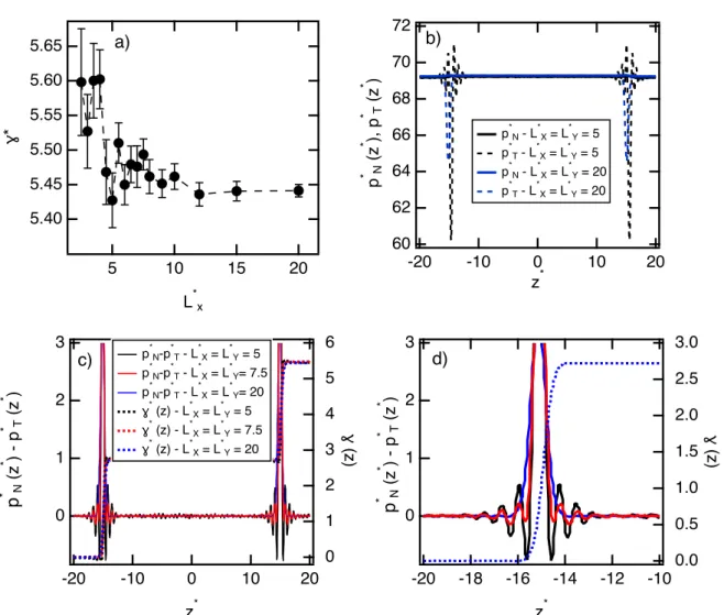
at the cuto↵ radius rc. The simulations were performed using the DPD method. Figure

3a shows the interfacial tension as a function of the interfacial area in reduced DPD units.

For a surface area smaller than 5⇥ 5, the surface tension shows small oscillations of around

2% and the convergence is obtained from L⇤

x = 10. Figure 3b shows the profiles of the

normal and tangential components of the pressure tensor for two interfacial areas. These profiles represent the total pressure components which sum the kinetic and configurational contributions. As expected from the mechanical equilibrium, the normal and tangential components are equal in the two bulk phases with a negative peak of the tangential part in

6 7 8 9 10 11 12 13 14 15 16 17 18 19 20 21 22 23 24 25 26 27 28 29 30 31 32 33 34 35 36 37 38 39 40 41 42 43 44 45 46 47 48 49 50 51 52 53 54 55 56 57

the interfacial region. Part c) of Figure 3 displays the profiles of the di↵erences between the normal and tangential components of the pressure tensor at di↵erent areas. On the right axis of Figure 3, the integral of these di↵erences are also shown for completeness. The profiles

show the same features independently of the surface area : p⇤

N(z⇤) p⇤T(z⇤) is zero in the

bulk liquid phases and present two symmetric peaks at the interfaces. The analysis of ⇤_(z⇤₎

confirms that the two-phase configurations respect the mechanical equilibrium expected for a planar LL interface. Figure 3c also establishes that the di↵erences in the value of the surface tension cannot be attributed to a lack of convergence of the simulations. By focusing

on a specific interface, Figure 3d shows that the profile of p⇤

N(z⇤) p⇤T(z⇤) is subject to small

oscillations at the interface for small interfacial areas. The amplitude of these oscillations decreases with increasing surface areas. For larger surface areas, the profiles do not show any oscillations in the interfacial region whereas their shapes in the bulk phases are much more defined leading to a decrease of the anisotropy of the pressure components.

Figure 4 shows the surface tension of water calculated with a density-dependent CG potential at di↵erent surface areas. The parameters of this potential have been optimized through a top-down a procedure to reproduce the surface tension of water calculated by

using atomistic models.16 _{Simple relationships have been established to link the atomistic}

and mesoscopic length and time scales and operational parameters have been obtained with the MDPD method to reproduce the surface tension, coexisting densities of water at di↵erent temperatures. The degree of coarse-graining was fixed to 4 indicating that a water bead corresponds to 4 water molecules. We propose in Figure 4 to investigate the dependence of

the surface tension of water on interfacial areas changing from 40 ˚A to 120 ˚A. To make a link

with reduced units,16 _{the reduced L}⇤

x should be divided by the cuto↵ rc = 8.52 ˚A indicating

that L⇤

xchanges from 4.7 to 14. This curve shows an oscillatory behavior but with a very weak

dependence of on Lx. No plateau is clearly identifiable on this curve. The maximum and

minimum values of are 73 and 67 mN m 1_{, respectively. These deviations correspond to}

variations of± 4% compared to the value of 70 mN m 1 _{over a large range of L}

xof 80 ˚A. The 6 7 8 9 10 11 12 13 14 15 16 17 18 19 20 21 22 23 24 25 26 27 28 29 30 31 32 33 34 35 36 37 38 39 40 41 42 43 44 45 46 47 48 49 50 51 52 53 54 55 56 57

observed variations are within the statistical fluctuations of the calculation. Let us return to the use of the standard DPD method. We replace the usual conservative potential by a realistic potential model developed from atomistic simulations. The procedure is thoroughly described in Ref. 56 and its application for the calculation of the surface tension of pentane in

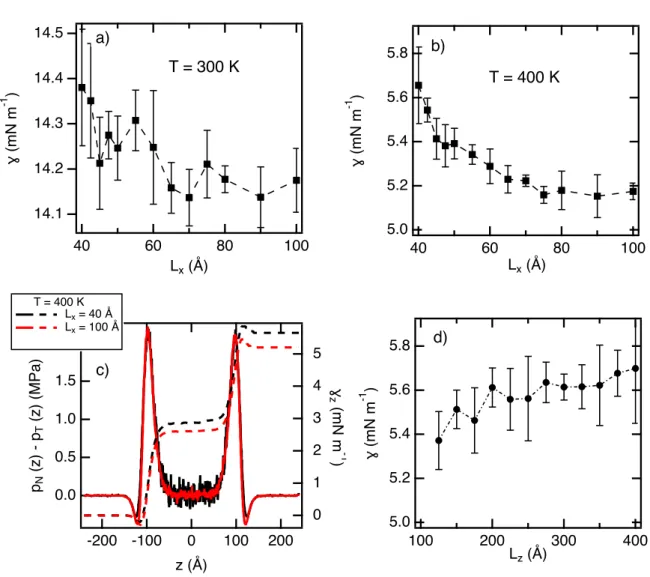
Ref. 52. In a first step, we study the e↵ects of Lx on the surface tension of the n-pentane at

two temperatures. Figure 5a shows that decreases slightly with Lx. Actually, decreases

from 14.4 to 14.1 mN m 1_{with small oscillations leading to a variation of 3% along the range}

of Lx values. As shown in Figure 5b for T = 400K, we observe a monotonic decrease of of

0.45 mN m 1 _{from 40 to 70 ˚A. For larger interfacial areas, we observe a plateau extending}

over 30 ˚A indicating that the surface tension becomes independent of the interfacial area.

The pN(z) pT(z), shown in Figure 5c profiles confirms that the mechanical equilibrium

of the planar LV is verified for the two interfacial areas. Interestingly, for the smallest Lx

value of 40 ˚A, we observe the profile which is much noisier in the bulk phase leads to a

larger surface tension. However, this di↵erence in the surface tension does not come from the contribution of the bulk phase but rather to the interface region on the liquid side as shown in the profile of (z). The dependence of the surface tension on the longitudinal

dimension Lz is shown in Figure 5d. The dependence of on Lz is clearly weak from 125 ˚A

to 225 ˚A with an increase of only 0.2 mN m 1_{. From L}

z = 250 ˚A, we do not observe any

monotonic increase of . The main conclusions we can draw with the di↵erent DPD methods, is that they lead to relatively small dependencies of the surface tension on box dimensions. The di↵erences observed between the di↵erent values are on the order of magnitude of the statistical fluctuations.

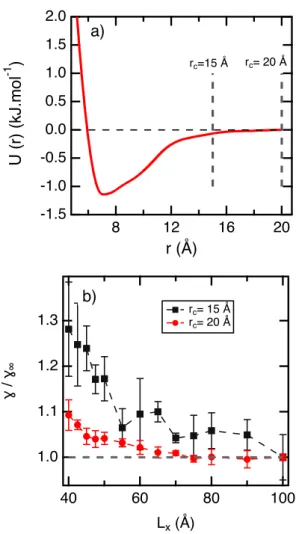
We plan now to investigate the e↵ect of the truncation on the = f (Lx) dependence. We

do so on using a realistic potential of the pentane developed with a cuto↵ rc = 20 ˚A. With

rc = 20 ˚A, the potential decreases smoothly to zero with no discontinuity in the potential

as shown in Figure 6a. We take the route of truncating this potential at a smaller value of

rc = 15 ˚A introducing then a discontinuity at this point. We represent in Figure 6b, the

6 7 8 9 10 11 12 13 14 15 16 17 18 19 20 21 22 23 24 25 26 27 28 29 30 31 32 33 34 35 36 37 38 39 40 41 42 43 44 45 46 47 48 49 50 51 52 53 54 55 56 57

evolution of the ratio of to ₁ at 400 K where ₁ means the surface tension calculated

with the largest box dimension Lx. In both cases, the surface tension decreases with Lx but

the magnitude of the decrease varies from 30% to 10% as rc is changing from 20 ˚A to 15

˚

A. The introduction of the discontinuity in the potential at 15 ˚A increases significantly the

size-e↵ects on the surface tension. This result is in line with observations made with the LJ

potential modified with a cubic spline function.35

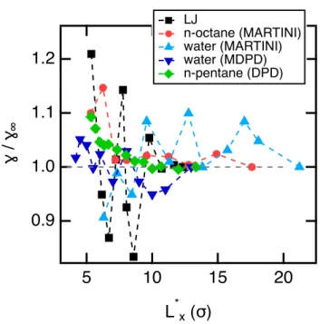
We complete this study by representing on Figure 7 the ratio / ₁ for the LV interface

of di↵erent CG models as a function of the reduced box dimension L⇤

x. The reduced value of

L⇤

xis obtained by dividing the real value by for the LJ and MARTINI models, by rc = 8.52

˚

A for the water MDPD model.16 _{For the pentane DPD model, is defined by the position}

of the well of the CG potential represented in Figure 6a. Interestingly, we observe that the LJ potential give rise to large amplitudes of oscillations with a plateau obtained with three successive oscillations. The water MDPD model is also subject to significant oscillations that

extend over a wide range of L⇤_x. Indeed, these oscillations are not yet stabilized at 22 even if

their amplitude are relatively smaller than those of the LJ fluid. When the MARTINI model is used with only the dispersion-repulsion interactions, e.g in the case of the octane molecule, only one oscillation is observed at 6 . For higher values of the box dimension, there is no more dependence of the surface tension on the surface area. For the mesoscopic simulation methods, the dependence is much less marked. For the water MDPD model, there are small

oscillations but we can consider that reduced interfacial areas of 13⇥13 are acceptable to

avoid any size-e↵ects in the calculation of the surface tension. Finally, in the case of the use realistic DPD model, we observe rather a small decrease of the surface tension with the

interfacial area. We conclude that a reduced interfacial area of 10_{⇥10 is reasonable to avoid}

any dependence of the surface tension.

6 7 8 9 10 11 12 13 14 15 16 17 18 19 20 21 22 23 24 25 26 27 28 29 30 31 32 33 34 35 36 37 38 39 40 41 42 43 44 45 46 47 48 49 50 51 52 53 54 55 56 57

4

Conclusions

Since there is a growing demand in the use of CG models for the calculation of the interfacial tension of complex systems and geometries, it was useful to investigate the dependence of the interfacial tension on the surface area for these models. In the case of atomistic models, it is now well-established that the surface tension of Lennard-Jones fluids exhibits an oscillatory

behavior as function of the surface area. Relatively large surface area of 11_{⇥ 11} 2 _are

required to provide an accurate calculation of the surface tension by using the LJ potential. We have performed a large number of simulations with di↵erent CG models, namely, the MARTINI force field, the standard DPD model and realistic DPD and MDPD models. We have also investigated two types of interfaces : the LV and LL interfaces. Firstly, the size-e↵ects are much less strong with the CG models compared to those observed in atomistic simulations. For the MARTINI model, we observe a weak oscillatory e↵ect with small fluctuations for the LV and LL interfaces. This weak dependence is also observed in the LL interface with the standard DPD model. In the case of the MDPD model for water, the LV surface tension exhibits also a weak oscillatory behavior with small amplitudes. When we use a realistic model for the DPD, we observe that the slight oscillatory behavior observed

at 300 K is replaced by a monotonic decrease of at T= 400 K. We show here that the

truncation impacts the dependence of the surface tension on the surface area as already underlined for atomistic models.

At the end, we give some recommendations to avoid any size-e↵ects of these models by plotting the surface tension as a function of the reduced interfacial area. The di↵erences that appear on the interfacial area dependence with the MARTINI model find their origin in the use of the electrostatic interactions. The surface tension is much less dependent on the surface area with the DPD model even if the water MDPD model is much sensitive to size-e↵ects. 6 7 8 9 10 11 12 13 14 15 16 17 18 19 20 21 22 23 24 25 26 27 28 29 30 31 32 33 34 35 36 37 38 39 40 41 42 43 44 45 46 47 48 49 50 51 52 53 54 55 56 57

References

(1) Arnarez, C.; Uusitalo, J. J.; Masman, M. F.; Ingolfsson, H. I.; de Jong, D. H.; Melo, M. N.; Periole, X.; de Vries, A. H.; Marrink, S. J. Dry Martini, a Coarse-Grained Force Field for Lipid Membrane Simulations with Implicit Solvent. J. Chem. Theory. Comput. 2014, 11, 260–275.

(2) Maurel, G.; Goujon, F.; Schnell, B.; Malfreyt, P. Prediction of Structural and Ther-momechanical Properties of Polymers from Multiscale Simulations. RSC Adv. 2015, 5, 14065–14073.

(3) Maurel, G.; Goujon, F.; Schnell, B.; Malfreyt, P. Multiscale Modeling of the Polymer-Silica Surface Interaction: from Atomistic to Mesoscopic Simulations. J. Phys. Chem. C 2015, 119, 4817–4826.

(4) Espanol, P.; Warren, P. Perspective: Dissipative Particle Dynamics. J. Chem. Phys. 2017, 146, 150901.

(5) Ndao, M.; Goujon, F.; Ghoufi, A.; Malfreyt, P. Coarse–Grained Modeling of the Oil– Water–Surfactant Interface Through the Local Definition of the Pressure Tensor and Interfacial Tension. Theor. Chem. Acc. 2017, 136, 21.

(6) Marrink, S. J.; de Vries, A. H.; Mark, A. E. Coarse Grained Model for Semiquantitative Lipid Simulations. J. Phys. Chem. B 2004, 108, 750–760.

(7) Marrink, S. J.; Risselada, H. J.; Yefimov, S.; Tieleman, D. P.; de Vries, A. H. The MARTINI Force Field: Coarse Grained Model for Biomolecular Simulations. J. Phys. Chem. B 2007, 111, 7812–7824.

(8) Monticelli, L.; Kandasamy, S. K.; Periole, X.; Larson, R. G.; Tieleman, D. P.; Mar-rink, S. J. The MARTINI Coarse-Grained Force Field: Extension to Proteins. J. Chem. Theory Comput. 2008, 4, 819–834. 6 7 8 9 10 11 12 13 14 15 16 17 18 19 20 21 22 23 24 25 26 27 28 29 30 31 32 33 34 35 36 37 38 39 40 41 42 43 44 45 46 47 48 49 50 51 52 53 54 55 56 57

(9) Lopez, C. A.; Rzepiela, A. J.; de Vries, A. H.; Dijkhuizen, L.; H¨unenberger, P. H.; Marrink, S. J. Martini Coarse-Grained Force Field: Extension to Carbohydrates. J. Chem. Theory Comput. 2009, 5, 3195–3210.

(10) Yesylevskyy, S. O.; Sch¨afer, L. V.; Sengupta, D.; Marrink, S. J. Polarizable Water Model for the Coarse-Grained MARTINI Force Field. PLoS Comp. Biol. 2010, 6, 1–17. (11) Sergi, D.; Scocchi, G.; Ortona, A. Coarse-Graining MARTINI Model for

Molecular-Dynamics Simulations of the Wetting Properties of Graphitic Surfaces with Non-Ionic, Long-Chain, and T-Shaped Surfactants. J. Chem. Phys. 2012, 137, 094904.

(12) Marrink, S. J.; Tieleman, D. P. Perspective on the Martini Model. Chem. Soc. Rev. 2013, 42, 6801–6822.

(13) Hoogerbrugge, P. J.; Koelman, J. M. V. A. Simulating Microscopic Hydrodynamic Phenomena with Dissipative Particle Dynamics. Europhys. Lett. 1992, 19, 155–160. (14) Groot, R. D.; Warren, P. B. Dissipative Particle Dynamics: Bridging the Gap Between

Atomistic and Mesoscopic Simulation. J. Chem. Phys. 1997, 107, 4423–4435.

(15) Warren, P. B. Vapor-Liquid Coexistence in Many-Body Dissipative Particle Dynamics. Phys. Rev. E 2003, 68, 066702.

(16) Ghoufi, A.; Malfreyt, P. Mesoscale Modeling of the Water Liquid–Vapor Interface: A Surface Tension Calculation. Phys. Rev. E 2011, 83, 051601.

(17) Ghoufi, A.; Malfreyt, P.; Tildesley, D. J. Computer Modelling of the Surface Tension of the Gas-Liquid and Liquid-Liquid Interface. Chem. Soc. Rev. 2016, 45, 1387–1409. (18) Ndao, M.; Devemy, J.; Ghoufi, A.; Malfreyt, P. Coarse-Graining the Liquid-Liquid Interfaces with the MARTINI Force Field : How is The Interfacial Tension Reproduced ? J. Chem. Theory. Comput. 2015, 11, 3818–3828.

6 7 8 9 10 11 12 13 14 15 16 17 18 19 20 21 22 23 24 25 26 27 28 29 30 31 32 33 34 35 36 37 38 39 40 41 42 43 44 45 46 47 48 49 50 51 52 53 54 55 56 57

(19) Jasper, J. J. The Surface Tension of Pure Liquid Compounds. J. Phys. Chem. Ref. Data 1972, 1, 841–1009.

(20) Vasquez, G.; Alvarez, E.; Navaza, J. M. Surface Tension of Alcohol + Water from 20 to 50 C. J. Chem. Eng. Data 1995, 40, 611–614.

(21) Liu, K. S. Phase Separation of Lennard-Jones Systems: A Film in Equilibrium with Vapor. J. Chem. Phys. 1974, 60, 4226–4230.

(22) Lee, J. K.; Barker, J. A.; Pound, G. M. Surface Structure and Surface Tension: Per-turbation Theory and Monte Carlo Calculation. J. Chem. Phys. 1974, 60, 1976–1980. (23) Chapela, G. A.; Saville, G.; Rowlinson, J. Computer-Simulation of Gas-Liquid Surface.

Discuss. Faraday Soc. 1975, 59, 22–28.

(24) Rao, M.; Levesque, D. Surface-Structure of a Liquid-Film. J. Chem. Phys. 1976, 65, 3233–3236.

(25) Chapela, G. A.; Saville, G.; Thompson, S. M.; Rowlinson, J. S. Computer-Simulation of a Gas-Liquid Surface. 1. J. Chem. Soc. Faraday Trans. II 1977, 73, 1133–1144.

(26) Salomons, E.; Mareschal, M. Atomistic Simulation of Liquid-Vapour

Coexis-tence:Binary Mixtures. J. Phys. Condens. Matter 1991, 3, 9215–9228.

(27) Blokhuis, E. M.; Bedaux, D.; Holcomb, C. D.; Zollweg, J. A. Tail Corrections to the Surface Tension of a Lennard-Jones Liquid-Vapour Interface. Molec. Phys. 1995, 85, 665–669.

(28) Guo, M.; Lu, B. Long Range Corrections to Thermodynamic Properties of Inhomoge-neous Systems with Planar Interfaces. J. Chem. Phys. 1997, 106, 3688–3695.

(29) Goujon, F.; Malfreyt, P.; Boutin, A.; Fuchs, A. H. Direct Monte Carlo Simulations of the Equilibrium Properties of n-Pentane Liquid–Vapor Interface. J. Chem. Phys. 2002, 116, 8106–8117. 6 7 8 9 10 11 12 13 14 15 16 17 18 19 20 21 22 23 24 25 26 27 28 29 30 31 32 33 34 35 36 37 38 39 40 41 42 43 44 45 46 47 48 49 50 51 52 53 54 55 56 57

(30) Goujon, F.; Malfreyt, P.; Tildesley, D. J. Dissipative Particle Dynamics Simulations in the Grand Canonical Ensemble: Applications to Polymer Brushes. ChemPhysChem 2004, 5, 457–464.

(31) Holcomb, C. D.; abd J. A. Zollweg, P. C. A Critical Study of the Simulation of the Liquid-Vapour Interface of a Lennard-Jones Fluid. Mol. Phys. 2006, 78, 437–459. (32) Janeˇcek, J.; Krienke, H.; Schmeer, G. Interfacial Properties of Cyclic Hydrocarbons: A

Monte Carlo Study. J. Phys. Chem. B 2006, 110, 6916–6923.

(33) Ibergay, C.; Ghoufi, A.; Goujon, F.; Ungerer, P.; Boutin, A.; Rousseau, B.; Malfreyt, P. Molecular Simulations of the n-Alkane Liquid-Vapor Interface: Interfacial Properties and Their Long Range Corrections. Phys. Rev. E 2007, 75, 051602.

(34) Shen, V. K.; Mountain, R. D.; Errington, J. R. Comparative Study of the E↵ect of Tail Corrections on Surface Tension Determined by Molecular Simulation. J. Phys. Chem. B 2007, 111, 6198–6207.

(35) Biscay, F.; Ghoufi, A.; Goujon, F.; Lachet, V.; Malfreyt, P. Calculation of the Surface Tension from Monte Carlo Simulations: Does the Model Impact on the Finite-Size E↵ects? J. Chem. Phys. 2009, 130, 184710.

(36) Ferrando, N.; Lachet, V.; P´erez-Pellitero, J.; Mackie, A. D.; Malfreyt, P.; Boutin, A. A Transferable Force Field to Predict Phase Equilibria and Surface Tension of Ethers and Glycol Ethers. J. Phys. Chem. B 2011, 115, 10654–10664.

(37) Werth, S.; Lishchuk, S. V.; Horsch, M.; Hasse, H. The Inflence of the Liquid Slab Thickness on the Planar Vapor-Liquid Interfacial Tension. Physica A 2013, 392, 2359– 2367.

(38) M´ıguez, J. M.; Pi˜neiro, M. M.; Blas, F. J. Influence of the Long-Range Corrections on

6 7 8 9 10 11 12 13 14 15 16 17 18 19 20 21 22 23 24 25 26 27 28 29 30 31 32 33 34 35 36 37 38 39 40 41 42 43 44 45 46 47 48 49 50 51 52 53 54 55 56 57

the Interfacial Properties of Molecular Models using Monte Carlo Simulation. J. Chem. Phys. 2013, 138, 34707–34716.

(39) Trokhymchuk, A.; Alejandre, J. Computer Simulations of Liquid/Vapor Interface in Lennard-Jones Fluids: Some Questions and Answers. J. Chem. Phys. 1999, 111, 8510– 8523.

(40) Lopez-Lemus, J.; Alejandre, J. Thermodynamic and Transport Properties of Simple Fluids using Lattice Sums: Bulk Phases and Liquid-Vapour Interface. Mol. Phys. 2002, 100, 2983–2992.

(41) Grosfils, P.; Lutsko, J. F. Dependence of the Liquid-Vapor Surface Tension on the Range of Interaction: A Test of the Law of Corresponding States. J. Chem. Phys. 2009, 130, 054703.

(42) Gloor, G. J.; Jackson, G.; Blas, F. J.; de Miguel, E. Test-Area Simulation Method for the Direct Determination of the Interfacial Tension of Systems with Continuous or Discontinuous Potentials. J. Chem. Phys. 2005, 123, 134703–134721.

(43) Ghoufi, A.; Malfreyt, P. Entropy and Enthalpy Calculations from Perturbation and Integration Thermodynamics Methods using Molecular Dynamics Simulations: Appli-cations to the Calculation of Hydration and Association Thermodynamic Properties. Mol. Phys. 2006, 104, 2929–2943.

(44) Ghoufi, A.; Goujon, F.; Lachet, V.; Malfreyt, P. Multiple Histogram Reweighting Method for the Surface Tension Calculation. J. Chem. Phys. 2008, 128, 154718. (45) Guo, M.; Peng, B. Y.; Lu, C. Y. On the Long-Range Corrections to Computer

Sim-ulation Results for the Lennard-Jones Vapor-Liquid Interface. Fluid Phase Equilibria 1997, 130, 19–30. 6 7 8 9 10 11 12 13 14 15 16 17 18 19 20 21 22 23 24 25 26 27 28 29 30 31 32 33 34 35 36 37 38 39 40 41 42 43 44 45 46 47 48 49 50 51 52 53 54 55 56 57

(46) Orea, P.; Lopez-Lemus, J.; Alejandre, J. Oscillatory Surface Tension due to Finite-Size E↵ects. J. Chem. Phys. 2005, 123, 114702.

(47) Gonzalez-Melchor, M.; Orea, P.; Lopez-Lemus, J.; Bresme, F.; Alejandre, J. Stress Anisotropy Induced by Periodic Boundary Conditions. J. Chem. Phys. 2005, 122, 094503.

(48) Velazquez, M. E.; Gama-Goicochea, A.; Conzalez-Melchor, M.; Neria, M.; Alejandre, J. Finite-Size E↵ects in Dissipative Particle Dynamics Simulations. J. Chem Phys. 2006, 124, 084104.

(49) Errington, J. R.; Kofke, D. A. Calculation of Surface Tension via Area Sampling. J. Chem. Phys. 2007, 127, 174709.

(50) Ghoufi, A.; Malfreyt, P. Coarse Grained Simulations of the Electrolytes at the Wa-ter/Air Interface from Many Body Dissipative Particle Dynamics. J. Chem. Theory Comput. 2012, 8, 787–791.

(51) Ghoufi, A.; Malfreyt, P. Recent Advances in Many Body Dissipative Particles Dynamics Simulations of Liquid-Vapor Interfaces. Eur. Phys. J. E 2013, 36, 10.

(52) Canchaya, J. G. S.; Dequidt, A.; Goujon, F.; Malfreyt, P. Development of DPD Coarse-Grained Models: from Bulk to Interfacial Properties. J. Chem Phys. 2016, 145, 054107. (53) Todorov, I.; and, W. S. D LPOLY 3: New Dimensions in Molecular Dynamics

Simula-tions via Massive Parallelism. J. Mater. Chem. 2006, 16, 1911–1918.

(54) Nos´e, S. A Molecular Dynamics Method for Simulations In the Canonical Ensemble. Molec. Phys. 1984, 52, 255–268.

(55) Nos´e, S.; Klein, M. Constant Pressure Molecular Dynamics for Molecular Systems. Molec. Phys. 1983, 50, 1055–1076. 6 7 8 9 10 11 12 13 14 15 16 17 18 19 20 21 22 23 24 25 26 27 28 29 30 31 32 33 34 35 36 37 38 39 40 41 42 43 44 45 46 47 48 49 50 51 52 53 54 55 56 57

(56) Dequidt, A.; Canchaya, J. G. S. Bayesian Parametrization of Coarse-Grain Dissipative Dynamics Models. J. Chem Phys. 2015, 143, 084122.

(57) d’Oliveira, H. D.; Davoy, X.; Arche, E.; Malfreyt, P.; Ghoufi, A. Test-Area Surface Tension Calculation of the Graphene-Methane Interface: Fluctuations and Commen-surability. J. Chem. Phys 2017, 146, 214112.

(58) Kirkwood, J. G.; Bu↵, F. P. The Statistical Mechanical Theory of Surface Tension. J. Chem. Phys. 1949, 17, 338–343.

(59) Irving, J. H.; Kirkwood, J. The Statistical Mechanical Theory of Transport Processes .IV. The Equations of Hydrodynamics. J. Chem. Phys. 1950, 18, 817–829.

(60) Rowlinson, J. S.; Widom, B. Molecular Theory of Capillarity; Clarendon Press: Oxford, 1982. 6 7 8 9 10 11 12 13 14 15 16 17 18 19 20 21 22 23 24 25 26 27 28 29 30 31 32 33 34 35 36 37 38 39 40 41 42 43 44 45 46 47 48 49 50 51 52 53 54 55 56 57

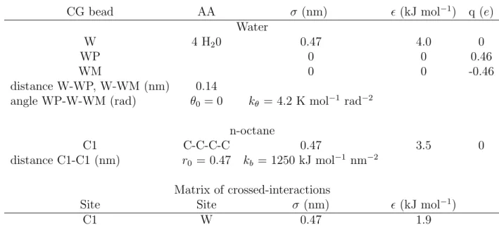
Table 1: Lennard-Jones parameters and electrostatic charges for di↵erent molecules de-scribed through the MARTINI force field.

CG bead AA (nm) ✏ (kJ mol 1_{) q (e)}

Water

W 4 H20 0.47 4.0 0

WP 0 0 0.46

WM 0 0 -0.46

distance W-WP, W-WM (nm) 0.14

angle WP-W-WM (rad) ✓0= 0 k✓ = 4.2 K mol 1 rad 2

n-octane

C1 C-C-C-C 0.47 3.5 0

distance C1-C1 (nm) r0 = 0.47 kb = 1250 kJ mol 1 nm 2

Matrix of crossed-interactions

Site Site (nm) ✏ (kJ mol 1₎

C1 W 0.47 1.9 6 7 8 9 10 11 12 13 14 15 16 17 18 19 20 21 22 23 24 25 26 27 28 29 30 31 32 33 34 35 36 37 38 39 40 41 42 43 44 45 46 47 48 49 50 51 52 53 54 55 56 57

1.3 1.2 1.1 1.0 0.9 0.8 ɣ / ɣ∞ 50 45 40 35 30 25 20 L_x (Å) LJ potential

Figure 1: Ratio of the surface tension to the value of ₁ for di↵erent Lx box dimensions.

1 is calculated with the interfacial area A = LxLy = 46⇥ 46 ˚A2. The data can be found

in Ref. 35 and correspond to the values of methane at T = 120 K. The cuto↵ was fixed to

rc = 2.5 . 6 7 8 9 10 11 12 13 14 15 16 17 18 19 20 21 22 23 24 25 26 27 28 29 30 31 32 33 34 35 36 37 38 39 40 41 42 43 44 45 46 47 48 49 50 51 52 53 54 55 56 57

23 22 21 20 19 18 ɣ (mN m -1 ) 80 70 60 50 40 30 L_x (Å) LV n-octane a) 34 32 30 28 26 ɣ (mN m -1 ) 100 80 60 40 Lx (Å) LV water b) 42 40 38 36 34 ɣ (mN m -1 ) 80 70 60 50 40 30 Lx (Å) LL octane-water c)

Figure 2: Surface tensions of the LV interfaces of the a) n-octane and b) water. c) Surface tension of the LL interface of the n-octane-water system. The surface tensions are calculated

at di↵erent box dimensions Lx defined by

p

A where A is the surface area.

6 7 8 9 10 11 12 13 14 15 16 17 18 19 20 21 22 23 24 25 26 27 28 29 30 31 32 33 34 35 36 37 38 39 40 41 42 43 44 45 46 47 48 49 50 51 52 53 54 55 56 57

5.65 5.60 5.55 5.50 5.45 5.40 ɣ* 20 15 10 5 L*x a) 3 2 1 0 p * (zN * ) - p * (zT * ) -20 -18 -16 -14 -12 -10 z* 3.0 2.5 2.0 1.5 1.0 0.5 0.0 ɣ (z) d) 3 2 1 0 p * (zN * ) - p * (zT * ) -20 -10 0 10 20 z* 6 5 4 3 2 1 0 ɣ (z) p*N-p * T - L * X = L * Y = 5 p*N-p * T - L * X = L * Y= 7.5 p*N-p * T - L * X = L * Y= 20 ɣ* (z) - L*X = L * Y = 5 ɣ* (z) - L*X = L * Y = 7.5 ɣ* (z) - L*X = L * Y = 20 c) 72 70 68 66 64 62 60 p * N (z * ), p * (zT * ) -20 -10 0 10 20 z* p*N - L * X = L * Y = 5 p*T - L * X = L * Y = 5 p*N - L * X = L * Y = 20 p*T - L * X = L * Y = 20 b)

Figure 3: a) Reduced surface tensions of the oil-water LL water calculated using the DPD

method as a function of the reduced L⇤

x dimension. b) Profiles of the normal p⇤N(z⇤) and

tangential p⇤

T(z⇤) reduced pressure components for two interfacial areas. c) Profiles of the

di↵erence between the normal and tangential reduced pressure components with the integral

⇤_(z⇤_{) of this property as a function of z}⇤_{. d) Close-up view of the pressure and surface}

tension profiles at only one interfacial region. All the units are given in reduced DPD units.

6 7 8 9 10 11 12 13 14 15 16 17 18 19 20 21 22 23 24 25 26 27 28 29 30 31 32 33 34 35 36 37 38 39 40 41 42 43 44 45 46 47 48 49 50 51 52 53 54 55 56 57

76 72 68 64 60 ɣ (mN m -1 ) 100 80 60 40 Lx (Å) Water MDPD model

Figure 4: Values of surface tension (mN m 1_{) of water calculated with MDPD simulation as}

a function of the box dimension along the x-dimension.

6 7 8 9 10 11 12 13 14 15 16 17 18 19 20 21 22 23 24 25 26 27 28 29 30 31 32 33 34 35 36 37 38 39 40 41 42 43 44 45 46 47 48 49 50 51 52 53 54 55 56 57

14.5 14.4 14.3 14.2 14.1 ɣ (mN m -1 ) 100 80 60 40 Lx (Å) T = 300 K a) 5.8 5.6 5.4 5.2 5.0 ɣ (mN m -1 ) 100 80 60 40 Lx (Å) T = 400 K b) 2.0 1.5 1.0 0.5 0.0 pN (z) - p T (z) (MPa) -200 -100 0 100 200 z (Å) 5 4 3 2 1 0 ɣ z _{(mN m} -1 ) T = 400 K Lx = 40 Å Lx = 100 Å c) 5.8 5.6 5.4 5.2 5.0 ɣ (mN m -1 ) 400 300 200 100 Lz (Å) d)

Figure 5: Surface tensions of the n-pentane calculated using a realistic tabulated DPD

potential at a) 300 K and b) 400 K. c) Profiles of the di↵erence pN(z) pT(z) at T= 400 K

for two box dimensions. d) Surface tensions calculated at di↵erent longitudinal dimensions

Lz at 400 K. 6 7 8 9 10 11 12 13 14 15 16 17 18 19 20 21 22 23 24 25 26 27 28 29 30 31 32 33 34 35 36 37 38 39 40 41 42 43 44 45 46 47 48 49 50 51 52 53 54 55 56 57

2.0 1.5 1.0 0.5 0.0 -0.5 -1.0 -1.5 U (r) (kJ.mol -1 ) 20 16 12 8 r (Å) rc=15 Å rc= 20 Å a) 1.3 1.2 1.1 1.0 ɣ / ɣ∞ 100 80 60 40 L_x (Å) b) rc= 15 Å rc= 20 Å

Figure 6: a) Coarse-grained realistic tabulated potential between pentane molecules as a function of the distance. The cuto↵ radius is indicated for clarity. b) Ratio of the surface

tension to the value of ₁ calculated for the CG potential truncated at rc = 15 ˚A and

rc = 20 ˚A at 400 K. 6 7 8 9 10 11 12 13 14 15 16 17 18 19 20 21 22 23 24 25 26 27 28 29 30 31 32 33 34 35 36 37 38 39 40 41 42 43 44 45 46 47 48 49 50 51 52 53 54 55 56 57

1.2 1.1 1.0 0.9 ɣ / ɣ∞ 20 15 10 5 L*x (σ) LJ n-octane (MARTINI) water (MARTINI) water (MDPD) n-pentane (DPD)

Figure 7: Ratio of the surface tension to the value ₁ calculated at the largest Lx box

dimensions for the LV interfaces of di↵erent systems and models as indicated in the legend.

The horizontal axis is represented in reduced units of Lx. For the LJ and MARTINI models,

the reduced L⇤

x is equal to Lx/ . For the water MDPD model, the reduced box dimension

is Lx/rc where rc is 8.52 ˚A (see Ref. 16). For the n-pentane DPD model, Lx is divided by

where represents the position of the well of the potential (see Figure 6a).

6 7 8 9 10 11 12 13 14 15 16 17 18 19 20 21 22 23 24 25 26 27 28 29 30 31 32 33 34 35 36 37 38 39 40 41 42 43 44 45 46 47 48 49 50 51 52 53 54 55 56 57

Graphical TOC Entry

Table of Contents use only

How does the surface tension depend on the surface area with coarse-grained models ?

Florent Goujon, Alain Dequidt, Aziz Ghoufi, Patrice Malfreyt

6 7 8 9 10 11 12 13 14 15 16 17 18 19 20 21 22 23 24 25 26 27 28 29 30 31 32 33 34 35 36 37 38 39 40 41 42 43 44 45 46 47 48 49 50 51 52 53 54 55 56 57

1.0

0.9

0.8

ɣ /

50

45

40

35

30

25

20

L

x

(Å)

ACS Paragon Plus Environment

5 6 7 8 9 10 11 12 13 14 15 16 17 18 19 20 21 22 23 24 25 26 27 28 29 30 31 32 33 34 35 36 37 38 39 40 41 42 43 44 45 46 47 48 49 50 51 52 53

20

19

18

ɣ (mN m

80

70

60

50

40

30

L

_x

(Å)

34

32

30

28

26

ɣ (mN m

-1

)

100

80

60

40

L

x

(Å)

LV water

b)

42

40

38

36

34

ɣ (mN m

-1

)

LL octane-water

c)

6 7 8 9 10 11 12 13 14 15 16 17 18 19 20 21 22 23 24 25 26 27 28 29 30 31 32 33 34 35 36 37 38 39 40 41 42 43 44 45 46 47 48 49 50 51 52 53

5.50

5.45

5.40

ɣ*

20

15

10

5

L

*x

3

2

1

0

p

*

(z

N *

) - p

*

(z

T *

)

-20

-18

-16

-14

-12

-10

z

*

3.0

2.5

2.0

1.5

1.0

0.5

0.0

ɣ

(z)

d)

3

2

1

0

p

*

(z

N *

) - p

*

(z

T *

)

-20

-10

0

10

20

z

*

6

5

4

3

2

1

0

ɣ

(z)

p*_N-p*_T - L*_X = L*_Y = 5 p*N-p * T - L * X = L * Y= 7.5 p*N-p*T - L*X = L*Y= 20 ɣ* (z) - L*_X = L*_Y = 5 ɣ* (z) - L*X = L * Y = 7.5 ɣ* (z) - L*X = L * Y = 20

c)

66

64

62

60

p

*

(z

N *

), p

-20

-10

0

10

20

z

* pN - LX = LY = 5 p*T - L*X = L*Y = 5 p*_N - L*_X = L*_Y = 20 p*T - L * X = L * Y = 20

ACS Paragon Plus Environment

6 7 8 9 10 11 12 13 14 15 16 17 18 19 20 21 22 23 24 25 26 27 28 29 30 31 32 33 34 35 36 37 38 39 40 41 42 43 44 45 46 47 48 49 50 51 52 53

68

64

60

ɣ (mN m

100

80

60

40

L

_x

(Å)

Water MDPD model

ACS Paragon Plus Environment

6 7 8 9 10 11 12 13 14 15 16 17 18 19 20 21 22 23 24 25 26 27 28 29 30 31 32 33 34 35 36 37 38 39 40 41 42 43 44 45 46 47 48 49 50 51 52 53

14.5

14.4

14.3

14.2

14.1

!

(mN m

-1

)

100

80

60

40

L

_x

(

_!)

T = 300 K

a)

5.8

5.6

5.4

5.2

5.0

!

(mN m

-1

)

100

80

60

40

L

_x

(

_!)

T = 400 K

b)

2.0

1.5

1.0

0.5

0.0

p

N

(z) - p

T

(z) (MPa)

-200

-100

0

100

200

z (

!)

5

4

3

2

1

0

!

z

_{(mN m}

-1

)

T = 400 K Lx = 40 ! Lx = 100 !

c)

5.8

5.6

5.4

5.2

5.0

!

(mN m

-1

)

400

300

200

100

L

_z

(

_!)

d)

6 7 8 9 10 11 12 13 14 15 16 17 18 19 20 21 22 23 24 25 26 27 28 29 30 31 32 33 34 35 36 37 38 39 40 41 42 43 44 45 46 47 48 49 50 51 52 53

0.0

-0.5

-1.0

-1.5

U (r) (kJ.mol

20

16

12

8

r (Å)

1.3

1.2

1.1

1.0

ɣ /

ɣ

∞

100

80

60

40

L

x

(Å)

b)

rc= 15 Å rc= 20 Å

ACS Paragon Plus Environment

6 7 8 9 10 11 12 13 14 15 16 17 18 19 20 21 22 23 24 25 26 27 28 29 30 31 32 33 34 35 36 37 38 39 40 41 42 43 44 45 46 47 48 49 50 51 52 53

1.0

0.9

ɣ /

ɣ

20

15

10

5

L

*x

(σ)

ACS Paragon Plus Environment

6 7 8 9 10 11 12 13 14 15 16 17 18 19 20 21 22 23 24 25 26 27 28 29 30 31 32 33 34 35 36 37 38 39 40 41 42 43 44 45 46 47 48 49 50 51 52 53